A High-Performance Computing Cluster for Distributed Deep Learning: A Practical Case of Weed Classification Using Convolutional Neural Network Models

Abstract

One of the main concerns in precision agriculture (PA) is the growth of weeds within a crop field. Currently, to prevent the spread of weeds, automatic techniques and computational tools are used to help to identify, classify, and detect the different types of weeds found in agricultural fields. One of the technologies that can help us to process digital information gathered from the agricultural fields is high-performance computing (HPC); this technology has been adopted to carry out projects requiring extra processing and storage in order to execute tasks with a large computational cost. This paper shows the implementation of an HPC cluster (HPCC), in which image processing (IP) and analysis are executed using deep learning (DL) techniques, specifically, convolutional neural networks (CNNs) with the VGG16 and InceptionV3 models, to classify different weed species. The results show the great benefits of using high-performance computing clusters in PA, specifically for classifying images. To apply distributed computing within the HPCC, the Keras and Horovod frameworks were used to train the CNN models, obtaining the best time with the InceptionV3 model with a value of 37 min 55.193 s using six HPCC cores, obtaining an accuracy of 0.65 as a result.

1. Introduction

The classification of weeds is a problem in agriculture, which is why some methods and techniques are carried out manually to identify, classify, and eradicate weeds in crop fields; however, these methods are time-consuming and expensive. For this reason, autonomous methods have been created to manage the growth of weeds in crop fields. Some of these methods consist of using robots [1], UAVs [2], remote sensing [3], and the autonomous identification of weeds to eradicate them at a lower cost, with less effort and time [4].

Currently, algorithms, applications, and methods have been developed that facilitate the identification and classification of different weed species, with the aim of improving the precision of their detection and elimination. DL using CNN is one of the most widely used methods for weed classification. The weed classification process using CNNs is fast and accurate and can be used as a decision-support tool in agriculture [5].

In recent years, researchers and developer organizations have been concerned with the storage and processing of different types of data (video, voice, images, audio, etc.), as storing and processing large amounts of data represent a great challenge. HPC is a way to solve this challenge since its hardware and software capabilities can be added through the interconnection of multiple computers. According to the research and working area, the organizations must choose the technological components that make up the high-performance system (hardware, network infrastructure, storage devices, servers, applications, etc.) that allow data manipulation [6]. Due to the scientific and technological advances in the areas of digital image processing (DIP) and artificial intelligence (AI), it is possible to implement complex algorithms that require high power in computer systems that are accessible to researchers and companies. The architectures or infrastructures that allow exhaustive tasks for the DIP and AI are HPCCs or supercomputers [7]. The evolution of this technology has increased to the point of currently integrating hardware acceleration including the graphics processing unit (GPU) as support in parallel tasks to solve problems with great complexity and computational cost even faster [8]. A supercomputer or HPCC is made up of a set of computers (nodes) interconnected through an ethernet network to share storage, processing, and performance resources, that is, a computer made up of multiple computers. One of the main purposes of supercomputers is to solve computational problems that on a personal computer take too long to solve [9]. HPC and autonomous learning techniques, such as machine learning (ML) and deep learning (DL), are some of the technologies that have been adopted to solve the problems of the storage and processing of data obtained from crop fields [10].

Analysis and image classification in AI are some of the topics with great importance within the scientific community since due to the methods and algorithms used, it is possible to obtain important data from a certain selection of images that can help us generate knowledge of any kind [11]. Artificial neural networks (ANNs) are computational models composed of multiple processing layers that serve to perform automatic learning based on the use of structures and large amounts of data; convolutional neural networks (CNNs) are a type of ANN that precisely help us to solve image processing problems that represent problems we encounter in modern life [12]. The adaptation of AI within PA has been benefiting farmers for years in its ability to solve some of the frequent problems that occur in crop fields, such as pest and infestation control, grass control, administration of water resources, and application of pesticides, among other activities that have been carried out individually and that can now be automated [13]. One of the most applied new methods or technologies in this area is ANNs. The main benefit of neural networks (NNs) is that they can predict, classify, and forecast some behavior patterns in agricultural fields, based on the data provided to them in training the NN [14].

Specialized devices such as graphics cards allow one to run CNN models or architectures. An NVIDIA graphics card is one such device used to implement HPCC and machine learning models to take advantage of the parallel processing and performance driven by GPU nodes [15].

HPCCs allow data to be stored on a large scale, and with the help of some free software platforms, statistical analysis or learning can be conducted with the data obtained, in this case, images. Due to the above, the use of technological tools such as CUDA, Open MPI, and Python has been proposed to implement an HPCC to enable the performance of the aforementioned tasks and make the processing and analysis of crop field images more efficient.

Therefore, the decision was made to combine HPC technology with CNNs to classify weed species in an HPCC. Although there are already implemented HPCC architectures, such as Fugaku, SUMMIT, SIERRA, Sunway, Perlmutter, and others, which are within the top of the TOP500 list [16], as well as architectures existing in Mexico, including the LEO ATROX from the Data Analysis and Supercomputing Center (CADS) of the University of Guadalajara [17], the National Supercomputing Laboratory of Southeast Mexico (LNS) [18], the Laboratory National High-Performance Computing (LANCAD) [19], and the Galileo of the Autonomous University of Zacatecas (UAZ) [20], none of these were used.

For this article, an HPCC was implemented with mid-range desktop computers, which, due to their characteristics, were useful for the distributed processing of CNNs. This decision was made as access to current HPC architectures has a high cost, requiring bureaucratic procedures to request the services they offer, which sometimes take a long response time [21].

This article aims to demonstrate that HPC technology can be accessed using idle or convenient computers to unify their processing and storage capabilities and use them for AI projects. For the validation of this HPCC, a weed classification process was carried out through the use of DIP and distributed DL; specifically, a CNN was applied to crop images. In addition, the processing time between a workstation and the proposed HPCC was also compared. For this, two pretrained CNN models were used, which were InceptionV3 and VGG16. We used the “DeepWeeds” dataset [22] to observe the behavior of the processing speed and the accuracy of the weed classification.

2. Materials and Methods

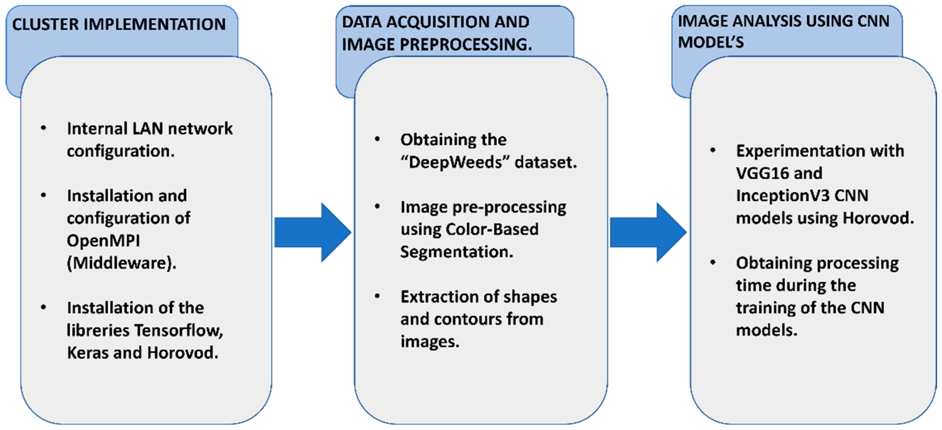
In this article, a methodology is presented that serves to implement an HPCC made up mainly of computers that were available in a university computer lab. The results of the test that was carried out on this HPCC were compared with those obtained from the same experiment on a workstation.

Figure 1 shows the proposed methodology for the implementation of our HPCC that was tested, using distributed deep learning and relying on the Python frameworks for deep learning: TensorFlow [23], Keras [24], and Horovod [25].

2.1. HPCC Design

Distributed computing refers to the use of multiple computers or processors to work together on a task. In a distributed computing system, each computer or processor in the system has its own memory and computational resources, and they communicate and coordinate with each other to perform a task.

One of the main advantages of distributed computing is that it can provide greater computing power and scalability than a single computer. By breaking a task into smaller pieces and distributing them across multiple processors, a distributed computing system can perform the task faster than a single computer. Additionally, distributed computing can provide fault tolerance and resilience as the system can continue to function even if one or more processors fail. However, it requires careful design and management to ensure that it operates efficiently and securely [26].

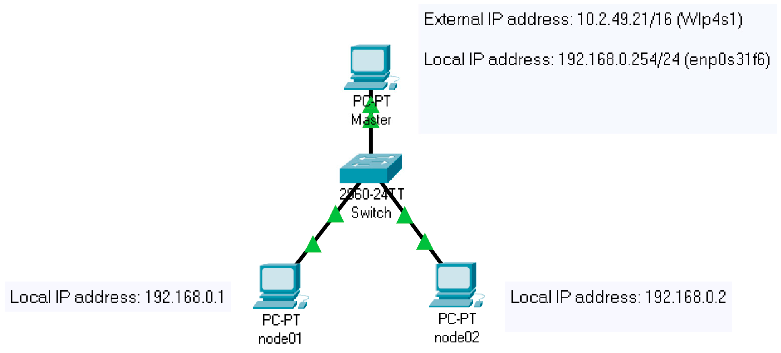
An HPCC is a type of distributed computing system that consists of multiple computers or multiple nodes connected through a local area network (LAN), commonly with ethernet technology. There are several network interconnection options for clusters such as ethernet, FastEthernet, and GigabitEthernet (some examples of interconnected technologies used in HPC include InfiniBand and Myrinet) [27]. An ethernet network can be interconnected by devices that enable Gbit ethernet bandwidth speeds. For this article, the master node, for example, had two network interface cards (NICs), one wireless (wlp4s1) and one wired (enp0s31f6). The other three computing nodes also had two cards, but it was only essential to use the wired one (enp0s31f6). All the computers were connected to a CISCO 2960 switch, which allowed connecting the interfaces with Gbit ethernet width (high-speed ethernet). Figure 2 shows the network diagram and the IP addressing table of the proposed HPCC infrastructure.

The master node was the only computer that had two interfaces connected; one went to the local network and the other to the external network, in this case, the wireless network of the building, where the HPCC was positioned.

It is important to note that the IP addressing of the local network belonged to a type of private addressing; that is, the IP addresses used in the devices were unique and exclusive to that network.

The graphics cards installed in each of the PCs, as well as the CUDA library, were configured for practical and experimental purposes, with the purpose of adding extra processing in this HPCC. Up to this part, we had the design of the network that represented the HPCC, which, over time, could continue to increase the number of connected computers. As the size of the cluster increases, so does the complexity of the system, which can make it more difficult to manage and keep it running. This is why it is important to scale an HPCC considering the budget, installation area, and computing problems that it will solve. Distributed computing in weed classification using CNNs can be a challenging task that requires expertise in multiple areas, not only in the computing sciences.

Designing and building an HPCC can be expensive, and the costs can quickly escalate if the hardware or software components are not selected carefully. Therefore, cost effectiveness must be considered during the design process.

2.2. HPCC Configuration

Normally, the master node of an HPCC infrastructure is the one that contains the servers of the network services since it is the device in charge of the administration of the local network, users, and applications to be executed; that is why, as observed in

Table 1. The proposed HPCC IP addressing and service assignment table.

Device	Interface	IP Address	Network Services
Master	Wlp4s1 enp0s31f6	10.2.49.21/16 192.168.0.254/24	NFS Server, DNS, DHCP, SSH server, CUDA, OpenMPI, Python, OpenCV, Tensorflow, Keras, and Horovod
node01	enp0s31f6	192.168.0.1/24	NFS client, SSH server, CUDA 11.7, and OpenMPI
node02	enp0s31f6	192.168.0.2/24	NFS client, SSH server, CUDA 11.7, and OpenMPI

, the computing nodes have the client services and the master node the servers.

The services in charge of managing the network resources allow communication at the transport layer level between the HPCC nodes. Usually, the services that the infrastructure must have include a domain name system (DNS), a dynamic host control protocol (DHCP), a network file system (NFS), a secure shell (SSH), the web, and a firewall [21]. The configuration of the network services in an HPCC is a critical process that must be carried out in the proper order to guarantee the correct operation of the system. The configuration should start with configuring the physical network and continue with configuring the IP addresses, DNS and DHCP, NFS, SSH, and the firewall.

Another of the fundamental parts that exists within HPC is the middleware, which is essentially the supplementary software that connects two or more software together [28]. With the help of middleware, it is possible to integrate applications with parallel programming environments.

In addition to the previous services, applications such as OpenMPI and MPICH were installed, which were the applications that allowed tasks to be executed in parallel within the HPCC; these were mainly in charge of distributing the processes in each of the nodes and used programming languages such as Python, Java, Fortran, C, C++, etc. [27].

OpenMPI provides a set of libraries and tools that allow developers to write parallel programs using MPI. These programs can be used to solve a wide range of scientific and engineering problems, including simulations, data analysis, and ML.

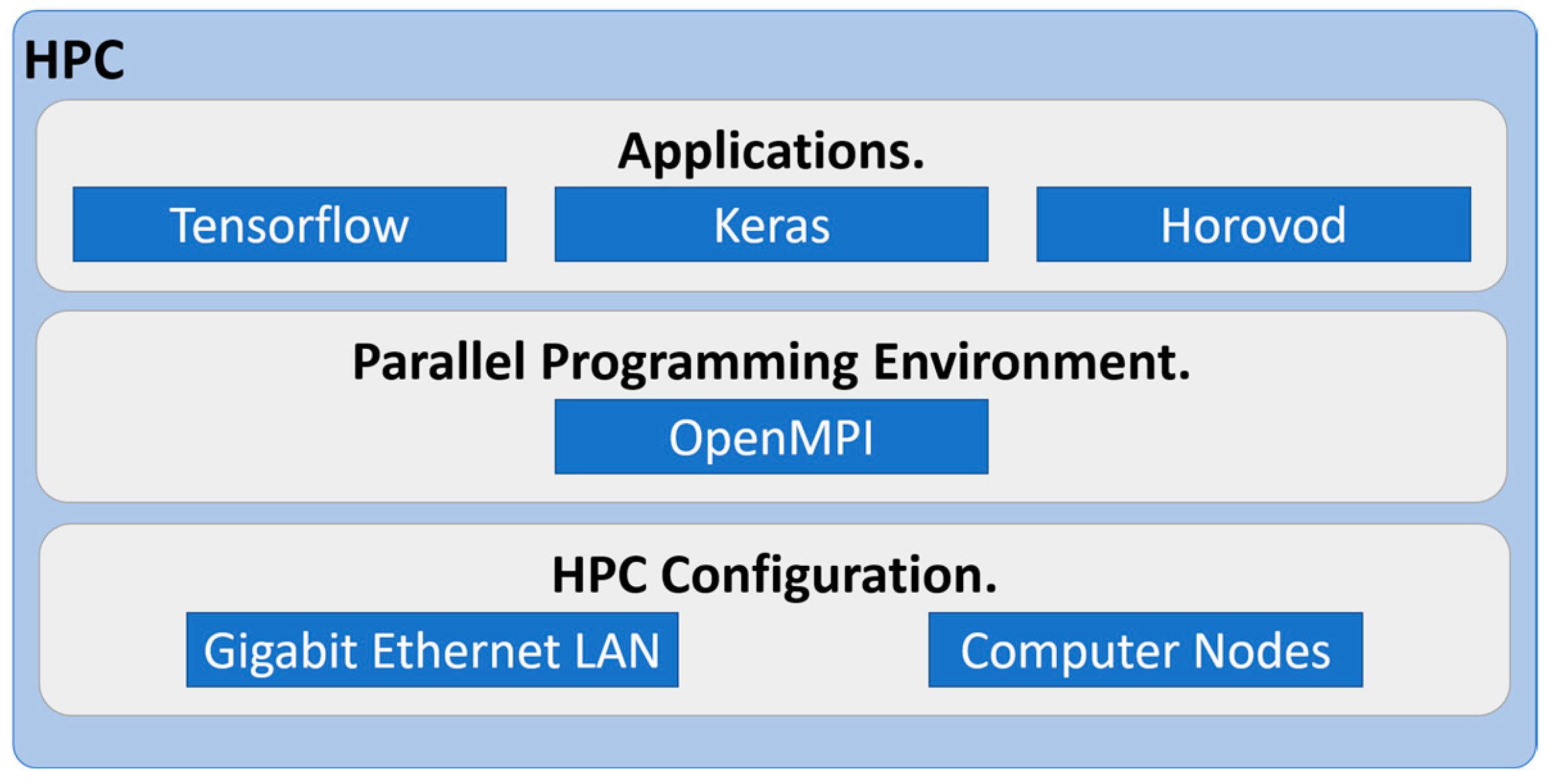
The software for the HPCC should be optimized for distributed computing and ML. Popular DL frameworks such as TensorFlow, PyTorch, and Caffe should be used to implement the CNN models. The software should be designed to take advantage of the distributed architecture of the HPC by using techniques such as data parallelism and model parallelism. In this case, Horovod was used to implement the CNN models to classify images of weeds using this HPCC and distributed DL. The combination of HPC and DL for weed classification was a good option if we wanted to obtain excellent results in a shorter time.

Figure 3 represents the minimum logical configuration of the proposed HPCC.

2.3. HPCC Implementation

Usually, for the construction of an HPCC, devices with server or workstation characteristics are used. As previously mentioned, the choice of devices depends on the budget and scalability; however, on this occasion, since there was no high budget, we opted for hardware or devices with the characteristics shown in

Table 2. Characteristics of the computers used to implement the CPU cluster.

Node	Node RAM	Processor	HDD	Graphic Card	No. CPUs	CUDA Cores	GC RAM
Master node	16	Intel i7-7700K	240 GB	GTX 1050ti	4	768	4 GB
Node01	16	Intel i7-7700K	500 GB	GTX 1050ti	4	768	4 GB
Node02	16	Intel i7-7700K	500 GB	GTX 1050ti	4	768	4 GB
Workstation	32	AMD Ryzen 9500X	1 TB	RTX 3070	12	5888	8 GB

. For greater ease of adaptability at the time of configuration, it is recommended that all the equipment be similar or the same in model, processing, and storage.

An HPCC can be made up of different computer or device architectures. For this implementation, it is important to mention that not all the computers or nodes were of the same brand model (they were assembled), which is a typical and common situation in most cases where one wants to assemble or configure an HPCC with equipment or devices that are no longer used or are collected from different areas of a research center, university, or company.

Table 2 describes the hardware characteristics of each of the computers used for the implementation of this HPCC.

The Ubuntu Server 18.04 Operating System was installed on each of the computers, which allowed users to interact with the tools of the HPCC. In order for the infrastructure to function correctly, the aforementioned network services were installed and configured to be able to manage both the users and the applications necessary for user interaction with the HPCC; it is also important to mention that the applications must co-exist or must be compatible for the processing to be carried out correctly. In the event that any of the applications are not compatible or have missing dependencies, the executions or processes that need to be carried out in a distributed or parallel manner cannot be run within an HPCC.

2.4. Weed Classification

This section describes the process that was carried out for weed classification using the HPCC configured in the previous section using the distributed DL.

DL in precision agriculture in recent years has had numerous applications; crop field monitoring and management, crop field identification and prediction, yield prediction, disease and pest detection, and development of autonomous farming equipment stand out. The above provides farmers or the agricultural industry with efficient methods to maximize the growth of the products and the good administration of the crop fields [29]. In the case of weed classification, methods that combine image processing and deep learning are used to optimize a plant control strategy for infestations that may thwart the growth of the desired plants in crop fields.

A CNN can be used for weed classification by training the model on a dataset of images of different types or classes. The CNN can learn to recognize patterns and features in the images that distinguish one type or class from another [12]. The CNNs achieve a recognition accuracy in images depending on the architecture or model of the neural network, that is, the number of layers and the depth that it possesses [30].

2.4.1. Data Acquisition CNN

In PA, obtaining the relevant information, such as the vegetation indices, soil administration, and weed classification, among others, from crop fields is one of the main objectives.

That is why a weed classification exercise was carried out with DL using a dataset as input to our proposal and then obtaining the processing time and the accuracy of the results.

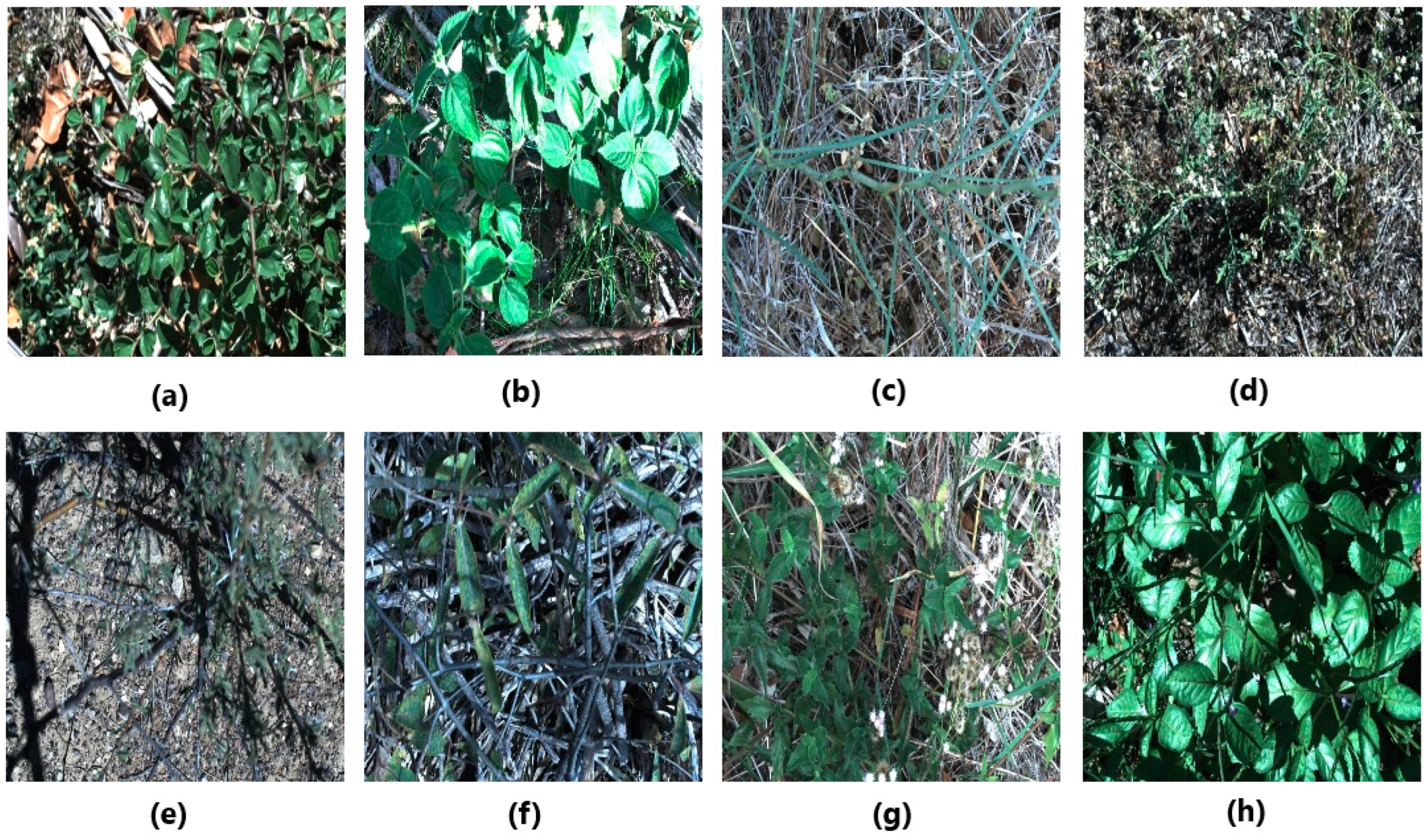
The dataset was composed of images of weed species called “DeepWeeds” [22], which contained 17,509 images of different plant species obtained from different environments in northern Australia, as shown in Figure 4. It was created in order to provide an instrument that would allow the classifying of a variety of weed species through a robotic system. The dataset can be obtained through the following link: https://github.com/AlexOlsen/DeepWeeds (accessed on 3 February 2023).

The collection of the images in this dataset was conducted through a platform that consists of the use of a Raspberry Pi, a high-resolution camera (1920 × 1200 px) FLIR Blackfly 23S6C, Fujinon CF25HA-1 computer vision lenses, a SkyTraq GPS receiver Venus638FLPx, a VTGPSIA-3 GPS antenna, and an Arduino Uno board [22].

2.4.2. Data Preprocessing

For this work, the dataset underwent preprocessing, consisting of applying the color-based segmentation method to each of the images contained in the dataset in order to extract the shape of the undergrowth so the CNN models further classified each of the weed species.

The conversion from an RGB to an HSV color space model is defined by Equations (1)–(3) [31]:

$$H=\left\{\begin{array}{c}0, si Max=Min\\ \left(60°\times \frac{G-B}{Max-Min}+360°\right)\times mod 360°, si Max=R\\ 60 °\times \frac{B-R}{Max-Min}+120°, si Max=G\\ 60 °\times \frac{R-G}{Max-Min}+240°, si Max=B\end{array}\right.$$

(1)

$$S=\left\{\begin{array}{c}0, si Max=0\\ \frac{Max-Min}{Max}, any other value\end{array}\right.$$

(2)

$$V=Max$$

(3)

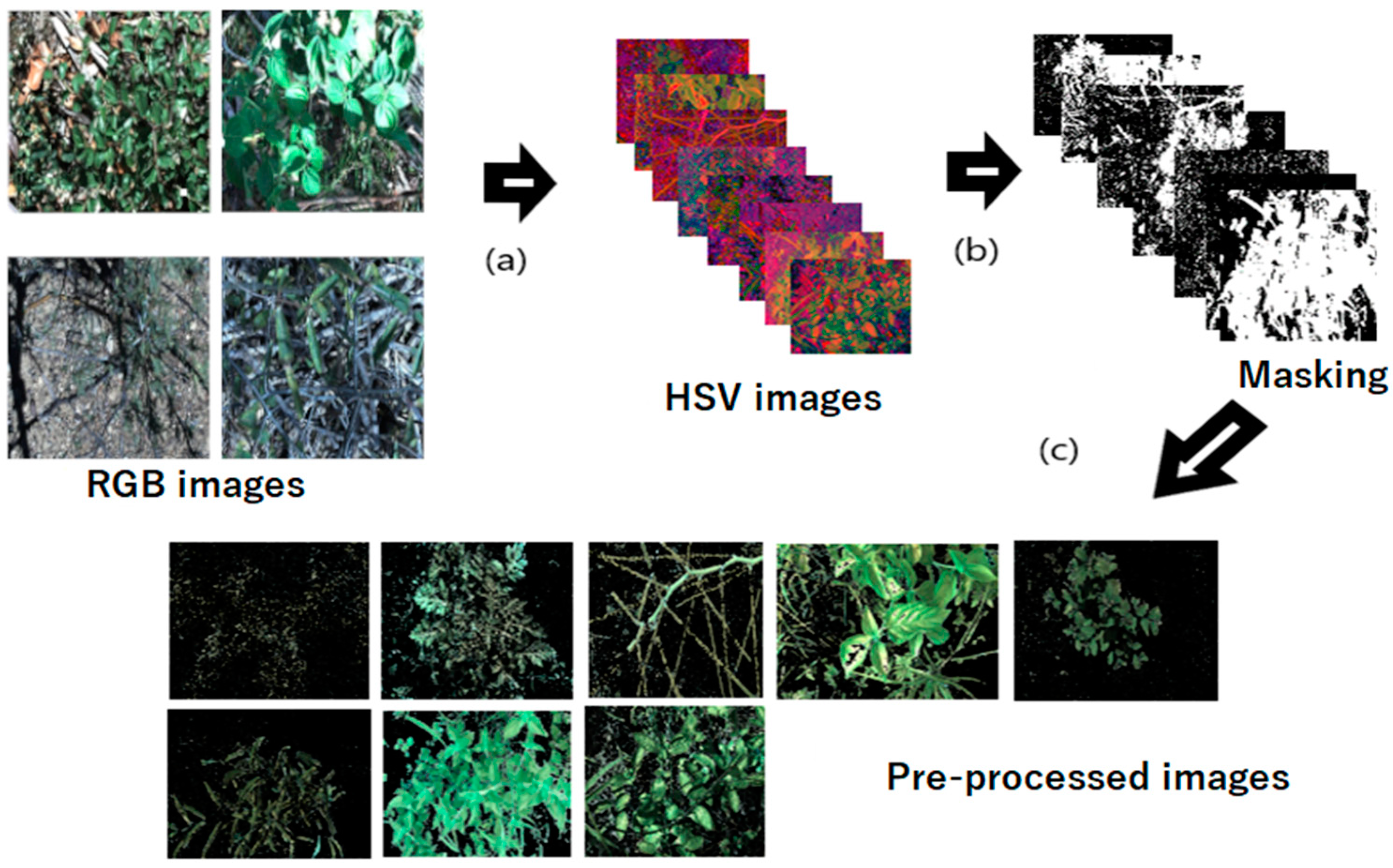
where Max is the maximum value of the RGB color model components, Min is the minimum value of those same components, and mod is a modular operation with 360 degrees. Figure 5 represents the process of the color conversion and masking of the preprocessed images.

The procedure to carry out the segmentation of the dataset images consisted of (a) converting the red–green–blue (RGB) color images to hue saturation value (HSV); once this was complete, the masking was performed (b), and finally, the shapes of each of the weeds (c) were obtained. It is important to mention that all the preprocessing of the images was performed using the OpenCV library; so, only the functions corresponding to each process were applied, and we considered a vector of features with green hues defined between 50 and 150 [32]. The effectiveness of the color-based segmentation for weed detection depends on the color properties of the weed and the background, as well as the lighting conditions and the camera settings used to capture the image. In some cases, other features such as texture, shape, or size may need to be used in combination with color-based segmentation for more accurate weed detection.

2.4.3. Training and Evaluation of the CNN for Weed Classification

Once the preprocessing was complete, two CNN models were used to train and classify the different classes of weed species found in the “DeepWeeds” dataset, Inception V3 and VGG16.

The CNN InceptionV3 architecture is one of the widely used image recognition models, which was shown to achieve greater than 78.1% accuracy on the ImageNet dataset. The model is made up of symmetric and asymmetric building blocks including convolutions, average-pooling, max-pooling, concatenations, pullbacks, fully connected layers, batch normalization, and trigger inputs, and the losses are calculated via a Softmax function [33]. The following image shows an example of the CNN InceptionV3 architecture.

The architecture of the CNN VGG16 is formed by 13 convolutional layers, two fully connected layers, and a Softmax classifier; this network was created in order to use only 3 × 3 convolutional layers stacked one on top of the other. It is one of the CNNs that offers the ability to extract features from the images; so, it is widely used when large amounts of these need to be processed [34].

2.4.4. Distributed DL Using Horovod

Thus far, we have explained how the HPCC was used, the preprocessing of the images, and the models of convolutional neural networks that were used. Now, we briefly explain how the distributed DL was conducted, for which the Horovod framework was used. We decided to use the Horovod framework as, in terms of acceleration, it allows for reducing processing times when processing large amounts of data in a distributed manner [35].

The Horovod allows training CNN models in distributed systems, using OpenMPI configurations and the NVIDIA Collective Communications Library (NCCL) to support communications between GPUs [36]. To adapt the Horovod framework with Keras, it was necessary to make some modifications in the scripts so that the application ran correctly [37]. The actions that the Horovod performed for the distributed training of the parallel data were conducted in the following order:

• Multiple copies of the script were created, and each copy was executed on each of the processing nodes, calculating the gradients of the models that ran through them.
• The number of gradients of the copies created was averaged.
• The model was updated.

The above steps were repeated.

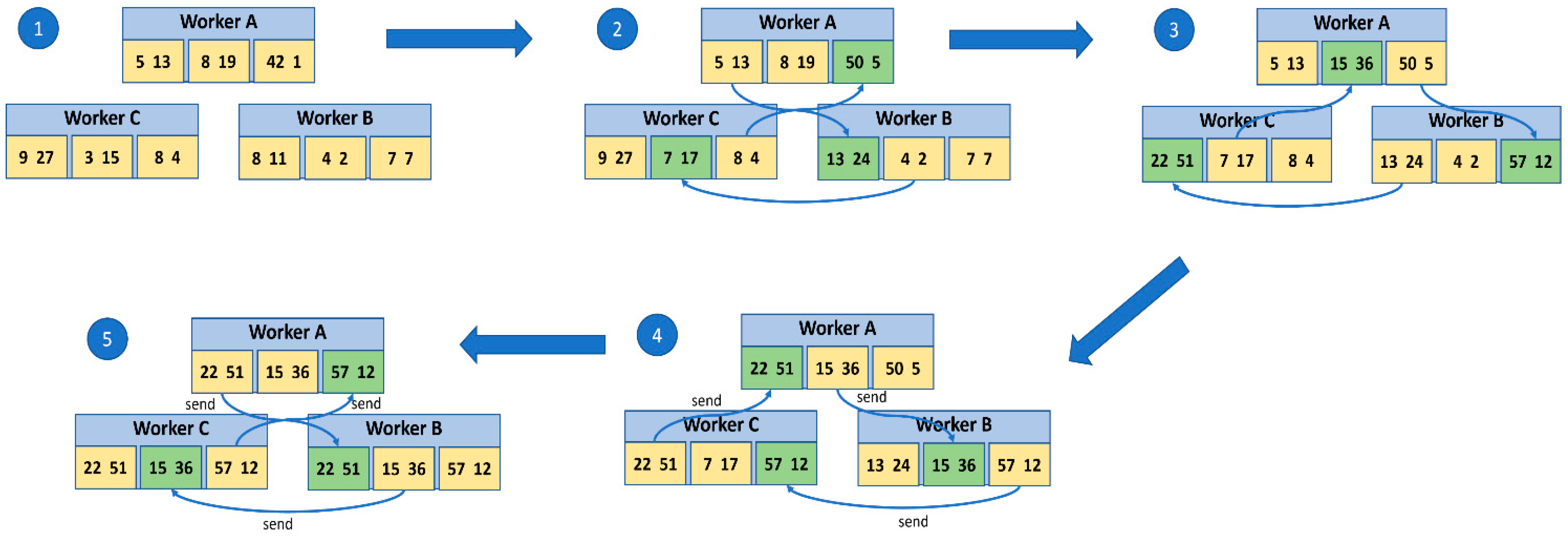
As mentioned above, OpenMPI was used for the experiment, which has the AllReduce communication primitive, which, within Horovod, is an operation that is based on the Ring Allreduce algorithm, where all workers communicate with each other in a network topology ring. Each worker calculates their own slopes and sends them to their neighbor in the ring. When a worker receives gradients from their neighbor, it adds them to its own gradients and sends the result to the next neighbor in the ring. This process continues until all workers have received the merged gradients.

The Horovod Allreduce uses a combination of MPI and NCCL to optimize communication and computation for training DL models. By leveraging these libraries, the Horovod Allreduce can efficiently scale up to thousands of CPUs or GPUs, reducing the training times and improving performance. In this algorithm, each N nodes communicate with two of their peers 2 × (N − 1) times. During communication, a node sends and receives some buffered data frames. In the first iteration (N − 1), it receives values that are added to the node’s buffer values. In the second iteration, the received values maintained by the node buffer are replaced [38]. Figure 6 shows the process in which the gradients are calculated using the Allreduce algorithm.

For the “DeepWeeds” dataset experiment, 400 images of each weed species class were considered, giving a total of 3200 images. For the distribution of the data, 70% of the images (2240) were considered for the training set with the rest 30% (960) for the testing set. Being a supervised method, the weed species classes were previously labeled in folders.

One of the important settings for CNN models is the batch size, which is the number of samples taken for each gradient update. For the tests, a batch size of 64 was established in each CNN model; that is, each gradient update was made from 64 data points.

Another configuration to train the model is the epochs, which represent the iterations that are performed on the input data and the output data using the batch size value as the increment factor. For the implemented models, the following value was considered: epochs = int(math.ceil(100.0/hvd.size())), where the value of the epochs was equal to the value of 100 divided by the total number of processes in the HPCC defined by the argument –np of the command horovodrun [36]. The function math.ceil() indicates that if the value was not an integer, that is, if a value of 12.3 were obtained, the correct value would be 13.

A procedure called stochastic gradient descent (SGD) [39] is widely used in most projects related to ML and large-scale learning. This method consists of displaying an input vector for some examples, calculating the outputs and errors, calculating the average gradient for those examples, and adjusting the weights. The process is repeated for many small training set instance processes until the average of the average function stops decreasing. It is called stochastic because each small part of the set of examples provides a noise estimate of the average of the gradient over all the examples [6]. The learning range is nothing more than a value between 0.0 and 1.0 that controls the speed with which a CNN model adapts to the problem or classification.

There are linear functions used in neural networks including ReLU (rectified linear unit), which is activated by any value greater than 0, and its mathematical representation is $f\left(x\right)=max\left(0, x\right)$ [40].

The activation function used in the code implemented for the CNN Horovod library for the experiment was that of ReLU since it is one of those commonly used to connect the convolutional layers.

Another important function used within ML for multiple classifications is Softmax, also used in fully connected layers. Softmax is a normalized exponential function that represents the categorical distributions and compresses arbitrary vector values within the range [0, 1].

Finally, the Keras library has several pretrained CNN models that can be implemented for classification and feature extraction [41]. Some of the models available are

• Xception.
• VGG16/19.
• ResNet/ResNetV2/50/101/152.
• InceptionV3.
• InceptionResNetV2.
• MobileNet/MobilNetV2.
• DenseNet/121/169/201.
• NASNet/Mobile/Large.

How CNN models work sometimes depends on the version of Keras installed. In higher versions of Keras 2.2.0, the image size must be the one defined by default for each of the models or at least 150 × 150 pixels. Since the size of the images used for this project was 100 × 100 pixels, version 2.4.0 had to be installed.

2.5. Performance Metric on the HPCC and the Workstation

To evaluate an HPCC, different metrics are used that allow measuring the performance and efficiency with which it solves problems that require high processing power. Some of the metrics are floating point operations per second (FLOPS), processing time or speedup, memory bandwidth, energy efficiency, scalability, and network latency, among others [42]. For this research, only FLOPS were considered.

The FLOPS measurement is a way of evaluating the processing capability of a computer system in relation to performing floating point operations. For example, a computer that can perform 100 teraflops (100 trillion floating-point operations per second) is capable of processing a large number of mathematical calculations in a relatively short period of time, which can be important for applications that require large amounts of data. It measures the number of intensive computations in terms of processing.

To calculate the FLOPS of a computer, we first need to know the specification of the processor and the number of cores it has. Once we know this information, we apply the following equation [43]:

$$\mathrm{FLOPS}= \mathrm{number} \mathrm{of} \mathrm{cores} \times \mathrm{Clock} \mathrm{Frequency}\times \frac{\mathrm{FLOP}}{\mathrm{Cycle}}$$

(4)

where the number of cores is the number of cores per processor, the clock frequency is the base clock of the processor (usually this value is founded in the specifications of the fabricant), and the FLOP/cycle depends on the processor architecture and can change from one model to another.

For example, if we have a workstation, as used in this research, with an AMD Ryzen 9 5900X processor that has 12 cores and a base clock frequency of 3.7 GHz, and we assume that the FLOP/cycle is eight [44], then the maximum theoretical FLOPS would be

$$\mathrm{FLOPS}=12 \mathrm{cores}\times 3.7 \mathrm{GHz}\times 8 \mathrm{FLOP}/\mathrm{Cycle}=355.2 \mathrm{GFLOPS}.$$

Therefore, this workstation would have a maximum theoretical processing capacity of 355.2 gigaflops. It is important to note that this measurement or performance may vary depending on the type of workload and other system factors, such as an extra GPU card integrated into the workstation. For the Nvidia GPU installed, we can also calculate its FLOPS by conducting the same procedure, knowing that it has a total of 5888 CUDA cores and a base clock speed of 15,000 MHz [45]:

$$\mathrm{FLOPS}=5888 \mathrm{cores}\times 1.5 \mathrm{GHz}\times 2 \mathrm{FLOP}/\mathrm{Cycle}=17.8 \mathrm{TFLOPS}.$$

So, by adding the FLOPS values of the processor and the GPU, we would have an approximate total theoretical performance of 18.2 TFLOPS.

If we wanted to measure the approximate total performance of the configured HPCC, we would have to carry out the same procedure. In each of the HPCC devices, such as the processor and the graphics card of the HPCC, the computing nodes are the same; hence, calculating the FLOPS of a PC would facilitate the calculation since the value obtained would only be multiplied by the total number of nodes. Thus, the value of the total approximate performance of the HPCC would be obtained.

Table 3. Characteristics of the computers used to implement the proposed HPCC.

Device	Number of Cores	Base Clock Speed	FLOPS/Cycle	Total FLOPS
Intel i7 7700K	4	4.2 GHz	16	268.8 GFLOPS
Nvidia GTX 1050ti	768	1290 MHz	2	1981.4 GFLOPS
			Total	2250.2 GFLOPS

lists the specification data for the Intel i7 7700K processor and the Nvidia GTX 1050 ti card, in order to calculate the total approximate theoretical performance of the configured HPCC.

So, for an HPCC PC, we would have 2.25 TFLOPS, and multiplying the value for each of the nodes, we would have a total of 6.75 TFLOPS.

Moreover, by way of comparison, for the weed classification using distributed DL, we performed the procedures mentioned in Section 2.4; differently, only the workstation with the characteristics shown in Table 2 was used, in which the maximum value used was four in the horovodrun command in the -np parameter, which is the value of the CPU cores for which the workstation did not exceed the installed RAM. In this case, more RAM memory would have been needed to use more CPU cores of the workstation.

3. Results

To carry out the processing required for this research, we used three nodes: the master node and two computing nodes. The load balancing of the processes on each node was performed according to Horovod documentation [37], using the horovodrun command to distribute processes between nodes. It is crucial to have extensive knowledge of the server configuration and application version control as each component must complement each other to function correctly. Developing a high-performance and efficient system with high computational power demands a significant investment of resources and capital. However, even with limited computational capabilities, the HPCC was able to implement the CNN models for the analysis and processing of images.

Results Obtained by Applying the CNN InceptionV3 and VGG16 Models

The CNN models used for this research, InceptionV3 and VGG16, were pretrained to classify 1000 categories of objects using the ImageNet dataset [46]. This image dataset was created as a resource for researchers, teachers, and students dedicated to the development of sophisticated algorithms capable of indexing, retrieving, and organizing and, in the case of CNNs, classifying multimedia images obtained from the Web.

Our choice of models was based solely on testing the capacity of the HPCC in applications with CNNs. The metric used to evaluate the CNN models was accuracy, which allowed for the recognition of the best performance based on how close a measured value was to the true value.

To test the level of computational processing, the number of processes executed by the HPCC and the time it took to carry out the processing were considered. A loss function (or optimization function or objective function) was used during training, cross entropy or categorical_crossentropy as named in Keras, which allowed defining a feedback signal during training. In total, twelve processes were executed in the HPCC, four for each processor or computing node.

While the computational level of the HPCC utilized in this research may not have been very high, the results obtained from implementing the CNN InceptionV3 and VGG16 models showcased the potential of the system. The physical differences between nodes, as shown in Figure 4, did not hinder the overall performance of the system, as their architecture was similar, as described in Table 2.

The evaluation of the infrastructure was based on several key measures, as shown in the tables below.

Table 4. Results obtained during training with the CNN InceptionV3 on the HPCC.

Numbers of Processes	Processing Time	Epochs	Accuracy
1	92 min 15.301 s	100	0.59
2	62 min 41.048 s	50	0.58
4	54 min 30.690 s	25	0.62
6	37 min 55.193 s	17	0.65
8	58 min 45.437 s	13	0.67
10	45 min 45.646 s	10	0.63
12	41 min 25.151 s	9	0.65

and

Table 5. Results obtained during training with the CNN VGG16 on the HPCC.

Numbers of Processes	Processing Time	Epochs	Accuracy
1	277 min 31.435 s	100	0.82
2	145 min 0.912 s	50	0.81
4	147 min 8.656 s	25	0.77
6	132 min 55.584 s	17	0.55
8	207 min 11.721 s	13	0.67
10	158 min 22.549 s	10	0.72
12	146 min 22.581 s	9	0.70

present the execution time of the CNN scripts used for the experimentation, where each execution was carried out with a different number of processes to determine the optimal configuration. For the InceptionV3 model, the best execution time was achieved with six processes, while the best accuracy was obtained with eight processes. Similarly, the VGG16 model performed best for the execution time with six processes and for the accuracy with one process.

In

Table 6. Results obtained during training with four cores on the workstation and HPCC.

CNN Model	Numbers of Processes	Processing Time (HPCC)	Processing Time (WS)	Accuracy (HPCC)	Accuracy (WS)	Epochs
VGG16	4	147 min 8.656 s	231 min 19.132 s	0.77	0.78	25
InceptionV3	4	54 min 30.690 s	52 min 26.876 s	0.62	0.61	25

, we can see the results obtained by applying four processes to perform the distributed DL in the workstation and the HPCC. As mentioned above, the value of four was used as a benchmark because in the experiments where more than four processes were applied to the workstation, its memory overflowed. Therefore, at least in the HPCC, it was possible to take advantage of the twelve processes in total that were available for processing. Even so, it can be noted that the InceptionV3 model had a higher accuracy but less processing time, while the VGG16 model had a better processing time but lower accuracy.

Overall, the InceptionV3 model exhibited the best processing time, as shown in Figure 7, indicating its superior performance in infrastructures such as the one proposed in this project. By using the InceptionV3 model, we achieved a processing time of 37 min and 55.193 s with an accuracy of 0.65 as shown in Figure 8.

4. Discussion

Our study demonstrates the crucial role of HPC in image processing specifically using distributed DL when classifying different types of weeds. By using HPC, we significantly reduced the processing times and the effort required to train models or implement computationally demanding algorithms. Compared with the use of a single computer, our proposal offers a considerable benefit in terms of efficiency and profitability, making it a valuable alternative for the university and scientific community that may not have access to an HPC infrastructure listed within the TOP500 or that can access a service through the cloud. Our research focused on PDI and AI applications, where we extracted important features such as characteristic plant greens to improve the weed-type classification. We used the color-based segmentation method to preprocess the images, which provided good results.

When implementing the HPCC, we ensured the control and correct installation of the application versions to ensure compatibility with the hardware installed in the computing nodes. The application versions that worked successfully for this project were CUDA 11.7, NCCL 2.1, CuDNN 7.5, and OpenMPI 4.0. We also ensured that the versions of the Tensorflow, Keras, and Horovod libraries were compatible with these applications. It is important to highlight the fact that the implementation process was very complex and took a long time since when the libraries did not match or were not compatible, the HPCC did not work correctly.

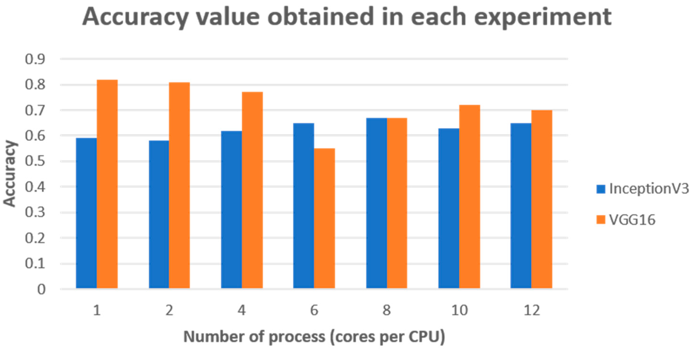
Our research results showed that in using the HPCC, we achieved a maximum accuracy of 82% with a training time of over 4 h, whereas the work of Olsen et al. [22] reported an average accuracy between 95.1% and 95.7% with a training time of 13 h using a single graphics card.

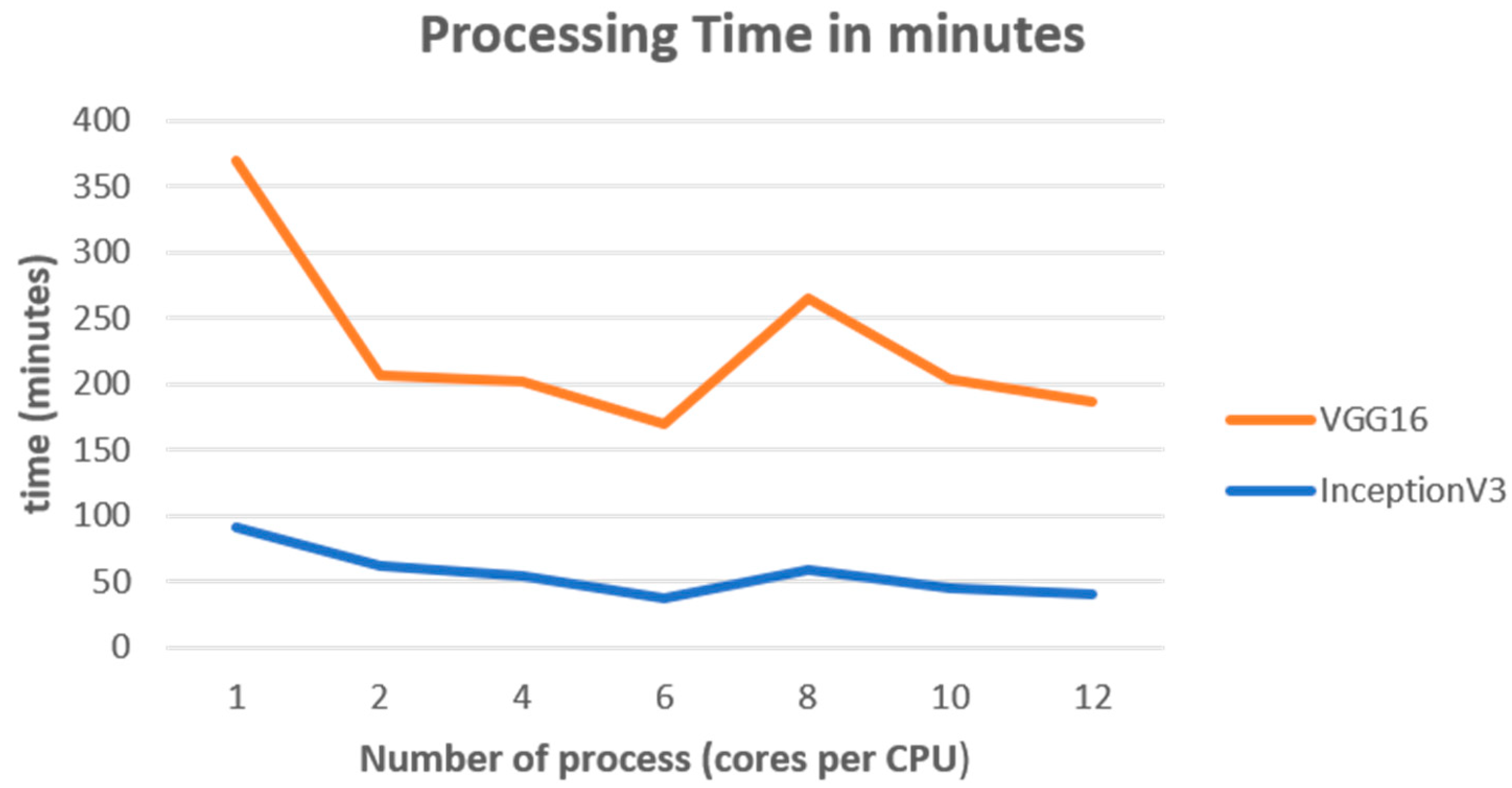
One of the critical metrics obtained in our research was accuracy, where we achieved the highest value of 0.82 using a single process in the proposed HPCC. However, the longer training times may have been due to the need for more epochs to achieve better loss values in the CNN VGG16 model. The number of epochs depended on the number of processes introduced to the HPCC, which explained why the metric values varied, as shown in Table 4, Table 5 and Table 6.

An interesting finding was that applying six processes in the HPCC resulted in the best time for both CNN models. Loading and distributing two processes as a parameter in each node, we were able to utilize 50% of the processor capacity in each computing node. This trend suggests that utilizing eight processes in an HPCC with additional computing nodes could yield even better processing times.

Finally, our research indicates that increasing the number of computing nodes could improve the model’s performance and execution times. Despite the limitations, our proposal offers a low-cost alternative that can be applied to different research areas that require HPC, such as PDI and AI.

5. Conclusions

HPC is an accessible tool for the scientific and university communities. The implementation of an HPCC with the characteristics presented in this proposal helps to use a small budget to make use of HPC to provide solutions or develop projects that involve PDI and AI techniques in a distributed way in small laboratories and research centers. This project demonstrates the benefit of processing time (a reduction of more than 60%) and the accuracy that is obtained if an application development environment related to PDI and AI is implemented, which have become very important techniques today.

Although there are much larger high-performance infrastructures in the world than the one proposed in this article, not all people or the scientific community can access them, due to the high cost and low accessibility, unless a considerable sum of money is invested.

Based on the experience acquired, it can be added that in an HPCC network, the resources are a very critical and important part and are essential to guarantee efficient and secure communication between cluster nodes and with other network resources. HPCCs require a high-quality network infrastructure to function optimally and achieve the benefits of high-performance computing.

For this reason, in this project, an accessible infrastructure was proposed that considerably reduced processing times and efforts compared with using a single computer.

As future work, it is proposed to integrate new computing nodes and GPU acceleration, which, although NCCL was used together with OpenMPI to use the collective communication libraries, could only be used by the CPUs and not by the NVIDIA-integrated cards. Implementing GPU acceleration could further reduce the processing time and could test multiple CNN models that were not used in this project.