Abstract
To overcome the problems of low machine learning fault diagnosis rate and long consumption time of deep learning in rolling bearing fault diagnosis, an RFR-GA-BLS model is proposed. The model is validated by infrared images of rolling bearings to find the most representative features, the most suitable parameters and the best diagnostic rate. Based on the pre-processed infrared thermal images of the faulty bearing, 72 second-order statistical features were obtained as information for fault diagnosis. RFR considered the robustness of the features, and new sequences were obtained. BLS was optimized by GA for fault diagnosis. New sequence features were added to the model sequentially, one at a time. After satisfying the model conditions, the most appropriate number of features was selected as the first 20. The search results for the number of feature nodes, the number of feature node windows and the number of enhancement nodes for the BLS were 24, 19 and 544, respectively, and the fault diagnosis rate of 98.8889% was achieved. According to a comparison with CFR-GA-BLS, BLS, PSO-BLS and Grdy-BLS, our proposed model is more advantageous in the search for the best performance. The fault diagnosis accuracy is higher compared to SVM and RF. The speed of our proposed model is 207 times faster than 1DCNN and 10,147 times faster than 2DCNN.
1. Introduction
Most of the fault diagnosis of rolling bearings is based on vibration signals and acoustic emission signals. However, the acquisition of both signals is susceptible to the influence of the external environment; i.e., noise is easily collected. Therefore, it is very difficult to extract useful information [1,2,3,4]. In recent years, temperature signals have gradually received the attention of researchers. Infrared thermal imaging cameras can acquire infrared images and thus display the thermal characteristics of objects. Compared with the two signals discussed above, the temperature signal has the characteristics of non-contact, high sensitivity and real-time. Due to its strong advantages for test targets running at high speeds, some scholars have introduced it into the troubleshooting of mechanical equipment [5,6]. Therefore, using infrared images as a research object for rolling bearing fault diagnosis has certain advantages.
Regardless of the signal base, the essential series of processes for fault diagnosis consists of feature extraction, feature selection and fault diagnosis. There is much related research on traditional vibration signals and acoustic emissions. Zhang et al. extracted features from bearing vibration signals in the time and frequency domains and applied Multidimensional Scaling (MDS) for feature selection and finally obtained highly accurate fault diagnosis results by fusing a support vector machine (SVM) [7]. Sun et al. combined the 1 Dimension Convolutional Neural Network (1DCNN) and Long Short-Term Memory (LSTM) to avoid the errors caused by relying on expert experience and incomplete information in traditional feature extraction methods [8]. Tian et al. proposed a Multi-domain Entropy-random Forest (MDERF) method that fuses multi-domain entropy and random forest to extract the multi-domain entropy of the acoustic emission signal as a feature extraction method to extract the four entropies of the AE signal and used the random forest to complete the fault diagnosis [9]. Pham et al. two-dimensionally verified the diagnostic capability of the improved generative adversarial network (GAN) under unbalanced acoustic emission signals [10]. Motor Current Signature Analysis (MCSA) is widely used for motor fault diagnosis. Granda et al. obtained the current signal of induction motor by MCSA and used the Continuous Wavelet Transform (CWT) model of the squirrel-cage induction motor for broken bar diagnosis [11]. Juan et al. obtained the vibration signal and current signal of the motor, calculating the Power Spectral Density (PSD) and Fast Fourier Transform (FFT). The amplitudes at the frequencies of interest given by the theory were analyzed to provide reliable fault diagnosis results [12].
Usually, feature extraction from IR images and feature selection are the top priority to ensure the completion of the subsequent work. Currently, most research scholars use the method of manually extracting the grayscale features, extracting texture features of the image or parsing the image using image analysis methods. Liu et al. extracted texture features, moment features and modified entropy features for server fault diagnosis [13]. Thobiani et al. used a two-dimensional empirical mode decomposition (BEMD) which was used to enhance the infrared thermal image of the bearing, after which the second-order statistical texture features of the image were extracted, and feature selection was performed using Minimum Redundancy Maximum Relevance (MRMR) [14]. In addition, another feature extraction method is to train and learn the data using deep neural network models to obtain high-level feature representation in the data. This feature extraction method has better performance and generalization capability than the traditional manual feature extraction method. Choudhary et al. directly extracted the features of the image using the 2 Dimension Convolutional Neural Network (2DCNN) and showed significantly better diagnostic results compared to others [15]. He et al. addressed the situation of insufficient data samples by incorporating the convolutional auto-encoder (CAE) and enhanced convolutional neural network (ECNN) to extract deep features [16]. Wei et al. constructed an extended model of faulty samples by migration learning and deep convolutional generative adversarial network (DCGAN) to solve the small sample infrared image fault diagnosis [17]. Thus, it can be seen that the criteria for feature selection are either difficult to develop or difficult to understand. Even if the identified best features are selected, it is difficult to ensure the optimal and minimum number of features. So, the way of feature selection needs to be improved.
Whether the data features are extracted from the infrared images as a way to characterize the images or the deep features of the images are constructed directly using deep learning, the later articulated methods are basically like those used for vibration and acoustic emission signals. Choudhary et al. used decision tree (DT), linear discriminant analysis (LDA) and SVM for fault diagnosis of electric motors, respectively, and eventually SVM proved to be superior for diagnosis [18]. Glowacz used a nearest neighbor classifier and back propagation neural network for fault diagnosis of infrared images of electric drills [19]. Janssens et al. acquired infrared images to extract pixel points in the x- and y-axis directions of the pixel histogram, light moments and Gini coefficients as data features and finally classified them using a random forest (RF) model [20]. Li et al. used SoftMax for classification after 2DCNN [21]. In conclusion, machine learning and deep learning are heavily cited for infrared image troubleshooting of machinery or electricity. However, machine learning often possesses data dependency and poor generalization of the models. Deep models, on the other hand, are time-consuming, resemble a “black box” and do not have good explanatory power.
In 2018, Chen, C.L.P. proposed the Broad Learning System (BLS), which is a random vector function linked neural network. It contains only a single layer of hidden layers and is expanded incrementally in a transversal manner anytime when faced with a learning inaccuracy. It greatly solves the problem of long training time for deep learning [22]. Wang et al. extracted features describing temporal and spatial distribution from infrared images of power equipment and finally diagnosed them using BLS [23]. Zhang et al. used double-tree complex wavelets to decompose vibration signals of bearing faults, extracted sub-bands as feature vectors and finally completed fast fault classification using BLS [24]. Wang et al. proposed TSK-BLS, which can be calculated quickly and accurately by pseudo-inverse and symmetric methods and has good fault diagnosis advantages [25]. Therefore, the introduction of width learning into the field of fault diagnosis has some practical significance. However, the parameters of the network model can have an impact on the accuracy. The parameters provided by the original authors are used in the above application of BLS for fault diagnosis. Some BLS-based fault diagnoses are aimed at the internal algorithms, which all use manually set parameters, generally for test verification or manual experience, and do not guarantee the best accuracy. Yu et al. defined connection weight matrices for inter-class and intra-class graphs to improve the fault diagnosis accuracy considering the sameness between similar samples and the difference between different classes of samples [26]. However, their parameters are set to fixed values based on manual experience, which may miss the optimal accuracy. Therefore, it is very necessary work to perform an optimization search for the parameters.
Infrared thermal images often contain more complex and stronger noise than ordinary optical images due to factors such as spatial and temporal environment and detection equipment. Likewise, the temperature of the surrounding environment can interfere with the focused information of the image. Therefore, noise removal and other pre-processing efforts are necessary.
In view of the above research background and existing problems, this article proposes an RFR-GA-BLS fault diagnosis model. Firstly, a series of pre-processing such as grayscale map conversion, region of interest (RoI) acquisition, denoising and image segmentation are performed on the acquired infrared images. Then, the second-order statistical features are extracted using the grayscale co-occurrence matrix (GLCM). After that, they are imported into RFR-GA-BLS. The extracted features are ranked by composing Robust Feature Ranking (RFR) with robust feature properties. The optimal features are added one at a time, and a feature search is performed to derive the optimal and minimum number of features. The optimal features and the highest accuracy of each round are filtered out after each round of data input to BLS using the optimization-seeking property of the Genetic Algorithm (GA).
The rest of the article is organized as follows: Section 2 introduces the relevant technical theory. Section 3 reviews the rolling bearing infrared image data acquisition experiments. Section 4 describes the model building. Section 5 gives the experimental results of fault diagnosis. Section 6 draws conclusions.
The contributions of this article are as follows:
- The infrared image replaces the previous vibration signal and acoustic emission signal, so that the fault performance is visualized.
- RFR uses the robustness of features to rank features in the RFR-GA-BLS fault diagnosis model. Instead of the previous way of filtering or rejecting features, it solves the problem of difficult feature selection by finding the optimal number of features and corresponding features in an iterative way.
- The GA-BLS in RFR-GA-BLS fault diagnosis model solves the problem of difficult setting of BLS parameters and can find the best parameters and the highest accuracy rate.
- RFR-GA-BLS has superior accuracy than machine learning and faster training time than deep learning.
2. Materials and Methods
2.1. GLCM and Second-Order Statistical Features
The second-order statistical features have a strong interpretation and good robustness, which can reflect the characteristics of the pictures more comprehensively [14]. It can be obtained by GLCM, which can be defined as:
where denotes the probability of occurrence of pixels with grayscale values i and j at the positions of phase and angle . denotes the number of pixels with grayscale values i and j at the positions of phase and angle . G denotes the number of grayscale levels of the image, i.e., 256.
Pixel distances of 1, 2 and 3 were chosen, respectively. Some 0°, 45°, 90° and 135° pixel angles were selected. The extracted second-order statistical features contain energy, contrast, entropy, sum average, variance and correlation. A total of 72 features are noted as GLCM_0, GLCM_1, … and GLCM_71. The extracted second-order statistical features are shown in Table 1.

Table 1.
Extracted second-order statistical features.
2.2. RFR
Features with robustness can reduce the effect of data outliers and noise and improve the stability of the classifier. An RFR method is given which exploits robustness and ranks features according to size. Thus, the most robust features are utilized in preference. Here, the robustness calculation metric is calculated using Mean Absolute Deviation (MAD), a measure of how discrete the data are. Larger values of MAD indicate more robust data, i.e., more tolerant of noise or outliers.
Robustness is used to assess the stability of the feature column in the face of outliers. Unlike other studies, after calculating the robustness metric of the feature column, the features with poor robustness performance are not eliminated or retained with good robustness performance. Instead, they are ranked according to the magnitude of the robustness values. The features GLCM_0, GLCM_1, … and GLCM_71 are ranked according to the 72 evaluation metrics obtained.
When performing fault diagnosis, the first diagnosis uses the first feature, which is the feature with the best robustness. The second diagnosis uses the first two features and so on, adding one new feature at a time until all 72 features have been taken.
2.3. GA
GA is an optimization algorithm that follows the principles of survival of the fittest and meritocracy. It is developed by borrowing from the genetic process in evolutionary biology. A series of operations such as inheritance, mutation, crossover and natural selection are included in it.
The genetic algorithm generates an initial population for the parameters to be optimized and evaluates it according to the fitness function. Thus, the set of solutions with small fitness function is eliminated, and the population with high fitness is retained. After operations such as amplitude, crossover and variation, the individuals are continuously preferred to obtain the optimal solution.
2.4. BLS
BLS is a random vector function linked neural network. By calculating the weights of feature nodes and augmentation nodes through pseudo-inverse operation, the calculation speed and measurement accuracy of the model can be improved comprehensively. The structure diagram is shown in Figure 1.
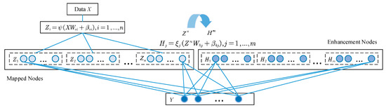
Figure 1.
The structure diagram of BLS.
First, the model completes the mapping of the input data to the feature nodes, which can be defined as:
where Zi is the i-th feature node; Wei is the random weight of the feature mapping layer; βei represents the random bias of the feature mapping layer.
The generation of augmented nodes from mapped nodes after transformation can be defined as:
where Hj is the j-th enhanced node; Whj is the random weight of the feature mapping layer; βhj represents the random bias of the feature mapping layer.
Output all mapped and enhanced nodes, which can be defined as:
where Y is the node set; represents the mapping node set; presents the enhancing node set; Wm represents the weight set.
Finally, the pseudo-inverse is then calculated to give the weights of the output layer, which can be defined as:
Therefore, it is very essential to set the number of feature nodes, the number of feature node windows and the number of enhancement nodes in the whole model. Here, they are denoted as N1, N2 and N3, respectively. In general, these parameters need to be manually tuned to achieve a high standard of diagnostic results. However, such a model does not have the ability to generalize and does not necessarily guarantee that the optimal diagnostic rate is obtained. Therefore, parameter optimization is necessary for N1, N2 and N3.
3. Experiment
The infrared image signal applied in this article comes from the rolling bearing failure experimental bench in Figure 2a. The intercepted IR video interface is shown in Figure 2b. The experimental bench includes a servo motor, controller, coupling, shaft, faulty bearing and an infrared thermal image acquisition system. The bearing model is S6205-2RSR. The motor speed is stabilized at 2000 rmp. The IR thermal image acquisition system includes BM_RI Software V7.4 and the IR thermal imaging camera FLIRA35. The parameters of the IR thermal imaging camera and the acquisition system are shown in Table 2.
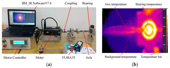
Figure 2.
Infrared image acquisition device and data acquisition interface. (a) The rolling bearing fault test bench; (b) Infrared video recording interface.
Table 2.
Infrared thermal imaging camera and acquisition system parameters.
In order to test the performance of the proposed model, nine states of the bearing are set. They are health condition (HE), holder failure (HO), inner ring 0.5 mm crack (IN05), inner ring 1.0 mm crack (IN10), inner ring 1.5 mm crack (IN15), outer ring 0.5 mm crack (OU05), outer ring 1.0 mm crack (OU10), outer ring 1.5 mm crack (OU15) and rolling ball pitting (RO).
During the acquisition process, the ambient temperature was maintained at about 24.5 °C. Each bearing state was waited for the temperature to remain stable while video acquisition was performed. Subsequently, 15 min of infrared video was acquired. The steps of infrared thermal image acquisition are shown below:
Step 1: A state bearing is mounted to the shaft.
Step 2: Turn on the motor controller and make sure the bearing is running at a constant speed of 2000 rmp.
Step 3: Observe the temperature change and start collecting infrared video for 15 min after it is roughly stable.
Step 4: Cool the rolling bearing failure test bench to ambient temperature of 24.5 °C.
Step 5: Repeat steps 1–4 to complete the acquisition of a total of nine 15 min infrared videos of different bearing failures.
Step 6: Extract infrared images from the videos according to the 9 s time interval, 100 images for each category. In total, 900 images were extracted.
Step 7: Select the bearing and shaft areas that produce temperature changes and crop them to obtain the RoI. The RoI of the extracted IR images for each category of bearings is shown in Figure 3.
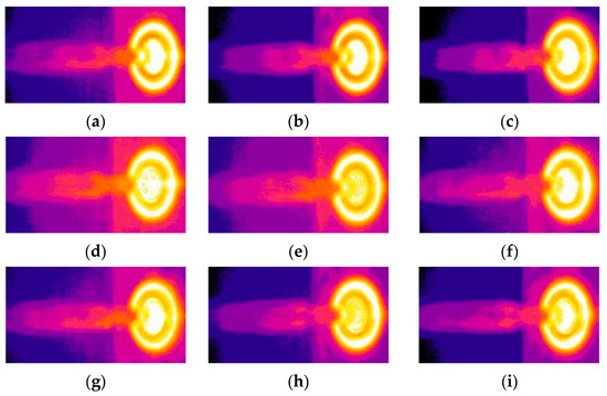
Figure 3.
RoI in infrared images of each bearing fault type (a) HE; (b) HO; (c) IN05; (d) IN10; (e) IN15; (f) OU05; (g) OU10; (h) OU15; (i) RO.
4. Fault Diagnosis Model
4.1. RFR-GA-BLS Fault Diagnosis Model
The flow chart of the proposed RFR-GA-BLS fault diagnosis model is shown in Figure 4.
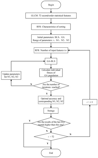
Figure 4.
RFR-GA-BLS fault diagnosis model.
The outermost side of the model is the RFR method. It sorts the 72 features by calculating the robustness of each column of features. The first loop selects the first feature at the top of the ranking. The second loop selects the second feature at the top of the ranking, and one is added in each loop until all 72 features are selected. In addition, a way to jump out of the loop is designed. Once the accuracy of a certain time exceeds 85% and the next four features are not as high as this one, it is determined that this is the best result found. All results are output at this point.
The middle part is the GA optimized BLS model. The fault diagnosis accuracy of the BLS model is used as the fitness function. N1, N2 and N3 are used as the optimization parameters. After setting the parameter ranges of N1, N2 and N3 and generating the initial population, the initial population is first subjected to fitness calculation, and the dominant individuals are selected for retention. The left individuals are subjected to a series of genetic operations to generate offspring. In the continuous evolution, the remaining offspring have increasing fitness, and thus the optimal solution that meets the objective is selected.
The remaining parameters were chosen as follows: for RFR, i from 1 to 72. For GA, the initial population N = 30; the spatial dimension d = 3; the maximum number of iterations ger = 10; the crossover probability Pc = 0.8, and the variation probability Pm = 0.1. For BLS, the shrinkage factor of the augmented nodes was s = 0.8; the regularization parameter was C = 2–20, and the range of N1 was [10, 30]; the range of N2 is [10, 30]; the range of N3 is [500, 600], and the step length is 1.
4.2. Fault Diagnosis Process
In this article, rolling bearing fault diagnosis based on infrared images is studied. Firstly, the infrared videos of nine kinds of faulty bearings are acquired, so as to crop the infrared images. After that, a series of pre-processing work such as RoI acquisition, grayscale image conversion, image denoising and image segmentation are performed. After completing these tasks, GLCM is applied to extract features. Finally, the acquired feature set is fault diagnosed using RFR-GA-BLS. The steps are as follows:
Step 1: Acquisition of IR images. IR video of nine types of rolling bearings were acquired for 15 min after temperature stabilization: i.e., HE, HO, IN05, IN10, IN15, OU05, OU10, OU15 and RO. IR images were cropped at 9 s intervals. Some 900 images can be obtained.
Step 2: Cropping images. The temperature of the bearing and the axis affected by the bearing temperature can be acquired as RoI. The 280*150 pixel area is set.
Step 3: Grayscale image conversion.
Step 4: Median filtering to remove noise. The size of the filter is set to 3*3, and the median is taken as the value of a certain pixel point.
Step 5: Adaptive thresholding segmentation. The image is transformed into a binary image. Firstly, a Gaussian weighted average is applied to set the threshold value, and the filter size is set to 5*5. Each pixel point is processed according to the obtained threshold value; pixels larger than the threshold value are 255, and pixels smaller than the threshold value are 0.
Step 6: Extraction of features. Extract the image features using GLCM, which contains energy, contrast, entropy, sum average, variance and correlation, with designed pixel distances of 1, 2 and 3 and angles of 0°, 45°, 90° and 135°, respectively. There are 72 features in total.
Step 7: Fault diagnosis. The obtained 72 features are input into the RFR-GA-BLS fault diagnosis model. Finally, the optimal features, the best parameters and the highest accuracy are obtained.
5. Results and Discussion
The specific experimental environment for completing the data dimensionality reduction and fault diagnosis stages on the Windows 10 operating system is shown in Table 3.
Table 3.
Experimental Environment.
After completing steps 1–5 of the fault diagnosis steps, the results are shown in Figure 5.
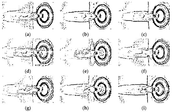
Figure 5.
Results after adaptive threshold segmentation (a) HE; (b) HO; (c) IN05; (d) IN10; (e) IN15; (f) OU05; (g) OU10; (h) OU15; (i) RO.
Subsequently, the 72 features, GLCM_0, GLCM_1, … and GLCM_71, were extracted using GLCM. Two fault diagnosis models, RFR-GA-BLS and CFR-GA-BLS, are applied to diagnose the faults, respectively. The RFR method and correlation feature ranking (CFR) are applied to rank these features, respectively, where the CFR method is the comparison scheme set up, based on the correlation of the features. It is obvious that these two feature ranking methods have a very different order for the ranked features. After sorting, the datasets were divided in a ratio of 9:1. Totals of 90 of each class were used as the training set and of 10 as the test set.
Additionally, then the GA-BLS model is set up in turn. For each round of feature increase, the training accuracy and test accuracy are saved, and the results are shown in Figure 6.
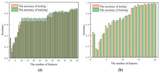
Figure 6.
Fault diagnosis accuracy (a) CFR-GA-BLS; (b) RFR-GA-BLS.
Figure 6a indicates the running results of CFR-GA-BLS. The first 55 features satisfy the algorithm conditions, and the final fault diagnosis accuracy obtained is only 0.86667. Figure 6b indicates the running results of RFR-GA-BLS. The final fault diagnosis accuracy obtained is 0.98889 for the first 20 features. In addition, the derived time variation is shown in Figure 7. The specific optimization-seeking parameters and corresponding results are shown in Table 4.
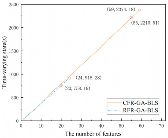
Figure 7.
Time-varying state of CFR-GA-BLS and RFR-GA-BLS.
Table 4.
Fault diagnosis results.
Figure 7 shows the time consumed for each feature addition. The CFR-GA-BLS satisfies the end condition only because of the first 55 features screened. Therefore, its running time is included in the next four diagnoses, which are used as a comparison diagnostic rate for skipping out of the loop. Its total run time is 2374.18 s. Similarly, the run time of RFR-GA-BLS is 918.28 s, which is about 15 min. Its speed is much smaller than that of CFR-GA-BLS, which is about 2/5. Table 4 lists the model run time, accuracy, number of features and parameters. Compared with CFR-GA-BLS, RFR-GA-BLS can apply a shorter time to show the best results, and its final selected features are the top 20. After optimization by GA, N1, N2 and N3 are 24, 19 and 544, respectively. Figure 8 illustrates the confusion matrix of RFR-GA-BLS. It clearly shows the distinction between the categories that generate errors. A sample that should belong to the OU10 category is incorrectly distinguished as OU05.
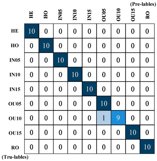
Figure 8.
Confusion Matrix for RFR-GA-BLS.
To determine whether the features, parameters and accuracy found by RFR-GA-BLS perform well, the model state was manually changed to remove the jump-out condition and run 72 times. The features sorted by CFR and RFR were sequentially imported into GA-BLS, and the change in accuracy was observed for each round, and the results are shown in Figure 9. The running time of each round of GA-BLS was exported, and the results are shown in Figure 10.
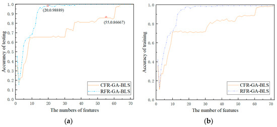
Figure 9.
Fault diagnosis accuracy of all features (a) CFR-GA-BLS; (b) RFR-GA-BLS.
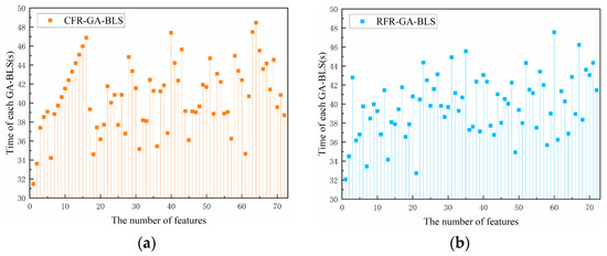
Figure 10.
Running time of each GA-BLS (a) CFR-GA-BLS; (b) RFR-GA-BLS.
According to Figure 9, it can be concluded that the CFR-GA-BLS model satisfies the end condition at the first 55 features, but its accuracy does not reach the optimal value. After the number of features is 65, the accuracy rate jumps. In the case of RFR-GA-BLS, the condition is satisfied at the number of features 20. Although 25 features can reach 1, 20 features make its operation time shorter, and the smaller accuracy gap can be ignored. Therefore, RFR-GA-BLS can achieve more efficient and accurate fault diagnosis.
Figure 10 shows the running time of each GA-BLS. It can be observed that adding a few features does not increase the GA-BLS operation time, and the running time is kept within 30–50 s. Therefore, width learning has great advantages as an optimization model.
In addition, this article verifies the superiority of GA-BLS. In order to reduce time consumption, only the first 20 features obtained in the previous experiments are selected for fault diagnosis. The comparison method was set up for comparison, as shown in Table 5.
Table 5.
Comparison of the operating results of the method.
The BLS model was chosen with the parameters of the code shared by the original authors, i.e., N1 = 10, N2 = 10, N3 = 500. The optimal accuracy obtained was 0.93333 with a running time of 0.18 s. Particle Swarm Optimization (PSO) was applied to determine the three parameters of the BLS model, and the number of iterations was again chosen to be 10. The accuracy is 0.97778, and the running time is 39.20 s. The Grdy-BLS using greedy algorithm (Grdy) to optimize the BLS obtains an accuracy of 0.95556 and the running time is 5.83 s.
Although the BLS model has a short running time, the accuracy of the model is low due to the poor generalization ability of the model by using only the parameters provided in the original text. PSO-BLS consumes slightly less time than GA-BLS, but the time difference is not significant. Its accuracy is lower than that of GA-BLS. Grdy-BLS has a short computing time, but the greedy algorithm tends to fall into a local optimum. As seen, the three parameters chosen fluctuate only in the initial state.
Therefore, GA-BLS is a good choice. As part of RFR-GA-BLS, it shortens the operation time and does not easily fall into the local optimum. Not only the good parameters and the minimum number of features are found, but also the optimal accuracy is obtained.
Subsequently, the first 20 features were used for fault diagnosis using SVM and RF. As shown in Table 6, SVM and RF are inferior to BLS in terms of speed and accuracy. The running time of SVM is 3.32 s, and that of RF is 2.19 s, which is faster but difficult to compare with BLS, and the algorithm will be exponentially higher if optimization parameters such as GA are added.
Table 6.
Comparison of broad-learning, machine-learning and deep-learning methods.
In addition, 1DCNN and 2DCNN were applied for fault diagnosis of infrared images. The top 20 features of the ranking were processed using 1DCNN, using two layers of convolution and two layers of pooling. The epoch was chosen to be 100. The speed was similar to that of GA-BLS, but only an accuracy of 0.9333 was obtained. The 2DCNN was used to process the image after adaptive thresholding, using two layers of convolution and two layers of pooling. The epoch was chosen to be 30. Still following the 9:1 dataset partitioning. Although it achieves an accuracy of 0.9889, it takes 10,147 times longer than BLS. The speed is also much slower than RFR-GA-BLS.
Thus, GA-BLS not only achieves the parameter search, but also has more advantages in terms of speed and accuracy. The problem of low accuracy of traditional machine learning fault diagnosis is overcome, and the problem of time-consuming deep learning of direct image processing is also overcome. The RFR-GA-BLS proposed in this article has strong advantages in the field of infrared image fault diagnosis of bearings.
6. Conclusions
In this article, an RFR-GA-BLS model is proposed and is applied to the infrared fault diagnosis of bearings. The model can obtain the optimal parameters and minimum features while achieving high standard fault diagnosis. The innovations of this article are as follows:
- The infrared images of rolling bearings are collected as the original signals for fault diagnosis, and the visualization of faults is realized.
- There is a changing the previous feature selection method and replacing it with RFR feature sorting. Thus, the problem of too much or too little feature selection is avoided.
- Optimization of BLS by using GA to obtain three parameters, N1, N2 and N3, and the best accuracy was achieved, combined with RFR fusion into RFR-GA-BLS fault diagnosis model to obtain the optimal number of features.
After experimental comparison, the RFR feature ranking method is obviously better than others. The GA-BLS optimization algorithm can achieve fast and accurate fault diagnosis. The infrared fault diagnosis of bearings using RFR-GA-BLS has certain advantages.
However, in this article, only the parameters of the BLS are optimized, and no improvements are made to the internal BLS. In addition, in real life, the bearing failure data are mostly unbalanced. Therefore, the data design aspect needs to be improved. The BLS also needs to be improved according to the data distribution problem. These are all issues that need to be addressed in subsequent studies.
Author Contributions
Conceptualization, L.L. and J.Z.; methodology, L.L.; software, L.L.; validation, L.L., X.S. and X.Y.; formal analysis, X.Y.; investigation, X.S.; resources, X.S.; data curation, L.L.; writing—original draft preparation, L.L. and J.Z.; writing—review and editing, X.S. and X.Y.; visualization, X.S.; supervision, X.Y.; project administration, L.L.; funding acquisition, J.Z. All authors have read and agreed to the published version of the manuscript.
Funding
This research was funded by the National Natural Science Foundation of China, grant number 51865010, and the Science and Technology Project of Jiangxi Provincial Department of Education, grant number GJJ210639.
Institutional Review Board Statement
Not applicable.
Informed Consent Statement
Not applicable.
Data Availability Statement
Not applicable.
Conflicts of Interest
The authors declare no conflict of interest.
References
- Chen, P. Review on Fault Diagnosis Methods for Rolling Bearings Based on Vibration Signals. Bearing 2022, 6, 1–6. [Google Scholar]
- Li, S.M.; Guo, H.D.; Li, D.R. Review of vibration signal processing methods. Chin. J. Sci. Instrum. 2013, 34, 1907–1915. [Google Scholar]
- Tan, J.C.; Xu, W.L.; Wi, J.J.; Chen, J.Y.; Guo, F.P. Overview of Acoustic Emission Fault Signal Analysis Method for Rolling Bearings. Guangdong Chem. Ind. 2015, 42, 93–94. [Google Scholar]
- Cockerill, A.; Clarke, A.; Pullin, R.; Bradshaw, T.; Cole, P.; Holford, K. Determination of rolling element bearing condition via acoustic emission. J. Eng. Tribol. 2016, 230, 1377–1388. [Google Scholar] [CrossRef]
- Xu, Q.; Huang, H.; Zhou, C.; Zhang, X. Research on Real-Time Infrared Image Fault Detection of Substation High-Voltage Lead Connectors Based on Improved YOLOv3 Network. Electronics 2021, 10, 544. [Google Scholar] [CrossRef]
- Li, Y.B.; Wang, X.Z.; Si, S.B.; Du, X.Q. A New Intelligent Fault Diagnosis Method of Rotating Machinery under Varying-Speed Conditions Using Infrared Thermography. Complexity 2019, 2019, 2619252. [Google Scholar] [CrossRef]
- Zhang, M.; Yin, J.; Chen, W. Rolling Bearing Fault Diagnosis Based on Time-Frequency Feature Extraction and IBA-SVM. IEEE Access 2022, 10, 85641–85654. [Google Scholar] [CrossRef]
- Sun, H.B.; Zhao, S.C. Fault Diagnosis for Bearing Based on 1DCNN and LSTM. Shock. Vib. 2021, 2021, 1221462. [Google Scholar] [CrossRef]
- Tian, J.; Liu, L.; Zhang, F.; Ai, Y.; Wang, R.; Fei, C. Multi-Domain Entropy-Random Forest Method for the Fusion Diagnosis of Inter-Shaft Bearing Faults with Acoustic Emission Signals. Entropy 2020, 22, 57. [Google Scholar] [CrossRef] [PubMed]
- Pham, M.T.; Kim, J.M.; Kim, C.H. Rolling Bearing Fault Diagnosis Based on Improved GAN and 2-D Representation of Acoustic Emission Signals. IEEE Access 2022, 10, 78056–78069. [Google Scholar] [CrossRef]
- Granda, D.; Aguilar, W.G.; Arcos-Aviles, D.; Sotomayor, D. Broken Bar Diagnosis for Squirrel Cage Induction Motors Using Frequency Analysis Based on MCSA and Continuous Wavelet Transform. Math. Comput. 2017, 22, 30. [Google Scholar]
- Dorantes, J.J.S.; Prieto, M.D.; Redondo, J.A.O.; Rios, R.A.O.; Troncoso, R.D.J.R. Multiple-fault detection methodology based on vibration and current analysis applied to bearings in induction motors and gearboxes on the kinematic chain. Shock. Vib. 2016, 2016, 5467643. [Google Scholar]
- Liu, H.; Xie, T.; Ran, J. An efficient algorithm for server thermal fault diagnosis based on infrared image. In Proceedings of the 2017 International Conference on Cloud Technology and Communication Engineering (CTCE2017), Guilin, China, 18–20 August 2017; Volume 910. [Google Scholar]
- Thobiani, F.; Tran, V.; Tinga, T. An Approach to Fault Diagnosis of Rotating Machinery Using the Second-Order Statistical Features of Thermal Images and Simplified Fuzzy ARTMAP. Engineering 2017, 9, 524–539. [Google Scholar] [CrossRef]
- Choudhary, A.; Mian, T.; Fatima, F. Convolutional neural network based bearing fault diagnosis of rotating machine using thermal images. Measurement 2021, 176, 109196. [Google Scholar]
- He, Z.Y.; Shao, H.D.; Zhong, X.; Yang, Y.; Cheng, J.S. An intelligent fault diagnosis method for rotor-bearing system using small labeled infrared thermal images and enhanced CNN transferred from CAE. Adv. Eng. Inform. 2020, 46, 101150. [Google Scholar]
- Wei, B.; Zuo, Y.; Liu, Y.; Luo, W.; Wen, K.; Deng, F. Novel MOA Fault Detection Technology Based on Small Sample Infrared Image. Electronics 2021, 10, 1748. [Google Scholar] [CrossRef]
- Choudhary, A.; Goyal, D.; Letha, S.S. Infrared thermography-based fault diagnosis of induction motor bearings using machine learning. IEEE Sens. J. 2020, 21, 1727–1734. [Google Scholar]
- Glowacz, A. Fault diagnosis of electric impact drills using thermal imaging. Measurement 2021, 2021, 108815. [Google Scholar] [CrossRef]
- Janssens, O.; Schulz, R.; Slavkovikj, V.; Stockman, K.; Loccufier, M.; Walle, R.V.; Hoecke, S.V. Thermal image based fault diagnosis for rotating machinery. Infrared Phys. Technol. 2015, 73, 78–87. [Google Scholar] [CrossRef]
- Li, Y.; Gu, J.X.; Zhen, D.; Xu, M.; Ball, A. An Evaluation of Gearbox Condition Monitoring Using Infrared Thermal Images Applied with Convolutional Neural Networks. Sensors 2019, 19, 2205. [Google Scholar] [CrossRef]
- Chen, C.L.P.; Liu, Z.L. Broad Learning System: An Effective and Efficient Incremental Learning System without the Need for Deep Architecture. IEEE Trans. Neural Netw. Learn. Syst. 2018, 29, 10–24. [Google Scholar] [CrossRef] [PubMed]
- Wang, J.; Zhao, C.H. Broad Learning System Based Visual Fault Diagnosis for Electrical Equipment Thermography Images. In Proceedings of the 2018 Chinese Automation Congress (CAC), Xi’an, China, 30 November–2 December 2018; pp. 1632–1637. [Google Scholar]
- Zhang, W.X.; Xu, J.J.; Liu, W.J.; Wang, J.G. Fault Diagnosis of Bearing Based on Double Tree Complex Wavelet and Broad Learning System. Mach. Des. Manuf. 2022, 5, 201–204. [Google Scholar]
- Wang, X.; Wang, C.; Zhu, K.; Zhao, X. A Mechanical Equipment Fault Diagnosis Model Based on TSK Fuzzy Broad Learning System. Symmetry 2023, 15, 83. [Google Scholar] [CrossRef]
- Yu, C.Y.; Zhang, W.T.; Zhang, Q.H.; Chen, J.W.; Ouyang, F.H. Fault Diagnosis Method of a Rolling Bearing on EMD-AR and Improved Broad Learning System. Proc. CSEE 2023. [Google Scholar]


Disclaimer/Publisher’s Note: The statements, opinions and data contained in all publications are solely those of the individual author(s) and contributor(s) and not of MDPI and/or the editor(s). MDPI and/or the editor(s) disclaim responsibility for any injury to people or property resulting from any ideas, methods, instructions or products referred to in the content. |
© 2023 by the authors. Licensee MDPI, Basel, Switzerland. This article is an open access article distributed under the terms and conditions of the Creative Commons Attribution (CC BY) license (https://creativecommons.org/licenses/by/4.0/).