Article

Response Prediction for Linear and Nonlinear Structures Based on Data-Driven Deep Learning

1
Department of Disaster Mitigation for Structures, College of Civil Engineering, Tongji University, Shanghai 200092, China
2
Shanghai Construction Group Co., Ltd., Shanghai 200080, China
*
Author to whom correspondence should be addressed.
Appl. Sci. 2023, 13(10), 5918; https://doi.org/10.3390/app13105918
Submission received: 30 March 2023 / Revised: 6 May 2023 / Accepted: 8 May 2023 / Published: 11 May 2023

Abstract

:
Dynamic analysis of structures is very important for structural design and health monitoring. Conventional numerical or experimental methods often suffer from the great challenges of analyzing the responses of linear and nonlinear structures, such as high cost, poor accuracy, and low efficiency. In this study, the recurrent neural network (RNN) and long short-term memory (LSTM) models were used to predict the responses of structures with or without nonlinear components. The time series k-means (TSkmeans) algorithm was used to divide label data into different clusters to enhance the generalization of the models. The models were trained with different cluster acceleration records and the corresponding structural responses obtained by numerical methods, and then predicted the responses of nonlinear and linear structures under different seismic waves. The results showed that the two deep learning models had a good ability to predict the time history response of a linear system. The RNN and LSTM models could roughly predict the response trend of nonlinear structures, but the RNN model could not reproduce the response details of nonlinear structures (high-frequency characteristics and peak values).

1. Introduction

Earthquakes are a type of catastrophic natural disaster with high unpredictability, great destructiveness, and extensive dispersion, and pose a serious threat to human existence and development [1,2]. The ground motion during an earthquake is fairly complicated for an individual construction site. Ground motion is transmitted to the superstructure of a building through its foundation, which causes the vibration of the structure as a reaction. It leads to serious casualties, economic losses, urban functional damage, and other accidents. Therefore, it is crucial for the design and health monitoring of structures to analyze their responses and performance under seismic loads in order to identify the bearing capacity and dynamic characteristics of structures [3,4].
Structural vibration during earthquakes is a very complicated engineering problem that involves many factors, such as ground motion, the foundation type, and the structural system. The complexity of ground motion is manifested in randomness and multi-directivity. Ground motion is a complex form of space motion including six components. It is a multi-dimensional, non-stationary, and random process, and its size and changes over time are unpredictable. Second, the influence and transmission of seismic action by different types of foundation are extremely complicated. In addition, the structural nonlinear characteristics and non-structural components lead to complexity in a structural system. These uncertainties directly result in challenges with computational accuracy and cost for structural responses.
In recent decades, data-driven deep learning (DL) technology has developed rapidly, showing significant advantages, such as strong information-extraction ability and a fast processing speed. As an effective means to resolve complex engineering problems, it has been widely used in various disciplines [5,6,7]. Therefore, DL can be used as a powerful forecasting tool to predict the response of complex nonlinear structural systems, thus replacing or simplifying complex numerical analysis processes, to a certain extent. It provides a new way to solve the nonlinear vibration problem in seismic engineering.

1.1. Structural Response Analysis

Structural dynamic response analysis is key to ensuring the safe service of building structures during earthquakes, and it is also a key and difficult point of structural seismic design. In order to explore the dynamic characteristics, influencing factors, and control strategies for buildings during earthquakes, many academics at home and abroad have carried out a series of studies [8,9,10]. These investigations comprise seismic testing, theoretical analysis, and numerical analysis (as shown in Table 1).
Seismic testing usually uses a seismic simulator or shaking table to imitate the actual seismic dynamic environment, and is one of the most effective methods for studying the dynamic responses of structures [11,12,13]. Its benefits include reliable data, intuitive phenomena, and the ability to consider the complexity and uncertainty of actual structures. Nevertheless, there are some challenges with seismic testing, including high costs, high equipment requirements, limited test conditions, and model errors.
In order to overcome the deficiency of seismic test research, a series of theoretical analysis methods have been proposed. At present, the methods commonly used in the theoretical seismic response analysis of building structures are the static force method, response spectrum method, energy method, and push-over method [14,15,16]. These methods have the advantages of simple calculation and stable analysis results, so they are widely used in practical seismic design. However, these methods only investigate structural performance as a whole and cannot reflect the dynamic characteristics of a structure during the seismic process. They are not suitable for structures with complex forms.
The advancement of numerical technology has given structural dynamic response analysis strong technological backing during the 20th century. Numerical analysis typically discretizes a structure into small finite elements or discrete elements to predict the response by solving dynamic equations [17,18,19,20]. This method can simulate a variety of seismic conditions and consider the influence of various structural parameters (such as material properties, structural forms, etc.) while providing a wider range of structural data, such as displacement, stress, etc. However, the responses of various buildings differ substantially because of the strong nonlinear, aperiodic, and non-stationary properties of ground motion. Therefore, several numerical calculations are frequently required for different buildings, which results in significant computational cost. In addition, as the application scenarios become more and more complex, the accuracy and efficiency of numerical techniques face great challenges in engineering applications due to the limitations of grid division and complex structural forms [21].

1.2. AI in Earthquake Engineering

One of the most significant areas of scientific research has always been how to employ machine learning models to extract trustworthy, worthwhile, and accurate information from vast volumes of data. As a nonparametric modeling method, artificial neural networks (ANNs) are a powerful tool for solving a wide range of challenging nonlinear engineering problems, because they can approximate any linear and nonlinear functional relations with arbitrary precision [22,23]. Previous studies have shown that ANNs can be used to effectively extract potential mapping relationships from large datasets. They are widely used in the fields of structural engineering, ocean engineering, and bridge engineering [24,25,26].
In earthquake engineering, ANNs are used to efficiently identify the hidden causality from massive structured data for application in earthquake prediction, ground motion modeling, and structural response analysis [27,28,29,30]. Saba et al. [31] proposed a BAT-ANN model to predict earthquakes. On the basis of past earthquake data, the weight of the model can be updated by the bat algorithm (BA) so that the feed-forward neural network (FFNN) can predict future earthquakes. Sreejaya et al. [32] used an ANN and a large number of ground motion records to build a prediction model of ground motion intensity for active shallow crustal earthquakes in India. The input variables of the model were the magnitude (M), hypocentral distance (R), site condition (S), and flag for the region (f), and the output variables were 21 ground motion parameters (GMPs) in both the horizontal and vertical directions. Suryanita et al. [33] used label datasets from 47 cities in Indonesia (different building heights, soil conditions, and seismic locations) and a backpropagation neural network (BPNN) to predict the structural responses, such as displacement, velocity, and acceleration, of multi-story buildings with a fixed floor plan.
The RNN is a special kind of ANN for time-series or sequential data [34,35]. The model generates the prediction sequence from the input information, which is very suitable for the response prediction of nonlinear structures under random seismic loads. However, when dealing with lengthy or highly nonlinear sequence data, the RNN can suffer from problems, such as gradient vanishing or gradient explosion, which cause the model to cease learning. In order to overcome these problems, the concept of “gate” was added on the basis of the RNN, and the LSTM was proposed [36]. RNNs and LSTMs are widely used in predicting the fatigue life of materials, damage monitoring, stock price index forecasting in finance, credit card fraud risk forecasting, and so on. They also have good applications in the field of earthquake engineering. Jena et al. [37] used several indicators to assess the susceptibility of seismic wave amplification by predefined weights of layers, and then applied 10 indicators to a developed recursive neural network model to generate earthquake probability maps that allowed for earthquake probability estimation. Nicolis et al. [38] built a seismic rate prediction model for Chile by inputting earthquake data into a LSTM and convolutional neural network (CNN). The above studies were attempts to use ANNs as a tool to solve nonlinear problems in seismic engineering. Their results indicate that a suitable ANN model can surpass traditional methods to predict complex structural responses. At present, with the application of energy dissipation technology and isolation technology, the structural responses to earthquakes have strong nonlinear, diversity, and other characteristics. How to use neural networks to capture these features is still a subject worthy of further research.
Inspired by the above summary, RNN and LSTM models are used to predict the response of structures with or without a nonlinear component (isolation technology) in this study. Based on the time series k-means (TSkmeans) algorithm, different acceleration records and corresponding structural responses (obtained by a numerical method) are divided into different label data clusters. The responses of nonlinear and linear structures under different seismic waves are predicted by trained models. The method can be used to monitor the health of structures with different structural vibration control techniques (such as isolation, energy dissipation, and dynamic vibration absorption technologies), which has great engineering application prospects.

2. RNN and LSTM Models for Structural Response Prediction

2.1. RNN Model

RNNs are a kind of neural network with short-term memory ability for processing and predicting sequence data. Different from the traditional deep neural network (DNN), the RNN adds a hidden state ht to connect the neurons in the hidden layers and has the ability to record information. As shown in Figure 1, the hidden unit ht is determined by the previous hidden unit ht−1 and the current input xt. The forward propagation process of RNNs can be expressed as:
h t = σ ( w x h x t + w h h h t 1 + b h ) y ^ t = σ ( w h y h t + b y )
where wxh, whh, and why are the weights, bh and by are the biased terms, and σ ( ) is the activation function. The back propagation algorithm is adopted to iteratively update parameters θ(w, b) in the model. The updated equation of the parameters is as follows:
θ new = θ old α θ J ( θ )
where α is the learning rate and θ J ( θ ) is the gradient.
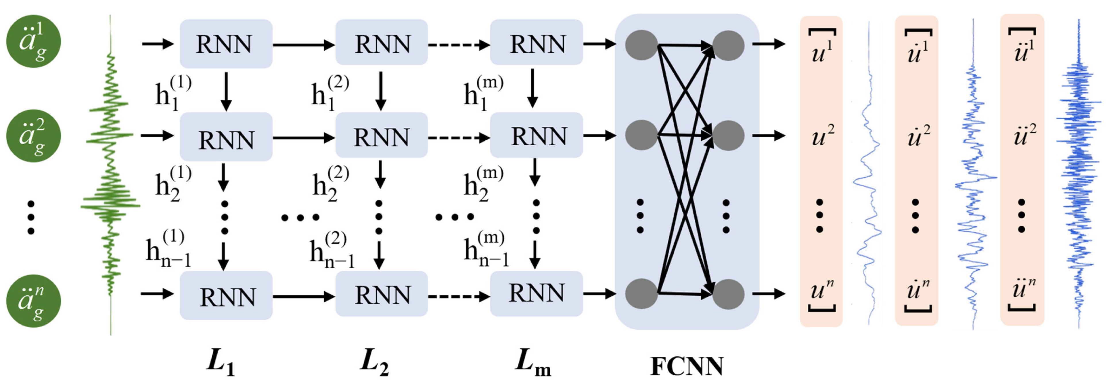
The linear and nonlinear characteristics of the structural system and different types of excitation inputs will affect the dynamic behavior of the structure. The response prediction models for linear and nonlinear structures during earthquakes were established based on the RNN model. The input of the model is the seismic wave sequence a ¨ g = [ a ¨ g 1 , a ¨ g 2 , a ¨ g 3 , , a ¨ g n ] and the output is the structural response [ u , u ˙ , u ¨ ] , as shown in Figure 2.

2.2. LSTM Model

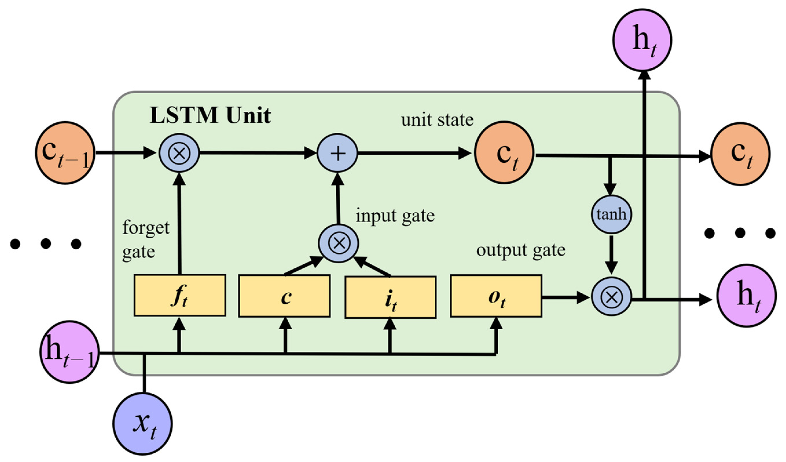
As shown in Figure 3, the LSTM unit adds three filter gates (forget gate, input gate, and output gate) to control the transmission and rejection of features based on the RNN model. This allows for the transmission and expression of information from a lengthy data sequence without the loss of important information from long ago. The LSTM is composed of a series of LSTM units. In each LSTM unit, the forget gate is used to decide whether to retain the unit state ct−1 of the t − 1 time step, and its output value ranges within [0, 1]. The input gate is used to update the unit state ct. The output gate is responsible for calculating the hidden state ht. The forward propagation process of the LSTM can be expressed as:
Input   gate :   i t = σ ( w i x x t + w i h h t 1 + b i ) Input   node :   c = tanh ( w c x x t + w f h h t 1 + b c ) Forget   gate :   f t = σ ( w f x x t + w f h h t 1 + b f ) Output   gate :   o t = σ ( w o x x t + w o h h t 1 + b o ) Unit   state :   c t = f t c t 1 + i t c Hidden   unit :   h t = o t tanh c t Output   layer :   y ^ t = σ ( w h y h t + b y )
where w i x , w i h , w c x , w f h , w f x , w f h , w o x , w o h , and w h y are the network weights, b i , b c , b f , b o , and b y are the bias terms, is the element-wise multiplication, and tanh is the hyperbolic tangent function.
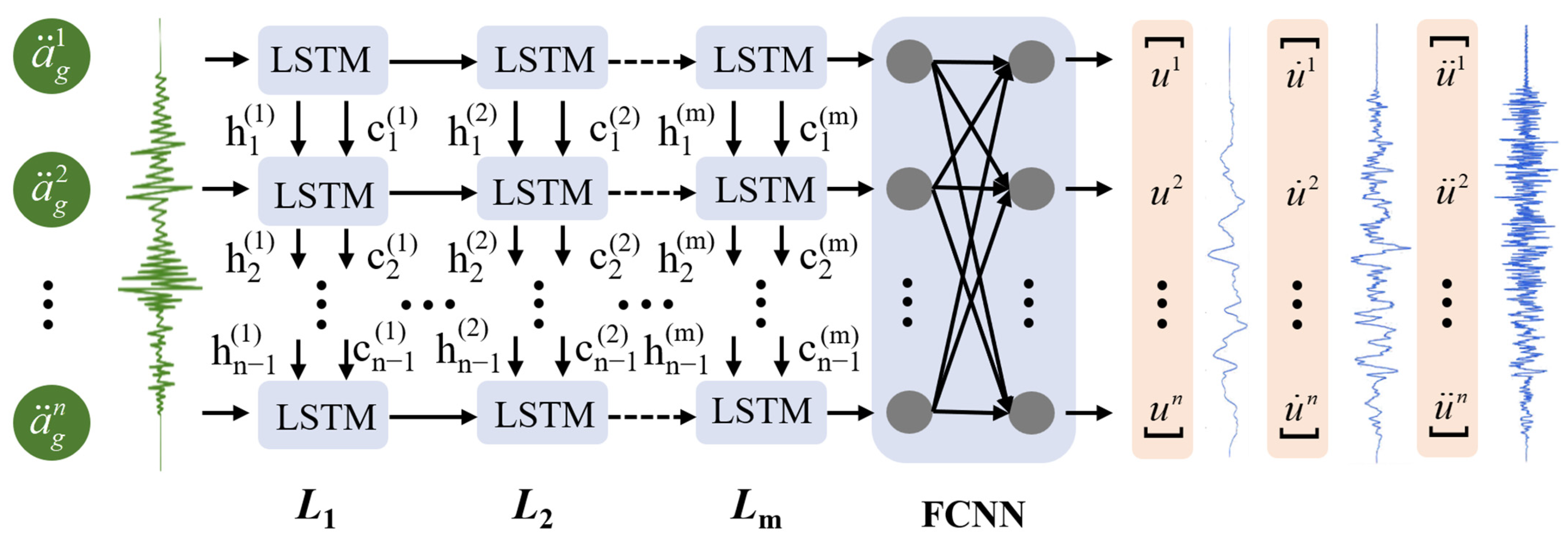
The LSTM model can be extended in both the vertical and horizontal dimensions and finally connected to the fully connected layer. Based on the LSTM, the response prediction models for linear and nonlinear structures under different seismic waves were established (see Figure 4). As in Section 2.1, the input of the models is the seismic wave sequence a ¨ g = [ a ¨ g 1 , a ¨ g 2 , a ¨ g 3 , , a ¨ g n ] and the output is the structural response [ u , u ˙ , u ¨ ] .

3. Construction of Dataset and Training of Models

3.1. Linear and Nonlinear Structural Models

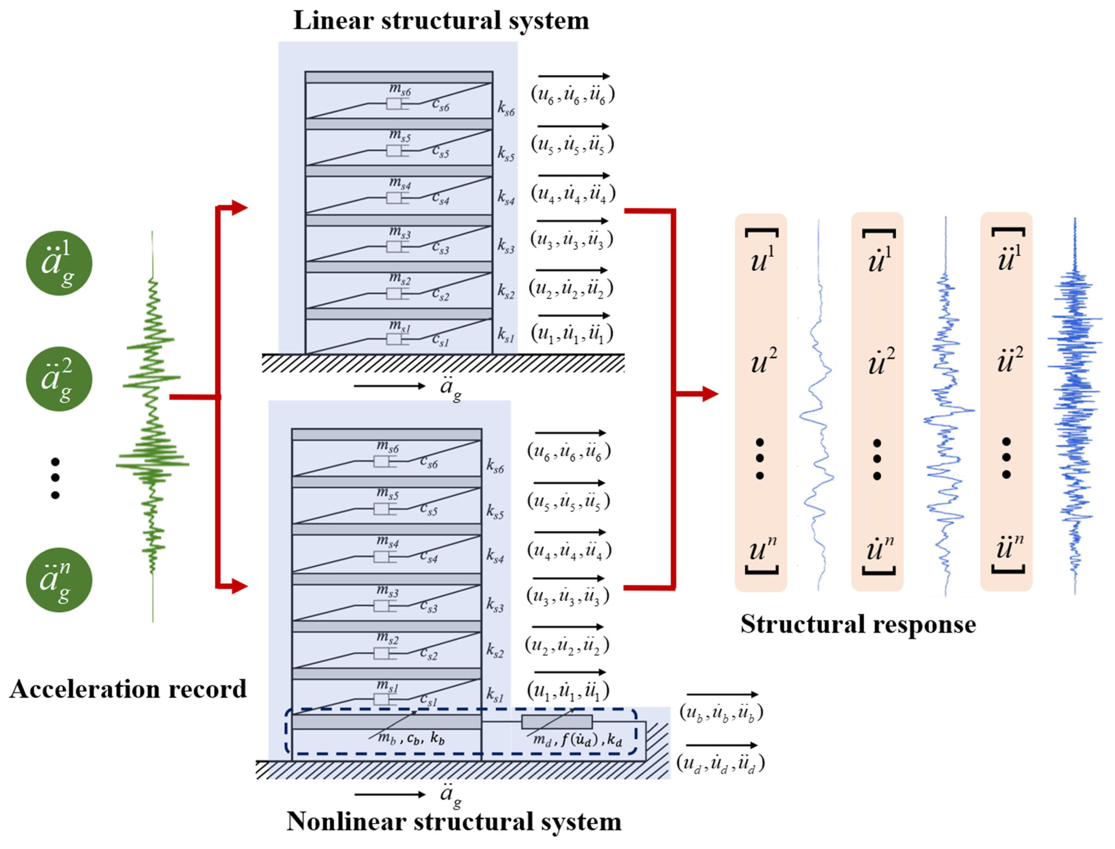
A six-story reinforced concrete frame structure was taken as the research object, which was simplified as a linear structure system with multiple degrees of freedom, as shown in Figure 5. A nonlinear structural system is established by adding a nonlinear component to the linear structural system.
The nonlinear component consists of two parts: the linear model mb and nonlinear model md. Its governing equation can be expressed as:
m s 1 u ¨ s 1 + c s 1 ( u ˙ s 1 u ˙ b ) + k s 1 ( u s 1 u b ) = m s a ¨ g m b u ¨ b + c b u ˙ b + k b u b [ c s 1 ( u ˙ s 1 u ˙ b ) + k s 1 ( u s 1 u b ) ] k d ( u d u b ) = m b a ¨ g m d u ¨ d + f ( u ˙ d ) + k d ( u d u b ) = m d a ¨ g
where the subscript s represents the superstructure, i is the floor number, b and d represent the linear and nonlinear models of the nonlinear component, m, c, and k are the mass, damping, and stiffness, respectively, a ¨ g is the ground acceleration, and u , u ˙ , and u ¨ are the displacement, velocity, and acceleration of the structure, respectively. The Rayleigh damping of the superstructure is 0.05. The detailed parameters of the structure are shown in Table 2 and Table 3.
The above two systems are solved by the Newmark-β method, and the structural responses [ u , u ˙ , u ¨ ] under different seismic waves are obtained. The governing equation of structural vibration can be expressed as:
M x ¨ + C x ˙ + K x = F
where M, C, K, and F represent the mass, damping, stiffness, and force, respectively, and x , x ˙ , and x ¨ represent the displacement, velocity, and acceleration, respectively. Based on the Newmark-β method, the structural response can be expressed as:
x ¨ t + Δ t = 1 β Δ t 2 ( x t + Δ t x t ) 1 β Δ t x ˙ t ( 1 2 β 1 ) Δ t x ¨ t x ˙ t + Δ t = γ β Δ t ( x t + Δ t x t ) + ( 1 γ β ) x ˙ t + ( 1 γ 2 β ) Δ t x ¨ t
where β and γ are parameters that control the accuracy and stability of numerical analysis, respectively, β = 0.5 and γ = 1 / 6 ; Δ t represents the time step, Δ t = 0.02 s. The structural response can be solved by combining the initial conditions and the governing equation.

3.2. Clustering of Seismic Waves Based on TSkmeans

3.2.1. Selection of Seismic Excitations

In order to increase the generalization of the ANN model, different seismic acceleration records were selected from NGA-West2 of the Pacific Earthquake Engineering Research Center (the selected acceleration records are shown in Table A1 of Appendix A). The selection principles of seismic waves were as follows:
  • The seismograph station is located on a free field or the ground floor of a low building;
  • Strong earthquake records with magnitudes above 5.5;
  • Velocity time history of seismic records with or without the pulse waveform;
  • Fault distance ranges from 0 to 100 km.
These actual acceleration records have different characteristics, such as near field, far field, and being with or without velocity pulse waveforms. The selected 60 acceleration records were resampled with a frequency of 50 Hz and a duration of 50 s. Each acceleration record was processed with baseline correction and low-pass filtering processing to mitigate edges and noise. The spectrum characteristics of the selected acceleration records are shown in Figure 6. By using incremental dynamic analysis (IDA), the amplitudes of 60 original acceleration records were adjusted, and 582 new acceleration records were generated. The different acceleration records generated by IDA based on the same original acceleration record had the same spectral characteristics.

3.2.2. Clustering of Seismic Records

In order to better extract the hidden features in the seismic sequence and reduce the dependence of the ANN model on the training dataset, this study uses the time series k-means (TSkmeans) algorithm to conduct cluster analysis of seismic records with different characteristics. The aim of the TSkmeans algorithm is to divide the sequence sets X = {X1, X2, …, Xn} (each sequence Xi = {xi1, xi2, …, xim} contains m time steps) into k clusters based on k clustering centers C = {C1, C2, …, Ck} (Ci = {ci1, ci2, …, cim}). The objective function of the TSkmeans algorithm is formulated as follows:
P ( U , C , W ) = p = 1 k i = 1 n j = 1 m u i p w p j ( x i j c i j ) 2 + 1 2 α p = 1 k j = 1 m 1 ( w p j w p ( j + 1 ) ) 2
Subject to
p = 1 k u i p = 1 , u i p { 0 , 1 } j = 1 m w p j = 1 , 0 w p j 1
where U is an n × k binary matrix, W = {W1, W2, …, Wk} is the weight matrix, and α is a balance parameter controlling the smoothness of the weights of time stamps, which can be expressed as:
α = i = 1 n j = 1 m ( x i j i = 1 n x i j n ) 2
The TSkmeans algorithm achieves the classification of time series by minimizing the objective function P(U,C,W). The main process is as follows:
  • Input: the sequence set X, the number of clustering centers k, the equilibrium parameters α , and the random initial values W and C.
  • Repeat:
    Step 1: Based on W and C, U is solved by the following formula:
    u i p = 1 ,   i f   D p j D p j , p p , 1 p k 0 ,   o t h e r w i s e
    where D p j can be expressed as:
    D p j = j = 1 m w p j ( x i j c p j ) 2
    Step 2: Based on the initial W and U obtained in step 1, C is solved by the following formula:
    c p j = i = 1 n u i p x i j i = 1 n u i p
    Step 3: U and C are obtained based on steps 1 and 2, and W is solved by quadratic programming.
  • Output: Determine convergence, output U, C, W.
Based on the TSkmeans algorithm, cluster analysis was performed on 60 original acceleration records according to the spectral characteristics, and the original seismic records and corresponding structural responses were divided into three cluster datasets by determining three cluster centers. The cluster centers are shown in Figure 7.

3.3. Input and Output of Neural Network Model

The training set used to train the ANN included 80% of the data randomly selected from the divided three cluster datasets. The remaining 20% of the data and 582 acceleration records obtained by IDA served as the test set. For the prediction models of the linear structure system, the input was a ¨ g = [ a ¨ g 1 , a ¨ g 2 , a ¨ g 3 , , a ¨ g n ] and the output was a response [ u s i , u ˙ s i , u ¨ s i ] i = 1 , 2 , 3 , 4 , 5 , 6 of layers 1–6. For the nonlinear structure system, the input of the models was a ¨ g = [ a ¨ g 1 , a ¨ g 2 , a ¨ g 3 , , a ¨ g n ] and the output was the response [ u s 6 , u ˙ s 6 , u ¨ s 6 , u b , u ˙ b , u ¨ b , u d , u ˙ d , u ¨ d ] of layer 6, linear component mb, and nonlinear component md. The input and output variables of each model are shown in Table 4. The server platform and environment configuration used for all model training in this study are shown in Table 5.

3.4. Model Training

3.4.1. Model Training for the Linear Structure

In order to eliminate the adverse effects caused by the singular sample data, the training set was normalized in the training process. Considering the training cost, training accuracy, underfitting, and overfitting, the hyper parameters of the RNN and LSTM models used to predict the linear structure are shown in Table 6 and Table 7. The mean square error (MSE) was selected as the precision evaluation index of model training, as follows:
L o s s = M S E = 1 n i = 1 n ( y i y ^ i ) 2
where y ^ i and y i represent the predicted and true values, respectively.
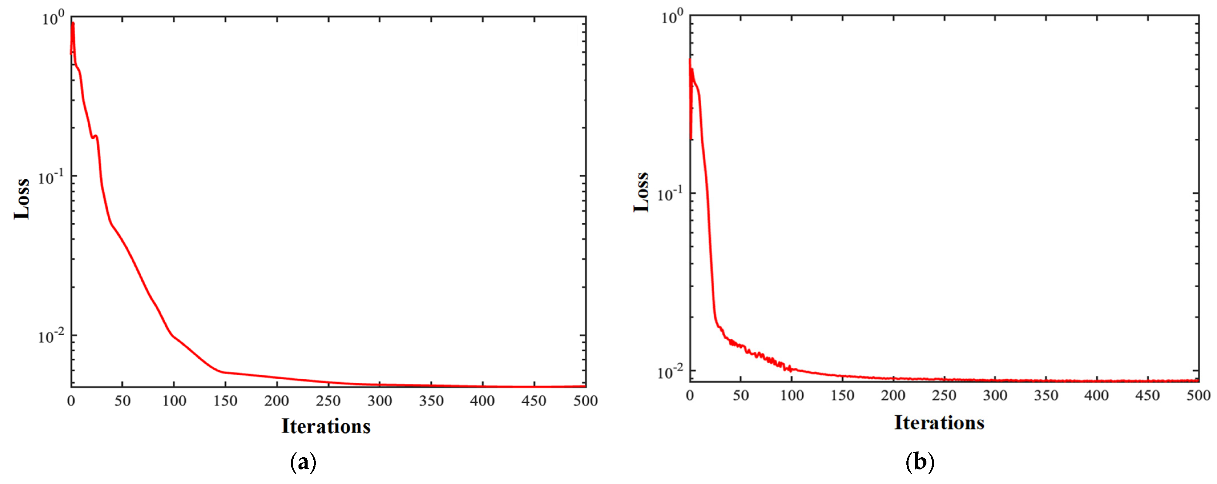
Figure 8a,b show the loss curves of the RNN and LSTM models used to predict the linear structural response in the training process, respectively. It can be seen that the loss curves of the two models converge to the threshold range at about 300 iterations. The convergence speed of the LSTM model was slightly faster than that of the RNN model.

3.4.2. Model Training for the Nonlinear Structure

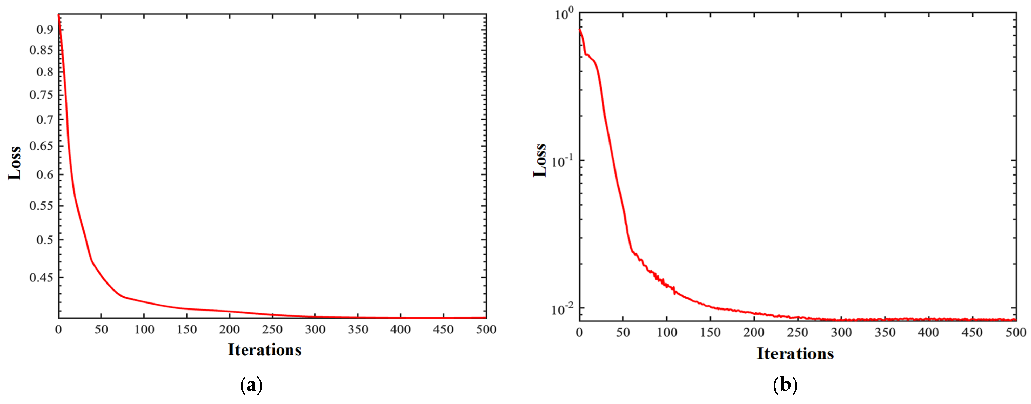
Considering the training cost, training accuracy, underfitting, and overfitting, the hyper parameters of the RNN and LSTM models used to predict the nonlinear structure are shown in Table 8 and Table 9. Figure 9a,b show the loss curves of the RNN and LSTM models used to predict the nonlinear structural response in the training process, respectively. The loss value is calculated as Equation (13).

4. Results and Discussion

4.1. Response Prediction for the Linear Structure

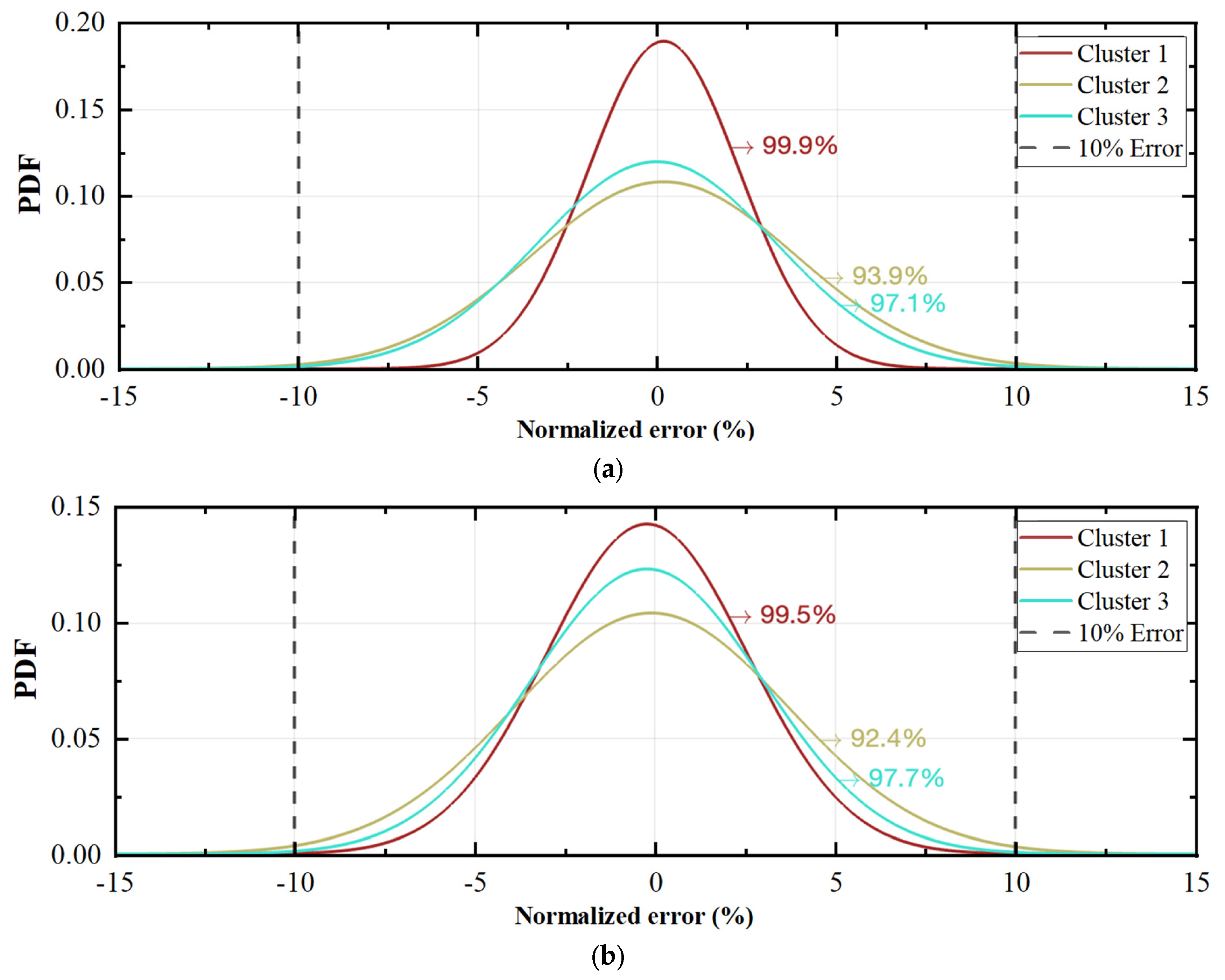
In this section, the trained RNN and LSTM models are used to predict the response of the linear system. The probability density function (PDF) Pi is used to analyze the error of the prediction results of the three cluster datasets in the test set. Pi is calculated as follows:
P i = P D F ( y i y i ) max ( y 1 , y 2 , , y n )
In order to further evaluate the prediction accuracy of the model, the weighted mean absolute percentage error (WMAPE) EWMAPE and peak percentage error (PPE) EPEAK were selected as evaluation indexes. The calculation formula is as follows:
E W M A P E = 1 m × n j = 1 m i = 1 n y i y i max ( y 1 , y 2 , , y n ) × 100 %
E P E A K = y p e a k y p e a k y p e a k × 100 %
where y p e a k is the true peak value of the time history response and y ^ p e a k is the predicted peak value of the time history response.
Figure 10 shows the error distribution of the prediction results by the RNN and LSTM models. As shown in Figure 10a, the errors of the result predicted by the RNN model were mainly distributed within the range of ±10%. Within this interval, the confidence degrees of the three clusters’ prediction results were 99.9%, 93.9%, and 97.1%, respectively. As can be seen from Figure 10b, the prediction results of the LSTM model had similar probability distributions to the RNN model, and the errors were mainly concentrated in [–10%, 10%]. The corresponding confidence degrees were 99.5%, 92.4%, and 97.7%, respectively. The error values of the predicted structural response under seismic waves in cluster 1 were more concentrated around 0. In general, the errors of the linear structural response predicted by the RNN and LSTM models were within a reasonable range. There was no significant difference in the response prediction results of the linear structure system under different types of seismic waves. The results demonstrate that the two models had high generalization and prediction accuracy.
Table 10 shows the error values EWMAPE and EPEAK of the results predicted by the RNN and LSTM models. EWMAPE was used to describe the accuracy of all the predicted results. It can be seen that the EWMAPE and EPEAK of the predicted results of the displacement u , velocity u ˙ , and acceleration u ¨ of different floors were all within 10%. According to the two indexes EWMAPE and EWMAPE, the RNN model had a good prediction effect on the global displacement response and peak value of the acceleration response. The LSTM model could also predict the global acceleration response and peak value of the displacement response well.
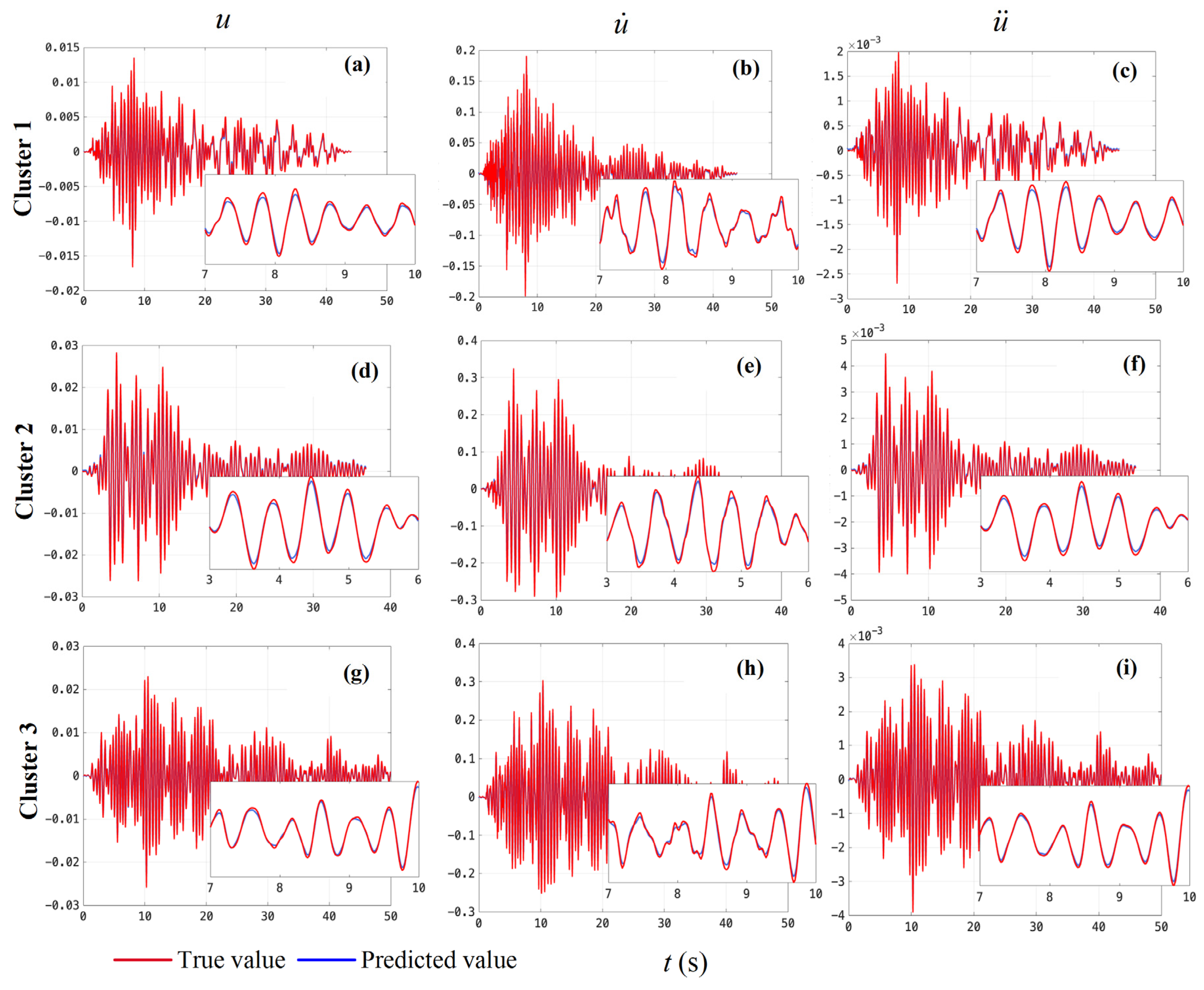
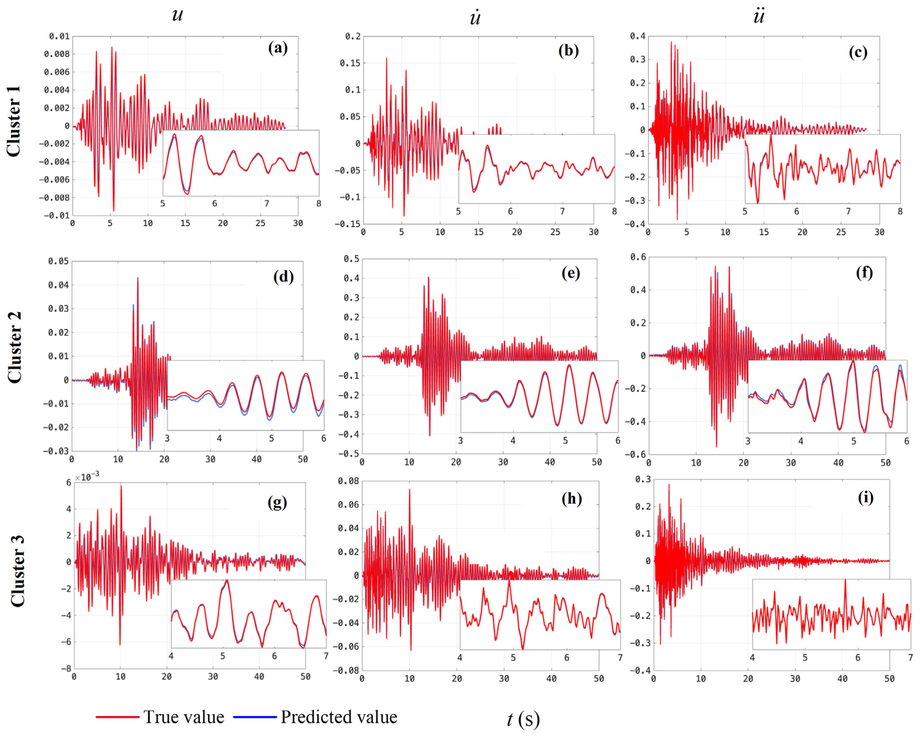
The response of the 3rd layer under the action of a seismic wave was randomly selected from the three cluster test sets for analysis. The comparison results of the predicted value and true value of the RNN and LSTM models are shown in Figure 11 and Figure 12, respectively. It can be seen that, for both the RNN model and the LSTM model, the predicted values of the displacement u , velocity u ˙ , and acceleration u ¨ responses of the linear system were highly consistent with the true values. As shown in Figure 11b and Figure 12h, the predicted results of the RNN and LSTM models were not only consistent with the actual velocity response trend on the whole, but also showed the characteristics of high frequency vibration locally. In addition, it can be seen that the prediction effect of the two models on the structural response under the action of the acceleration records in cluster 2 was slightly poor. The main reason for this phenomenon was that the acceleration records in cluster 2 had strong non-stationary characteristics (pulse characteristic). The nonlinear mapping capability of the neural network with a limited number of layers was insufficient, and some small nonlinear features and high frequency components could not be extracted.

4.2. Response Prediction for Nonlinear Structure

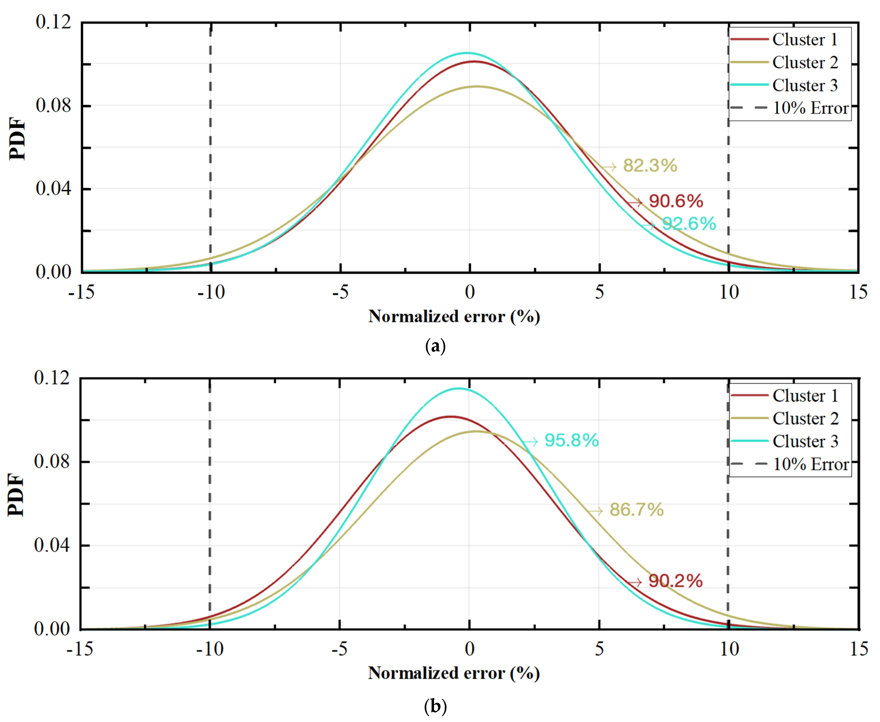
Figure 13 shows the probability distribution of the prediction results’ normalized errors of the RNN and LSTM models for the nonlinear structure. Within the confidence interval of [−10%, 10%], the confidence degrees of the three clusters’ responses predicted by the RNN model were 90.6%, 82.3%, and 92.6%, respectively, and the confidence degrees of the three clusters responses predicted by the LSTM model were 90.2%, 86.7%, and 95.8%, respectively. Compared with the predicted results for a linear structure, the prediction accuracy of the RNN and LSTM models for nonlinear structure responses was significantly decreased.
Table 11 shows the WMAPE EWMAPE and PPE EPEAK of the predicted displacement responses [ u s 6 , u b , u d ] of the top layer of the superstructure, linear model mb, and nonlinear model md. It can be seen that the WMAPE value of the nonlinear system response predicted by the RNN model was small, but the PPE value was large. The results show that, although the RNN model could roughly predict the response trend of the nonlinear structure, to some extent, it was very poor in predicting the peak value of the response. In addition, it could be found that the prediction error of the response to the nonlinear model md was significantly higher than that of the top-layer and linear models mb. That is to say, the RNN model could not learn the non-linear features of the response well. Table 12 shows the WMAPE EWMAPE and PPE EPEAK of predicted responses [ u ˙ d , u ¨ d , u b , u ˙ b , u s 6 , u ¨ s 6 ] . Similar to the prediction results of the RNN model, the prediction responses of the LSTM model also showed the trend of a small WMAPE value and large PPE value. However, compared with the RNN model, the prediction error of the LSTM model was significantly smaller. On the whole, the LSTM model had the worst prediction accuracy for the acceleration response peak value.
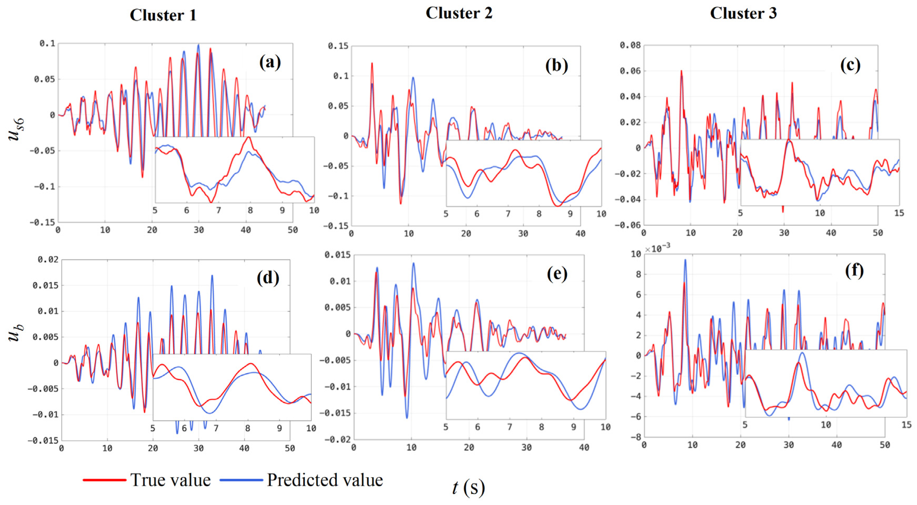
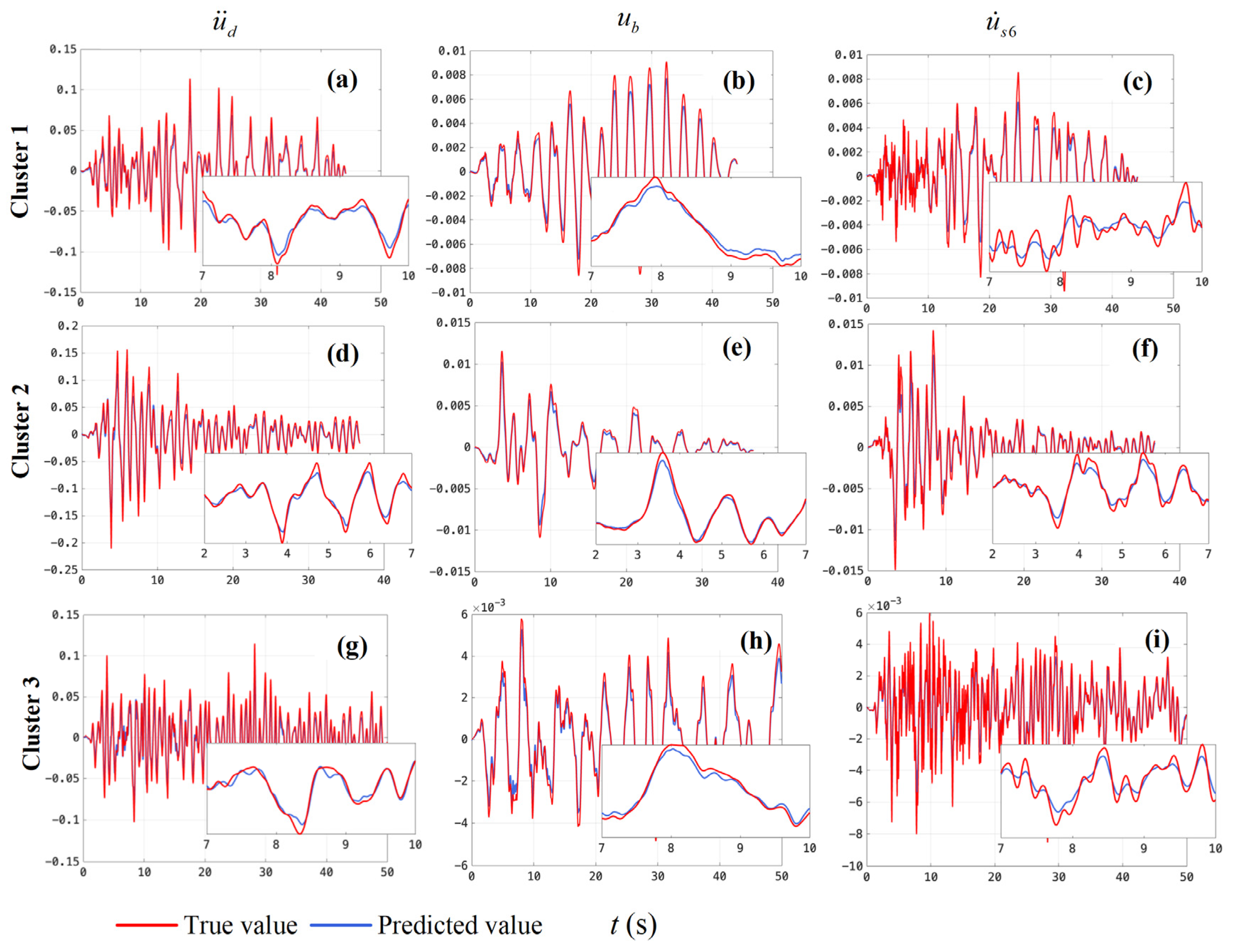
In order to further illustrate the prediction accuracy of the RNN and LSTM models for a nonlinear structural response, part of the prediction results and corresponding true values were randomly selected for comparison and analysis, as shown in Figure 14 and Figure 15. It can be seen from Figure 14 that the predicted results of the RNN model were consistent with the overall trend of the true value, but the prediction effect for some details was extremely poor (especially for the reproduction effect of high-frequency characteristics and peak values). The prediction effect of the LSTM model on the nonlinear structural response was significantly better than that of the RNN model (see Figure 15). As shown in Figure 15d,f, the LSTM model could reproduce the details of the response of the nonlinear structure well (although there was some error in the prediction peak value, it was within the allowable range).

5. Conclusions

In this paper, the RNN and LSTM models were used to predict the responses of linear and nonlinear structures, respectively. Through the IDA for 60 original acceleration records, 582 new acceleration records were generated. The structural responses of linear and nonlinear structures under different seismic waves were analyzed by a numerical method. On this basis, label data were constructed to complete the training of the model. The trained models were used to predict the responses of linear and nonlinear structures. The main conclusions were obtained as follows:
(1)
The RNN and LSTM models had good accuracy and generalization for predicting linear structural responses. Within the confidence interval [−10%, 10%], the confidence degrees of the prediction results by the RNN model for linear structural responses under the three clusters’ seismic waves were 99.9%, 93.9%, and 97.1%, and those of the LSTM model were 99.5%, 92.4%, and 97.7%, respectively. Both the overall trend and details of the linear structure responses predicted by the two models were highly consistent with the true values. Both the RNN and LSTM models were capable of predicting the response of linear structures under different seismic waves. In addition, it was found that the non-stationary characteristics of seismic waves could reduce the prediction accuracy of the models.
(2)
The overall accuracy of the RNN in predicting nonlinear structural response was poor. Compared with the predicted results of linear structures, the prediction accuracy of the RNN model for nonlinear structure responses was significantly decreased. Within the confidence interval [−10%, 10%], the confidence degrees of the three clusters’ responses predicted by the RNN model were just 90.6%, 82.3%, and 92.6%, respectively. The predicted results of the RNN model were consistent with the overall trend of the true value; however, the prediction effect for some details was extremely poor (especially in the reproduction of high-frequency characteristics and peak values).
(3)
The performance of the LSTM model was significantly better than that of the RNN model in predicting nonlinear structural responses. Within the confidence interval [−10%, 10%], the confidence degrees of the three clusters’ responses predicted by the LSTM model were 90.2%, 86.7%, and 95.8%, respectively. Compared with the prediction result of linear structures, the prediction accuracy of the LSTM model for nonlinear structure responses was lower. The LSTM model could reproduce part of the response details of nonlinear structures.
The trained LSTM and RNN models could be used to predict structural responses to earthquakes efficiently and quickly. However, data-driven deep learning has its own limitations. It is a black box model with poor interpretation. Every learning instance of ANNs is random, such as the random initialization of the weight and bias in every training cycle. How to ensure the stability of the model is worth receiving more attention. In addition, trained models are often used only for specific problems, which is very uneconomical. Therefore, in future work, structural response prediction will be carried out by combining physical laws and deep learning, and the generalization and portability of the model will be further improved.

Author Contributions

Conceptualization, H.T.; methodology, Y.L.; software, Y.L. and L.R.; validation, H.T., Y.L. and L.R.; formal analysis, R.L.; investigation, Y.L. and R.L.; resources, R.L.; data curation, R.L.; writing—original draft preparation, Y.L.; writing—review and editing, Y.L., R.L. and H.T.; visualization, Y.L. and R.L.; supervision, L.X.; project administration, H.T.; funding acquisition, H.T. All authors have read and agreed to the published version of the manuscript.

Funding

This research was funded by the Top Discipline Plan of Shanghai Universities—Class I (2022-3-YB-07), the Shanghai Municipal Science and Technology Major Project (2021SHZDZX0100) and the Fundamental Research Funds for the Central Universities.

Institutional Review Board Statement

Not applicable.

Informed Consent Statement

Not applicable.

Data Availability Statement

The data presented in this study are available on request from the author.

Acknowledgments

The researchers would like to thank Tongji University and Shanghai Research Institute for Intelligent Autonomous Systems for funding the publication of this project.

Conflicts of Interest

The authors declare no conflict of interest.

Appendix A

Table A1. Selected seismic records from Pacific Earthquake Engineering Research Center.
NumberSeismic EventStationFault
Distance (km)
MagnitudeVs30Pulse Pattern
1Cape MendocinoPetrolia8.187.01422.172.996
2Cape MendocinoCenterville Beach, Naval Fac18.317.01459.041.967
3Chalfant Valley-01Bishop—Paradise Lodge15.135.77585.12
4Chi-Chi, TaiwanCHY0069.767.62438.192.570
5Chuetsu-oki, JapanJoetsu Kakizakiku Kakizaki11.946.80383.431.400
6Coalinga-05Sulphur Baths (temp)11.425.77617.43
7Corinth, GreeceCorinth10.276.60361.40
8Coyote LakeSan Juan Bautista, 24 Polk St19.705.74335.50
9Darfield, New ZealandGDLC1.227.00344.026.230
10Denali, AlaskaTAPS Pump Station #102.747.90329.403.157
11Fruili, Italy-03Buia11.985.50310.68
12Friuli, Italy-01Barcis49.386.50496.46
13Friuli, Italy-01Conegliano80.416.50352.05
14Imperial Valley-06Cerro Prieto15.196.53471.53
15Imperial Valley-06Parachute Test Site12.696.53348.69
16Imperial Valley-06Coachella Canal #450.106.53336.49
17Imperial Valley-06Plaster City30.336.53316.64
18Imperial Valley-06Superstition Mtn Camera24.616.53362.38
19Irpinia, Italy-01Bagnoli Irpinio8.186.90649.671.713
20Irpinia, Italy-01Auletta9.556.90476.62
21Kern CountySanta Barbara Courthouse38.897.36514.99
22Kern CountyTaft Lincoln School13.497.36385.43
23Kocaeli, TurkeyArcelik13.497.51523.007.791
24L’Aquila, ItalyL’Aquila-Parking5.386.30717.01.981
25Livermore-01Antioch—510 G St15.135.80304.68
26Livermore-01APEEL 3E Hayward
CSUH
30.595.80517.06
27Livermore-01Del Valle Dam (Toe)24.955.80403.37
28Livermore-01Fremont-Mission San Jose35.685.80367.57
29Livermore-01Tracy-Sewage Treatm Plant53.825.80650.05
30Loma PrietaGilroy-Historic Bldg.10.976.93308.551.638
31Loma PrietaGilroy Array #312.826.93349.852.639
32Mammoth Lakes-01Long Valley Dam (Upr L
Abut)
15.466.06537.16
33Montenegro, YugoslaviaBar-Skupstina Opstine6.987.10462.231.442
34Montenegro, YugoslaviaUlcinj-Hotel Olimpic5.767.10318.741.974
35Morgan HillGilroy Array #313.026.19349.85
36New Zealand-01Turangi Telephone Exchange8.845.50356.39
37Niigata, JapanNIGH118.936.63375.001.799
38Norcia, ItalyBevagna31.455.90401.34
39Norcia, ItalySpoleto13.285.90535.24
40Northridge-01Jensen Filter Plant Administrative Building5.436.69373.073.157
41Northridge-01Pacoima Kagel Canyon7.266.69508.080.728
42N. Palm SpringsFun Valley14.246.06388.63
43ParkfieldCholame—Shandon Array #1217.646.19408.93
44ParkfieldSan Luis Obispo63.346.19493.50
45Parkfield-02, CAParkfield-Fault Zone 92.856.00372.261.134
46San FernandoCastaic—Old Ridge Route19.636.61450.28
47San FernandoLake Hughes #1219.306.61602.10
48San FernandoCedar Springs Pumphouse92.596.61477.22
49San FernandoCedar Springs, Allen Ranch89.726.61813.48
50San FernandoFairmont Dam30.196.61634.33
51San FernandoLA-Hollywood Stor FF22.776.61316.46
52Southern CalifSan Luis Obispo73.416.00493.50
53Superstition Hills-02Parachute Test Site0.956.54348.692.394
54Tabas, IranFerdows91.147.35302.64
55Tabas, IranBoshrooyeh28.797.35324.57
56Tabas, IranTabas2.057.35766.776.188
57Tabas, IranDayhook13.947.35471.53
58WestmorlandParachute Test Site16.665.90348.694.389
59WestmorlandSuperstition Mtn Camera19.375.90362.38
60Whittier Narrows-01Arcadia—Campus Dr17.425.99367.53
Note: Vs30 is the average shear wave velocity within 30 m depth of the site.

References

  1. Hosseinpour, V.; Saeidi, A.; Nollet, M.; Nastev, M. Seismic loss estimation software: A comprehensive review of risk assessment steps, software development and limitations. Eng. Struct. 2021, 232, 111866. [Google Scholar] [CrossRef]
  2. Huang, J.; Li, X.; Zhang, F.; Lei, Y. Identification of joint structural state and earthquake input based on a generalized Kalman filter with unknown input. Mech. Syst. Signal Process. 2021, 151, 107362. [Google Scholar] [CrossRef]
  3. Liu, Y.; Zhang, B.; Wang, T.; Su, T.; Chen, H. Dynamic analysis of multilayer-reinforced concrete frame structures based on NewMark-β method. Rev. Adv. Mater. Sci. 2021, 60, 567–577. [Google Scholar] [CrossRef]
  4. Sidari, M.; Andric, J.; Jelovica, J.; Underwood, J.M.; Ringsberg, J.W. Influence of different wave load schematisation on global ship structural response. Ships Offshore Struct. 2019, 14, 9–17. [Google Scholar] [CrossRef]
  5. Heidari, A.; Jamali, M.A.J.; Navimipour, N.J.; Shahin, A. A QoS-aware technique for computation offloading in IoT-Edge platforms using a convolutional neural network and markov decision process. IT Prof. 2023, 25, 24–39. [Google Scholar] [CrossRef]
  6. Li, L.; Sun, Q.; Wang, Y.; Gao, Y. A data-driven indirect approach for predicting the response of existing structures induced by adjacent excavation. Appl. Sci. 2023, 13, 3826. [Google Scholar] [CrossRef]
  7. Mahouti, P.; Belen, A.; Tari, O.; Belen, M.A.; Karahan, S.; Koziel, S. Data-driven surrogate-assisted optimization of metamaterial-based filtenna using deep learning. Electronics 2023, 12, 1584. [Google Scholar] [CrossRef]
  8. Alam, Z.; Sun, L.; Zhang, C.W.; Samali, B. Influence of seismic orientation on the statistical distribution of nonlinear seismic response of the stiffness-eccentric structure. Structures 2022, 39, 387–404. [Google Scholar] [CrossRef]
  9. Qiu, D.P.; Chen, J.Y.; Xu, Q. Improved pushover analysis for underground large-scale frame structures based on structural dynamic responses. Tunn. Undergr. Space Technol. 2020, 103, 103405. [Google Scholar] [CrossRef]
  10. Li, T.J.; Dong, H.J.; Zhao, X.; Tang, Y.Q. Overestimation analysis of interval finite element for structural dynamic response. Int. J. Appl. Mech. 2019, 11, 1950035. [Google Scholar] [CrossRef]
  11. Dong, Y.R.; Xu, Z.D.; Guo, Y.Q.; Xu, Y.S.; Chen, S.; Li, Q.Q. Experimental study on viscoelastic dampers for structural seismic response control using a user-programmable hybrid simulation platform. Eng. Struct. 2020, 216, 110710. [Google Scholar] [CrossRef]
  12. Yang, Y.S. Measurement of dynamic responses from large structural tests by analyzing non-synchronized videos. Sensors 2019, 19, 3520. [Google Scholar] [CrossRef] [PubMed]
  13. Chen, C.; Ricles, J.M.; Karavasilis, T.L.; Chae, Y.; Sause, R. Evaluation of a real-time hybrid simulation system for performance evaluation of structures with rate dependent devices subjected to seismic loading. Eng. Struct. 2012, 35, 71–82. [Google Scholar] [CrossRef]
  14. Fu, C.S.; Ying, J. The application of push-over analysis in seismic design of building structures procedures. In Tall Buildings: From Engineering to Sustainability; World Scientific: Singapore, 2005; pp. 139–143. [Google Scholar]
  15. Xu, G.; Guo, T.; Li, A.Q. Equivalent linearization method for seismic analysis and design of self-centering structures. Eng. Struct. 2022, 271, 114900. [Google Scholar] [CrossRef]
  16. Moghaddam, S.H.; Shooshtari, A. An energy balance method for seismic analysis of cable-stayed bridges. Proc. Inst. Civ. Eng.-Struct. Build. 2019, 172, 871–881. [Google Scholar] [CrossRef]
  17. Ji, H.R.; Li, D.X. A novel nonlinear finite element method for structural dynamic modeling of spacecraft under large deformation. Thin Wall. Struct. 2021, 165, 107926. [Google Scholar] [CrossRef]
  18. Ma, J.; Liu, B.; Wriggers, P.; Gao, W.; Yan, B. The dynamic analysis of stochastic thin-walled structures under thermal-structural-acoustic coupling. Comput. Mech. 2020, 65, 609–634. [Google Scholar] [CrossRef]
  19. Huras, Ł.; Bońkowski, P.; Nalepka, M.; Kokot, S.; Zembaty, Z. Numerical analysis of monitoring of plastic hinge formation in frames under seismic excitations. J. Meas. Eng. 2018, 6, 190–195. [Google Scholar] [CrossRef]
  20. Chen, W.D.; Yu, Y.C.; Jia, P.; Wu, X.D.; Zhang, F.C. Application of finite volume method to structural stochastic dynamics. Adv. Mech. Eng. 2013, 5, 391704. [Google Scholar] [CrossRef]
  21. Tang, H.S.; Liao, Y.Y.; Yang, H.; Xie, L.Y. A transfer learning-physics informed neural network (TL-PINN) for vortex-induced vibration. Ocean Eng. 2022, 266, 113101. [Google Scholar] [CrossRef]
  22. Chang, G.W.; Lu, H.J.; Chang, Y.R.; Lee, Y.D. An improved neural network-based approach for short-term wind speed and power forecast. Renew. Energ. 2017, 105, 301–311. [Google Scholar] [CrossRef]
  23. Duan, J.K.; Zuo, H.C.; Bai, Y.L.; Duan, J.Z.; Chang, M.H.; Chen, B.L. Short-term wind speed forecasting using recurrent neural networks with error correction. Energy 2021, 217, 119397. [Google Scholar] [CrossRef]
  24. Lu, Y.; Luo, Q.X.; Liao, Y.Y.; Xu, W.H. Vortex-induced vibration fatigue damage prediction method for flexible cylinders based on RBF neural network. Ocean Eng. 2022, 254, 111344. [Google Scholar] [CrossRef]
  25. Liu, H.; Zhang, Y.F. Deep learning-based brace damage detection for concentrically braced frame structures under seismic loadings. Adv. Struct. Eng. 2019, 22, 3473–3486. [Google Scholar] [CrossRef]
  26. Li, H.L.; Wang, T.Y.; Wu, G. A Bayesian deep learning approach for random vibration analysis of bridges subjected to vehicle dynamic interaction. Mech. Syst. Signal Process. 2022, 170, 108799. [Google Scholar] [CrossRef]
  27. Maya, M.; Yu, W.; Telesca, L. Multi-step forecasting of earthquake magnitude using meta-learning based neural networks. Cybernet. Syst. 2022, 53, 563–580. [Google Scholar] [CrossRef]
  28. Wiszniowski, J. Estimation of a ground motion model for induced events by Fahlman’s Cascade Correlation Neural Network. Comput. Geosci. 2019, 131, 23–31. [Google Scholar] [CrossRef]
  29. Birky, D.; Ladd, J.; Guardiola, I.; Young, A. Predicting the dynamic response of a structure using an artificial neural network. J. Low Freq. Noise Vib. Act. 2022, 41, 182–195. [Google Scholar] [CrossRef]
  30. Cai, Y.; Shyu, M.L.; Tu, Y.X.; Teng, Y.T.; Hu, X.X. Anomaly detection of earthquake precursor data using long short-term memory networks. Appl. Geophys. 2019, 16, 257–266. [Google Scholar] [CrossRef]
  31. Saba, S.; Ahsan, F.; Mohsin, S. BAT-ANN based earthquake prediction for Pakistan region. Soft Comput. 2017, 21, 5805–5813. [Google Scholar] [CrossRef]
  32. Sreejaya, K.P.; Basu, J.; Raghukanth, S.; Srinagesh, D. Prediction of ground motion intensity measures using an artificial neural network. Pure Appl. Geophys. 2021, 178, 2025–2058. [Google Scholar] [CrossRef]
  33. Suryanita, R.; Maizir, H.; Firzal, Y.; Jingga, H.; Yuniarto, E. Response prediction of multi-story building using backpropagation neural networks method. MATEC Web Conf. 2019, 276, 01011. [Google Scholar] [CrossRef]
  34. Gonzalez, J.; Yu, W. Non-linear system modeling using LSTM neural networks. IFAC-Pap. 2018, 51, 485–489. [Google Scholar] [CrossRef]
  35. Liu, X.J.; Zhang, H.; Kong, X.B.; Lee, K.Y. Wind speed forecasting using deep neural network with feature selection. Neurocomputing 2020, 397, 393–403. [Google Scholar] [CrossRef]
  36. Hochreiter, S.; Schmidhuber, J. Long short-term memory. Neural Comput. 1997, 9, 1735–1780. [Google Scholar] [CrossRef] [PubMed]
  37. Jena, R.; Pradhan, B.; Al-Amri, A.; Lee, C.W.; Park, H.J. Earthquake probability assessment for the indian subcontinent using deep learning. Sensors 2020, 20, 4369. [Google Scholar] [CrossRef] [PubMed]
  38. Nicolis, O.; Plaza, F.; Salas, R. Prediction of intensity and location of seismic events using deep learning. Spat. Stat. 2021, 42, 100442. [Google Scholar] [CrossRef]
  39. Kingma, D.; Ba, J. Adam: A method for stochastic optimization. In Proceedings of the 3rd International Conference on Learning Representations, Conference Track Proceedings, ICLR, San Diego, CA, USA, 7–9 May 2015. [Google Scholar]
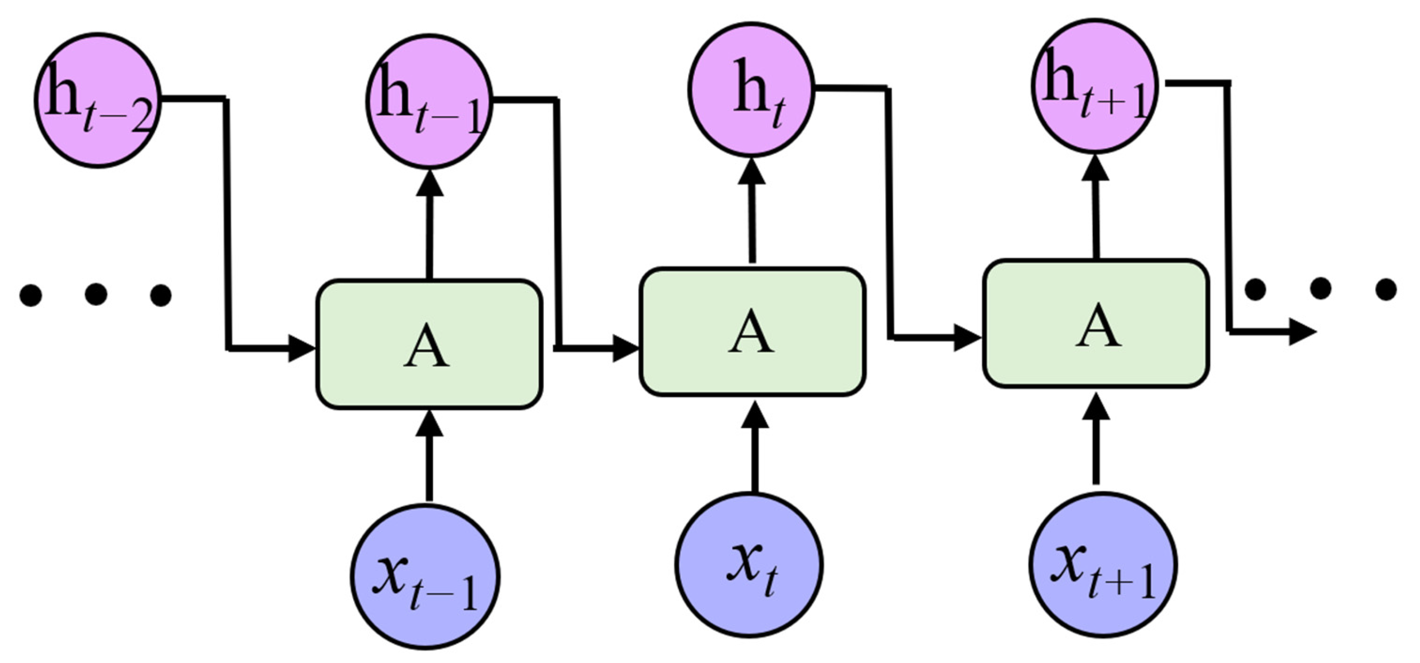
Figure 1. Schematic diagram of an RNN unit.
Applsci 13 05918 g001
Figure 2. RNN model for structural response prediction.
Applsci 13 05918 g002
Figure 3. Schematic diagram of LSTM unit.
Applsci 13 05918 g003
Figure 4. LSTM model for structural response prediction.
Applsci 13 05918 g004
Figure 5. Process of solving structural response.
Applsci 13 05918 g005
Figure 6. Spectral characteristics of selected seismic acceleration records.
Applsci 13 05918 g006
Figure 7. Cluster centers of original acceleration records.
Applsci 13 05918 g007
Figure 8. Loss curves of the RNN and LSTM models in the training process (for the linear structure). (a) RNN model; (b) LSTM model.
Applsci 13 05918 g008
Figure 9. Loss curves of RNN and LSTM models in the training process (for the nonlinear structure). (a) RNN model; (b) LSTM model.
Applsci 13 05918 g009
Figure 10. PDF of prediction results by RNN and LSTM models for linear systems. (a) RNN model; (b) LSTM model.
Applsci 13 05918 g010
Figure 11. Comparison of numerical results and prediction results (RNN model for linear systems; the third layer responds [ u s 3 , u ˙ s 3 , u ¨ s 3 ] ). (a) u s 3 under the action of the seismic wave in cluster 1. (b) u ˙ s 3 under the action of the seismic wave in cluster 1. (c) u ¨ s 3 under the action of the seismic wave in cluster 1. (d) u s 3 under the action of the seismic wave in cluster 2. (e) u ˙ s 3 under the action of the seismic wave in cluster 2. (f) u ¨ s 3 under the action of the seismic wave in cluster 2. (g) u s 3 under the action of the seismic wave in cluster 3. (h) u ˙ s 3 under the action of the seismic wave in cluster 3. (i) u ¨ s 3 under the action of the seismic wave in cluster 3.
Applsci 13 05918 g011
Figure 12. Comparison of numerical results and prediction results (LSTM model for linear systems, the third layer responds [ u s 3 , u ˙ s 3 , u ¨ s 3 ] ). (a) u s 3 under the action of the seismic wave in cluster 1. (b) u ˙ s 3 under the action of the seismic wave in cluster 1. (c) u ¨ s 3 under the action of the seismic wave in cluster 1. (d) u s 3 under the action of the seismic wave in cluster 2. (e) u ˙ s 3 under the action of the seismic wave in cluster 2. (f) u ¨ s 3 under the action of the seismic wave in cluster 2. (g) u s 3 under the action of the seismic wave in cluster 3. (h) u ˙ s 3 under the action of the seismic wave in cluster 3. (i) u ¨ s 3 under the action of the seismic wave in cluster 3.
Applsci 13 05918 g012
Figure 13. PDF of prediction results of the RNN and LSTM models for nonlinear systems. (a) RNN model; (b) LSTM model.
Applsci 13 05918 g013
Figure 14. Comparison of the numerical results and prediction results (RNN model for a nonlinear system, [ u s 6 , u b ] ). (a) u s 6 under the action of the seismic wave in cluster 1. (b) u s 6 under the action of the seismic wave in cluster 2. (c) u s 6 under the action of the seismic wave in cluster 3. (d) u b under the action of the seismic wave in cluster 1. (e) u b under the action of the seismic wave in cluster 2. (f) u b under the action of the seismic wave in cluster 3.
Applsci 13 05918 g014
Figure 15. Comparison of the numerical results and prediction results (LSTM model for nonlinear system, [ u ¨ d , u b , u ˙ s 6 ] ). (a) u ¨ d under the action of the seismic wave in cluster 1. (b) u b under the action of the seismic wave in cluster 1. (c) u ˙ s 6 under the action of the seismic wave in cluster 1. (d) u ¨ d under the action of the seismic wave in cluster 2. (e) u b under the action of the seismic wave in cluster 2. (f) u ˙ s 6 under the action of the seismic wave in cluster 2. (g) u ¨ d under the action of the seismic wave in cluster 3. (h) u b under the action of the seismic wave in cluster 3. (i) u ˙ s 6 under the action of the seismic wave in cluster 3.
Applsci 13 05918 g015
Table 1. Structural response analysis methods.
MethodTypical MethodAdvantages/DisadvantagesReferences
Seismic testingShaking table loading
Seismic simulator
Reliable results, intuitive phenomena/High costs, high equipment requirements, limited test conditions[11,12,13]
Theoretical analysisResponse spectrum method
Push-over method
Energy method
Simple calculation, low computing costs, stable analysis results/Cannot reflect the dynamic characteristics, limited range of application, poor accuracy[14,15,16]
Numerical analysisFinite element method
Finite difference method
Finite volume method
Providing a wider range of structural data, wide range of application/Complex analysis process, high computational cost, high requirements for computing equipment[17,18,19,20]
Table 2. Detailed parameters of the structure.
Floor NumberStory Height (m)Mass (103 kg)Stiffness (MN/m)
13.55601508
23.55521487
33.55501482
43.55481462
53.55461432
63.55391357
Table 3. Detailed parameters of the nonlinear component.
Mass (103 kg)Stiffness (MN/m)Damping
mb61317.141.63 × 106 N·s/m
md135051.43c1 = 2.13 × 10⁷ N·(s/m)2
c2 = 1.07 × 10⁷ N·(s/m)1.75
Table 4. Input and output variables of each model.
ModelStateVariable
RNN/LSTM model for linear structureInput a ¨ g = [ a ¨ g 1 , a ¨ g 2 , a ¨ g 3 , , a ¨ g n ]
Output u s i = [ u s i 1 , u s i 2 , u s i 3 , , u s i n ] i = 1 , 2 , 3 , 4 , 5 , 6
u ˙ s i = [ u ˙ s i 1 , u ˙ s i 2 , u ˙ s i 3 , , u ˙ s i n ] i = 1 , 2 , 3 , 4 , 5 , 6
u ¨ s i = [ u ¨ s i 1 , u ¨ s i 2 , u ¨ s i 3 , , u ¨ s i n ] i = 1 , 2 , 3 , 4 , 5 , 6
RNN/LSTM model for nonlinear structureInput a ¨ g = [ a ¨ g 1 , a ¨ g 2 , a ¨ g 3 , , a ¨ g n ]
Output u i = [ u i 1 , u i 2 , u i 3 , , u i n ] i = s 6 , b , d
u ˙ i = [ u ˙ i 1 , u ˙ i 2 , u ˙ i 3 , , u ˙ i n ] i = s 6 , b , d
u ¨ i = [ u ¨ i 1 , u ¨ i 2 , u ¨ i 3 , , u ¨ i n ] i = s 6 , b , d
Table 5. Configuration of platform for model training.
ConfigurationPerformance Indicators
SystemWindows 10 64-bit
CPUIntel® Core™ i7-10875H 2.35 GHz
GPUNVIDIA GeForce RTX 2060 Max-Q 6GB
RAM64 G
Python3.8.5
Tensorflow1.6.0
Table 6. Hyper parameters of the RNN model for the linear structure.
Hyper ParameterValueHyper ParameterValue
Neurons in the hidden layer128Forgetting rate0
Number of fully connected layer1RegularizationL2 Regularization
Number of RNN layers2Learning rate0.001
Number of iterations500OptimizerAdam [39]
Minimum batch size1
Table 7. Hyper parameters of the LSTM model for the linear structure.
Hyper ParameterValueHyper ParameterValue
Neurons in the hidden layer100Forgetting rate0.06
Number of fully connected layer1Gradient threshold0.1
Number of LSTM layers2Learning rate0.01
Number of iterations500RegularizationL2 Regularization
Minimum batch size2OptimizerAdam [39]
Table 8. Hyper parameters of the RNN model for the nonlinear structure.
Hyper ParameterValueHyper ParameterValue
Neurons in the hidden layer128Forgetting rate0
Number of fully connected layer1RegularizationL2 Regularization
Number of RNN layers2Learning rate0.001
Number of iterations500OptimizerAdam [39]
Minimum batch size1
Table 9. Hyper parameters of the LSTM model for the nonlinear structure.
Hyper ParameterValueHyper ParameterValue
Neurons in the hidden layer100Forgetting rate0.06
Number of fully connected layer1Gradient threshold0.1
Number of LSTM layers2RegularizationL2 Regularization
Number of iterations500Learning rate0.01
Minimum batch size2OptimizerAdam [39]
Table 10. Error values of the RNN and LSTM models for the linear structure.
ModelIndexVariable123456
RNNEWMAPE
(%)
u 4.3881.0672.5664.0302.4531.678
u ˙ 3.0786.0893.0765.0786.0694.076
u ¨ 3.7794.6993.3656.7674.1783.001
EPEAK
(%)
u 4.5322.5843.3994.5932.4632.884
u ˙ 3.5985.6653.8555.7766.9526.287
u ¨ 4.7937.9988.5892.3885.1109.300
LSTMEWMAPE
(%)
u 2.1532.4502.7792.1093.9184.022
u ˙ 2.0312.1362.4342.5394.3464.578
u ¨ 1.1251.9242.5862.3923.0793.481
EPEAK
(%)
u 1.4401.6252.3022.9782.4321.595
u ˙ 3.7064.7536.3484.2243.8912.294
u ¨ 2.3452.3992.3582.5872.4441.989
Table 11. Error values of the RNN model for the nonlinear structure.
Indexus6ubud
Cluster 1EWMAPE (%)12.6907.00816.905
EPEAK (%)32.36642.87751.623
Cluster 2EWMAPE (%)17.91313.92325.308
EPEAK (%)21.60758.18266.567
Cluster 3EWMAPE (%)10.1029.29820.117
EPEAK (%)38.39749.99353.695
Table 12. Error values of the LSTM model for the nonlinear structure.
Index u ˙ d u ¨ d u b u ˙ b u s 6 u ¨ s 6
Cluster 1EWMAPE (%)7.1104.2746.3774.4809.13210.366
EPEAK (%)6.45617.9493.75010.62517.97831.579
Cluster 2EWMAPE (%)15.23813.7736.12910.3229.39214.566
EPEAK (%)2.34328.6962.14420.2369.05320.556
Cluster 3EWMAPE (%)7.3884.4443.0317.6985.2347.893
EPEAK (%)8.77218.4211.99338.88922.1437.826
Disclaimer/Publisher’s Note: The statements, opinions and data contained in all publications are solely those of the individual author(s) and contributor(s) and not of MDPI and/or the editor(s). MDPI and/or the editor(s) disclaim responsibility for any injury to people or property resulting from any ideas, methods, instructions or products referred to in the content.