Differential Evolution and Fuzzy-Logic-Based Predictive Algorithm for V2G Charging Stations

Abstract

This work proposes a differential evolution algorithm to control a vehicle-to-grid (V2G) system based on photovoltaic generation and energy cost curves, and constraints associated with the power converters’ operation, battery charging strategy, and initial budgets. The algorithm is designed to trade off the batteries’ state of charge and the profits gained from selling energy to the grid. To achieve this balance, a fuzzy controller is employed and acts based on forecasts of the photovoltaic generation and the cost of electricity, within prediction windows of 120 min, adapting the batteries’ rate of charging or discharging. Simulation results show that for different curves and different initial budgets, the target state of charge is reached at the end of the time horizon. By evaluating the proposed scheme under different scenarios, the algorithm’s performance is proven to be suitable for future practical deployment.

1. Introduction

In recent years, there has been a growing use of distributed generators across the electrical grid. Most of the distributed generation is supplied by alternative and renewable energy sources whose energy production is conditioned on the availability of natural resources, observing climatic conditions, and timely and seasonal cycles [1]. In this regard, frequent studies have been conducted to analyze the stability of the system and the technical impacts that may arise or need to be minimized with the insertion of new generators [2].

In this context, the concept of smart grids presents itself as a viable possibility to provide regulatory agents with the necessary data for intelligent decision-making, resulting in less vulnerability from the generator side and an encouragement for new technically viable connections. On the other hand, the popularization of electric vehicles has brought to light the need for studies evaluating the impact on the grid from the increase of these loads [3,4,5]. According to the International Energy Agency, it is estimated that the electric vehicle market has worldwide projections of reaching 22 million electric vehicles in 2030 [6]. Hand in hand with the energy demand, there are difficulties in identifying appropriate times for recharging, considering the available power capacity and the electricity cost. In addition, the possibility of vehicles acting as generators has also been widely discussed, especially in the sense of relieving the electrical system at times of peak demand, when overload issues may occur [7,8,9]. Clearly, the decision of charging or discharging becomes an optimization problem, whose instantaneous solution depends on technical, financial, and environmental factors.

Reasonable energy management is a key factor to reduce the impacts on the electrical grid. Recent studies presented strategies and optimization techniques that improved voltage regulation, losses, recharge time, storage quality, and profitability. In [10], for the electric vehicle to work with a bidirectional power flow, an energy management system was proposed by exploiting a linear programming method. The vehicle was considered as a bank of batteries whose charging and discharging were carried out to maximize the consumption of the photovoltaic energy produced in situ.

In [11], the authors analyzed several strategies and proposed a solution considering each autonomous consumer connected to a microgrid, which, in turn, was integrated into an alternating bus current that shared a connection with other local microgrids. Both microgeneration and electric vehicles were connected to the local microgrid. In [12], the proposed vehicle-to-grid (V2G) control led to a rapid and effective response to ensure the grid frequency stability, while the smart charging control satisfied the scheduled charging by the vehicle user. However, there remain research subjects on the efficiency of the proposed V2G control, impact to the battery life, secure interconnection method to the grid, and so on.

In [13], a fuzzy algorithm was proposed that worked alongside a virtual synchronous generator for different scenarios throughout the day. In that study, the main objective was to flatten the demand curve and achieve a greater equity in battery charging time. In [14], two fuzzy algorithms were presented in comparison with several optimization techniques; they showed satisfactory results, performing relatively close to an optimization metaheuristic technique, with less computational complexity and the introduction of expert knowledge into the model.

In [15], two charging algorithms based on a self-critical logic were presented. The first one sought optimal results regardless of the computational cost and high storage requirements. The second sought a computational optimization to make data processing faster; however, it sacrificed performance when solving the optimal charging cost. In [16], a hybrid electric vehicle was considered, and an evolutionary algorithm was proposed capable of making short-term predictions for charging and discharging, resulting in a greater autonomy and fuel economy. Ref. [17] presented a two-step algorithm, working both with the grid information and with information from the client itself. Although the results were satisfactory, the authors made it clear that the interaction of the grid with the batteries needed further improvement so that the charging and discharging could be better planned.

In [18], a new approach was taken, which prepared the system so that it could offer to the users of the charging station different charging speeds, presenting them the possibility of utilizing the V2G technology, developed for obtaining data and testing its robustness. After the energy flow in the system occurred, the overall system was priced based on the resulting energy exchanged between the vehicle and the grid.

Finally, the papers [19,20,21] had a similar focus, analyzing the energy flow in the distribution grid, with multiple charging strategies adopted, which were developed with smart algorithms as their bases. The proposals sought to mitigate grid losses as well as to verify whether the grid could deal with multiple charging stations at the same time at multiple points. These works showed that there were many ways to approach the problems imposed by the V2G and energy management concepts, noticing its expansion around the world. It is possible to work with basic or more complex systems, with multiple vehicles connecting to the grid.

Observing the before-mentioned works and the necessity of improvements in the energy management systems of electrical charging stations, this work proposes a predictive control algorithm based on the differential evolution method, utilizing generation and cost data as inputs for a fuzzy controller. The algorithm coordinated with a fuzzy logic aims to optimize the charging of the batteries of an electric vehicle connected to a charging station with its local generation and connected to the grid. The V2G concept is exploited, allowing the electric vehicle to charge itself and to feed electricity back into the grid to supply demands. The process optimization was conceived to reduce the cost of charging, prioritizing periods when the energy produced is sufficient to carry out the charging or when the energy cost purchased from the grid is as low as possible. The optimization also seeks to sell the stored energy to the electricity grid at a time when energy demand is high, optimizing the financial performance and ensuring a state of charge greater than 50%.

The main novelty of this work lies in the utilization of two inputs to run the algorithm seeking a compromise between the SoC of the vehicle battery and the profit that can be obtained by selling energy from the battery to the grid. This approach guarantees a greater flexibility of the cost function, automatically adapting it to the scenario at hand and, finally, achieving a better operation in a range of different situations.

The remaining of the manuscript is organized as follows: in Section 2, the optimization algorithm is described whereas in Section 3, the results under different profiles of photovoltaic generation and energy costs are presented and subsequently discussed in Section 4. Section 5 concludes the manuscript by summarizing the main features of the proposed algorithm.

2. Materials and Methods

As presented in Figure 1, the considered V2G system is composed of multiple converters, both DC–DC and DC–AC. The proposed algorithm consists of a differential evolution component, featuring a 2-hour receding-horizon time window, and a fuzzy logic component that adapts certain parameters online to attain better performance. The final goal of the algorithm is to determine each converter power flow as ultimately specified by their currents. To operate the V2G system optimally, forecasts of the solar irradiance and the energy tariff are exploited, both being fully time-varying, which adds to the complexity of the overall task.

2.1. Decision Variables and Constraints

The current flowing from the photovoltaic array is denoted by $I_{PVt}$, where “t” identifies the minutes within the prediction horizon of 2 h. This index also depends on the variable “z”, which identifies the absolute time at which the algorithm is. At the beginning of the day, for example, “$z=1$” is adopted and is updated at each algorithm run, in order for it to be applied to a full day or any period of time that is required. The variable ${\beta }_t$ represents the energy cost. $I_{bi}$ is the instantaneous charging current of the battery bank whose charging and discharging limits obey (1). $K_2$ is the maximum charging current value. $-K_2$ is related to the maximum discharging, and current “i” is the battery charging current.

The prediction control algorithm used is based on the receding horizon strategy [22], which consists in the horizon being rolled forward as the optimization algorithm is solved. As an example, the first two hours of the cost and photovoltaic curves are utilized to run the algorithm, utilizing t as the index. At the end of the algorithm’s first run, t is reset and the calculated currents are used for the system operation in the first minute. Then, z is incremented and a new prediction window of 2 h is used by employing the second minute as the initial one.

It is important to highlight that the battery charging limits do not necessarily have the same values, as they can be defined based on the battery type and user restrictions. Current $I_{git}$, as observed in (2), corresponds to the portion that flows into the grid or is absorbed from it based on the charging current that was initially generated. The limits set for $I_{git}$, identified in (3) as $K_5$, are related to the power of the bidirectional converter that interfaces the system and the grid. According to Figure 1, it is relevant to state that positive values for $I_g$ correspond to the current flow from the grid to the electrical charging station.

$$-K_2\le I_{bi}\le K_2$$

(1)

$$I_{git}=I_{bi}-I_{PVt}$$

(2)

$$-K_5\le I_{git}\le K_5$$

(3)

2.2. The Optimization Algorithm

To run the algorithm, it is necessary to generate an initial population, namely, $Po{p}_1$. It is composed of individuals who essentially represent the current $I_b$. Despite being a randomly generated population, each individual that composes it must respect the restrictions imposed by (1) and (3). Therefore, according to the flowchart presented in Figure 2, for every generated individual, after constraint (1) is met and using the photovoltaic (PV) generation data, one may find $I_g$. In turn, $I_g$ must obey restriction (3).

Additionally, other important restrictions must be considered. First, it is important to point out that a time interval of 120 min was defined to evaluate the obtained currents. This value was chosen assuming that it represented a good prediction range for $I_{PV}$ and $\beta$ in practical applications. That is, according to (4) and (5), each generated individual must be evaluated in this time interval to guarantee that the pre-established budget ($\mu$) is not exceeded and that, according to (6), the batteries’ state of charge (${\theta }_i$) does not reach physically impossible values, a restriction imposed by (7). It is valid to inform that in (6), $K_1$ encodes the battery capacity, a fundamental quantity to convert the current that flows to the battery into the state of charge. $K_1$ is adjusted according to the capacity of the bank under analysis.

$$\sum _{t=z}^{119+z}\left(I_{git}\times {\beta }_t\right)=cos{t}_i$$

(4)

$$cos{t}_i\le \mu$$

(5)

$${\theta }_i={\theta }_{i-1}+K_1\times I_{bi}$$

(6)

$$0\le {\theta }_i\le 100$$

(7)

Once all restrictions have been met, the evaluated individual is considered able to be part of $Po{p}_1$. The cost function (8), associated with each individual of $Po{p}_1$, depends on the costs associated with the consumed energy $\left(I_{git}\times {\beta }_t\right)$, the costs associated with the photovoltaic generation ($I_{PVt}$), and the remaining energy in the battery bank $\left({\theta }_i-100\right)$. The $K_3$ value depends on the energy tariff and the fixed and variable costs associated with the PV modules and equipment used in the photovoltaic generation. For a self-sustained electric charging station, disregarding the fixed implementation costs and considering that the maintenance costs are very low, $K_3$ can be considered zero. On the other hand, $K_4$ has a crucial role in (8). The value chosen for this constant defines the priority of charging the batteries over selling the stored energy. For this reason, simulations on the influence of $K_4$ were performed, and an expert system was designed to dynamically adapt this constant. Therefore, the priority of charging the battery bank was defined based on the cost of electricity and the photovoltaic energy availability.

$$F{c}_{target}=K_4{\left({\theta }_i-100\right)}^2+\sum _{t=z}^{119+z}\left(I_{git}\times {\beta }_t+I_{PVt}\times K_3\right)$$

(8)

As per the differential evolution (DE) algorithm, the initial population is improved genetically at every iteration [23]. To be effective, the usage of this evolutionary algorithm must rely on randomness of the genetic modifications. Since each individual in the population had a single feature to be updated, the crossover and mutation phases were integrated into a single step. Therefore, the crossover constant “$cr$”, with a value between 0 and 1, was compared to a random number ($rand$) also between 0 and 1. The larger the “$cr$”, the greater the chance of crossover.

The target individual ($In{d}_{target}$) is the one that will potentially be replaced by a new individual, called the test individual ($In{d}_{test}$). It is important to mention that all individuals in the population, one by one, will be targeted at some point. On the other hand, $In{d}_{test}$ will exist in case $rand\le cr$. To create $In{d}_{test}$, three random individuals from $Po{p}_1$ ($In{d}_x,In{d}_y,In{d}_z$), different from $In{d}_{target}$, are selected, and the crossover occurs following (9), $F \in \left[0,2\right]$ being known as the mutation factor [23].

$$In{d}_{test}=In{d}_x+F\left(In{d}_y-In{d}_z\right)$$

(9)

After the crossover and mutation step, it is necessary to assess whether the new individual meets the restrictions presented in (1) to (7). If $In{d}_{test}$ does not pass the existing restrictions, it is no longer evaluated and $In{d}_{target}$ keeps its value and its position in the new population ($Po{p}_{new}$). However, if $In{d}_{test}$ passes the constraints, it can be evaluated by the cost function (8), resulting in the value $f{c}_{test}$. If $f{c}_{test}$ is lower than the cost function of the target individual ($f{c}_{target}$), $In{d}_{test}$ replaces $In{d}_{target}$ into the new population. If $f{c}_{test}$ is greater than $f{c}_{target}$, it means that the new individual does not fit; thus, $In{d}_{target}$ keeps its value and position in ($Po{p}_{new}$). Finally, after the first generation, when all individuals of $Po{p}_1$ have become targets and have been evaluated, $Po{p}_{new}$ is composed of the combination of the individuals initially generated and those best adapted, generated by the DE approach.

For the next generation, $Po{p}_{new}$ assumes the position of $Po{p}_1$ and the process restarts. Since the process is iterative, always restarting for a new generation, the number of generations or the convergence of the results can be used as stopping criteria. For the prediction of the photovoltaic generation and costs, at the end of the generations, the resulting individuals correspond to the optimal value of $I_b$ for the first minute, taking into account the predicted curve for the next 119 min, which means an interval of 120 min or 2 h.

The initial photovoltaic production and cost curves are predictions of behavior. It is important to mention that in a real application, these curves are dynamic, and their profiles are updated throughout the day. Therefore, the effectiveness of the algorithm is based on the actual measurement of each minute of the day, based on the forecast for the next 119 min. That is, for each one-minute step, the input curves are updated, and the optimal current is calculated having $I_{PV}$ and $\beta$ as predicted inputs for the next two hours. In this way, the optimal operating profiles, including $I_b$, $I_g$ and $\theta$, are obtained, minute by minute, for a 24 h time interval.

3. Results

To validate the proposed algorithm, two photovoltaic scenarios were considered as shown in Figure 3. These are directly expressed in terms of the available current $I_{pv}$. The blue curve, referred to as “sunny”, represents a typical sunny day with few clouds and a high overall energy availability. The red curve, referred to as “cloudy”, represents a day with intermittent rains and a greater number of clouds.

The time-varying energy tariff employed in this study is shown in Figure 4, displaying the usual peaks at around noon and in the early evening due to the high demand in these periods. The latter peak is seen to correspond to a cost 67% higher than the base price of USD $0.30$.

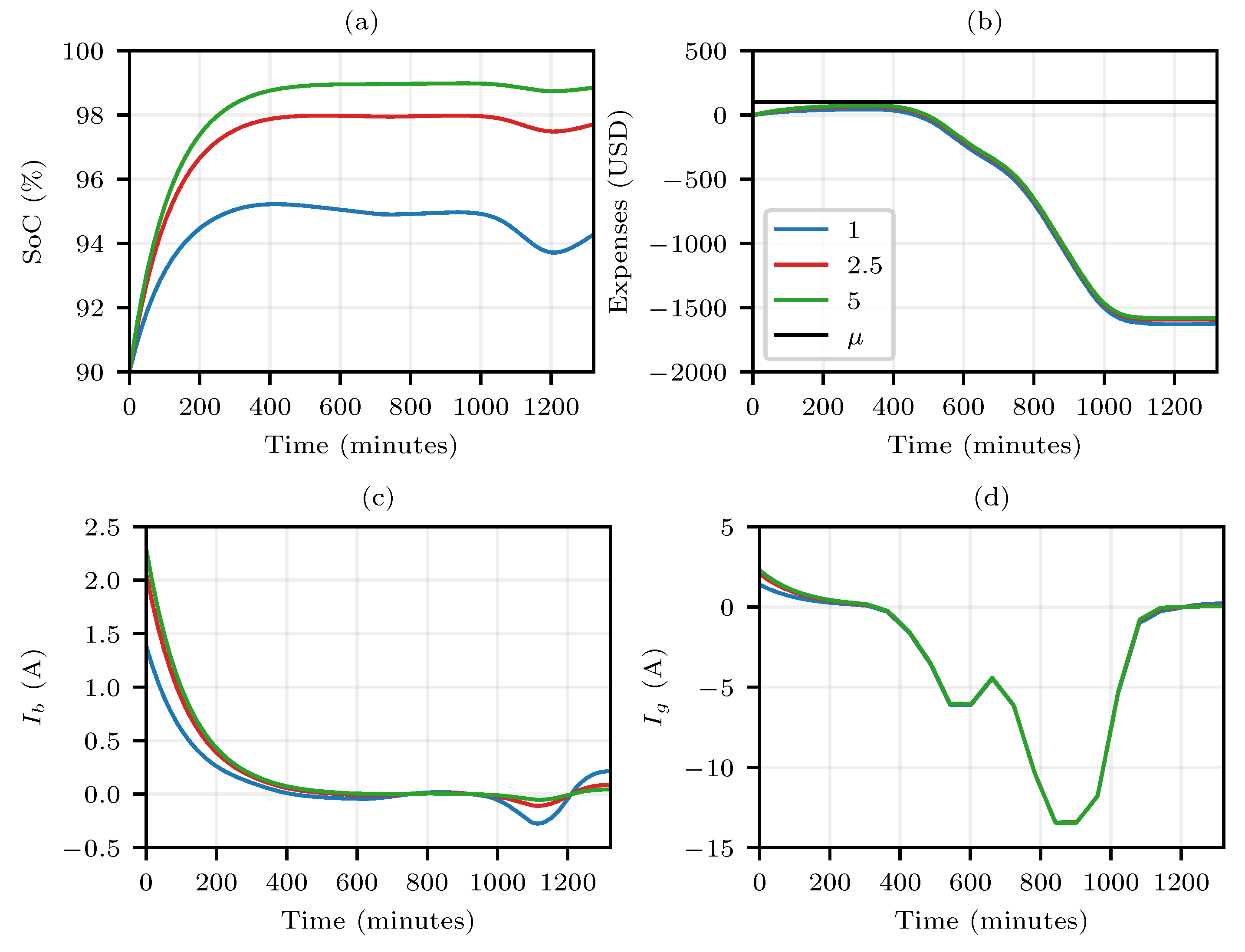
From the established scenarios, the first tests were performed to analyze the behavior of the algorithm for different values of “$K_4$”. It is worth mentioning that these tests were carried out to observe how “$K_4$” could prioritize or not the state of charge of the battery bank, directly influencing the profit achieved throughout the day, the current that flowed to the batteries, and the current that flowed to the grid. In Figure 5, it is possible to analyze the behavior of the algorithm for the “sunny” curve, assuming values between zero and one for this constraint. For values of “$K_4$” greater than one, the behavior of the variables under study can be seen in Figure 6.

In Figure 5 and Figure 6, (a) shows the state of charge of the battery; (b) the profit obtained throughout the day with the purchase or sale of electricity, with positive quantities corresponding to expenses; (c) shows the current flowing to the battery, where positive values indicate battery charging; (d) presents the mains current, where positive values indicate a current flow from the mains to the batteries.

The results show that the lower the value observed for “$K_4$”, the greater the effort of the system to sell the energy stored in the battery banks. As can be seen in Figure 5c, as “$K_4$” approached zero, the time during which the discharging current in the battery is maximum increased. In Figure 5a, for each value of “$K_4$”, it is possible to see the speed at which the battery state of charge decayed, as well as the balance point between purchased and stored energy. As an example, assuming “$K_4$” equaled 0.1, the algorithm sought to maintain the state of charge at approximately 50% (Figure 5a). As shown in Figure 5d, this balance led to the situation in which all the energy generated at the electric charge station was sent to the grid, which produced profits throughout the day (Figure 5b).

Something interesting to observe is that, at the end of the day, for the condition of “$K_4=0.1$”, the batteries were activated to send energy to the grid in an interesting moment considering the energy price; however, soon after, they drain some current from the grid to maintain the previous state of charge. This may also be associated with the fact that the peak of energy cost matched the moment when the photovoltaic generation rapidly decayed.

On the other hand, in Figure 6, the efforts of the system to preserve the batteries charged can be observed. The value of “$K_4$” directly interfered with the final state of charge. In Figure 6a,c it is observed that the system stabilized the state of charge at 95%, 98%, and 99% for the respective values of “$K_4$” of 1, 2.5, and 5. In Figure 6b,d, it is confirmed that the system balanced quickly, allowing the energy generated throughout the day to be fully sent to the grid, keeping the batteries sufficiently charged, and maximizing profits. As in Figure 5c, it can be seen in Figure 6c that at the moment of higher costs, it became attractive for the batteries to supply current to the grid; nevertheless, they quickly recovered the equilibrium of charge after the tariff reduction.

From the initial analyses, it was possible to carry out a study in order to adapt the values of “$K_4$” so that, at the end of the day, the battery banks were in a satisfactory state of charge and so that, at the same time, the electric station generated a profit. Therefore, it was considered reasonable to set the spending ceiling at USD 100 for the first day and USD 300 for the supposed second day. This variation in the spending ceiling considered the profits added to the budget and, consequently, eliminated the limiting factor that the budget imposed on battery charging in the event of the absence of photovoltaic generation.

In sequence, we analyzed the behavior of the system parameters from the linear variation in “$K_4$” as a function of the photovoltaic generation curve. Therefore, the proposal considered valuing the charging of the batteries during maximum photovoltaic production. Another proposal consisted of linearly varying “$K_4$”, taking the cost of energy from the grid as the input variable, maximizing the charging for situations in which the cost was lower. It is important to highlight that for the proposed work, the photovoltaic generation and electricity cost profiles did not present any correlation, being completely independent. Obviously, we could not exclude the possibility that in certain places, such profiles were linearly dependent, which would rule out the need to analyze “$K_4$” for the two previous proposals.

With a view to the proposed variation of “$K_4$”, it is worth considering that when charging the batteries during peak generation, regardless of whether the batteries are charged or not, the energy surplus will naturally flow to the electrical grid. This allows, during the energy cost peak, the stored energy to be used to generate a greater profit, because depending on the form of negotiation, such energy can be dispensed to the grid in the absence of photovoltaic generation and for a more attractive price. For the proposals of a linear variation of “$K_4$” as a function of the generation and cost profiles, 0.1 and 5 were adopted as minimum and maximum values, with such limits being established, respectively, for situations in which recharging and charging had the highest priority.

Considering that the relationship of “$K_4$” with the generation and cost profiles was not necessarily linear and that, in a real scenario, the profiles’ behavior, in addition to being unpredictable, were not correlated, as a strategy to match the previous proposals, a fuzzy system was created, having as inputs the photovoltaic generation curve and the electricity cost curve and, as an output, the value of “$K_4$”. With the proposed logic, the battery was charged more than 90% at the beginning of the day, adopted as 5 AM or 6 AM.

The membership functions of the inputs and output are depicted in Figure 7. For the inputs, the strategy was to utilize the trapezoidal forms for the values that were close to the max ranges, which were selected as the minimum and maximum values of the photovoltaic and cost curves. This way, it worked as a crisp number in that region and started to operate as a fuzzy logic operator as the measures increased or decreased. The abbreviation adopted were L for low, M for medium, and H for high.

Given that the fuzzy logic has two inputs with three membership functions each, there were a total of nine rules, presented in

Table 1. Proposed fuzzy logic mapping.

INPUTS			$\mathit{\beta }$
		L	M	H
${\mathbf{I}}_{\mathbf{PV}}$	L	B	M0	S2
	M	M1	M0	S1
	H	S2	S1	S0

, contemplating each one of the possible cases. The abbreviation adopted were S for small (S0, S1 and S2), M for medium (M0 and M1) and B for big, referring to the obtained $K_4$ output.

It is important to notice that the analysis obtained in Figure 5 and Figure 6 established that the system was much more sensitive when it works with $K_4$ varying in an interval between zero and one. Thus, the output membership functions were built by focusing on the impact that lower values of $K_4$ had when applied to the system, in a way where the small functions had much more interactions and influence on each other than the medium and big functions, so that, for higher values, the controller focused on establishing an optimal state of charge.

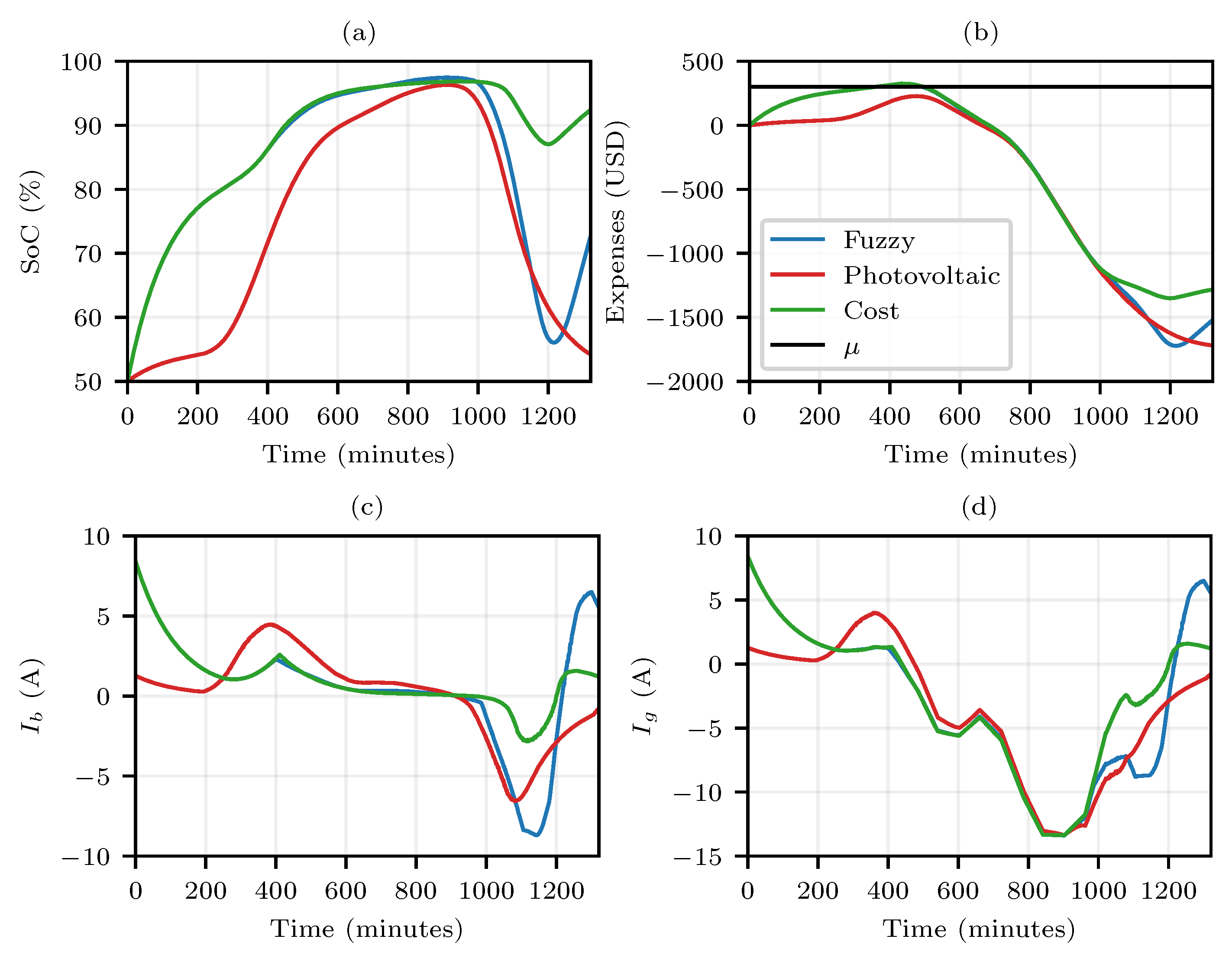
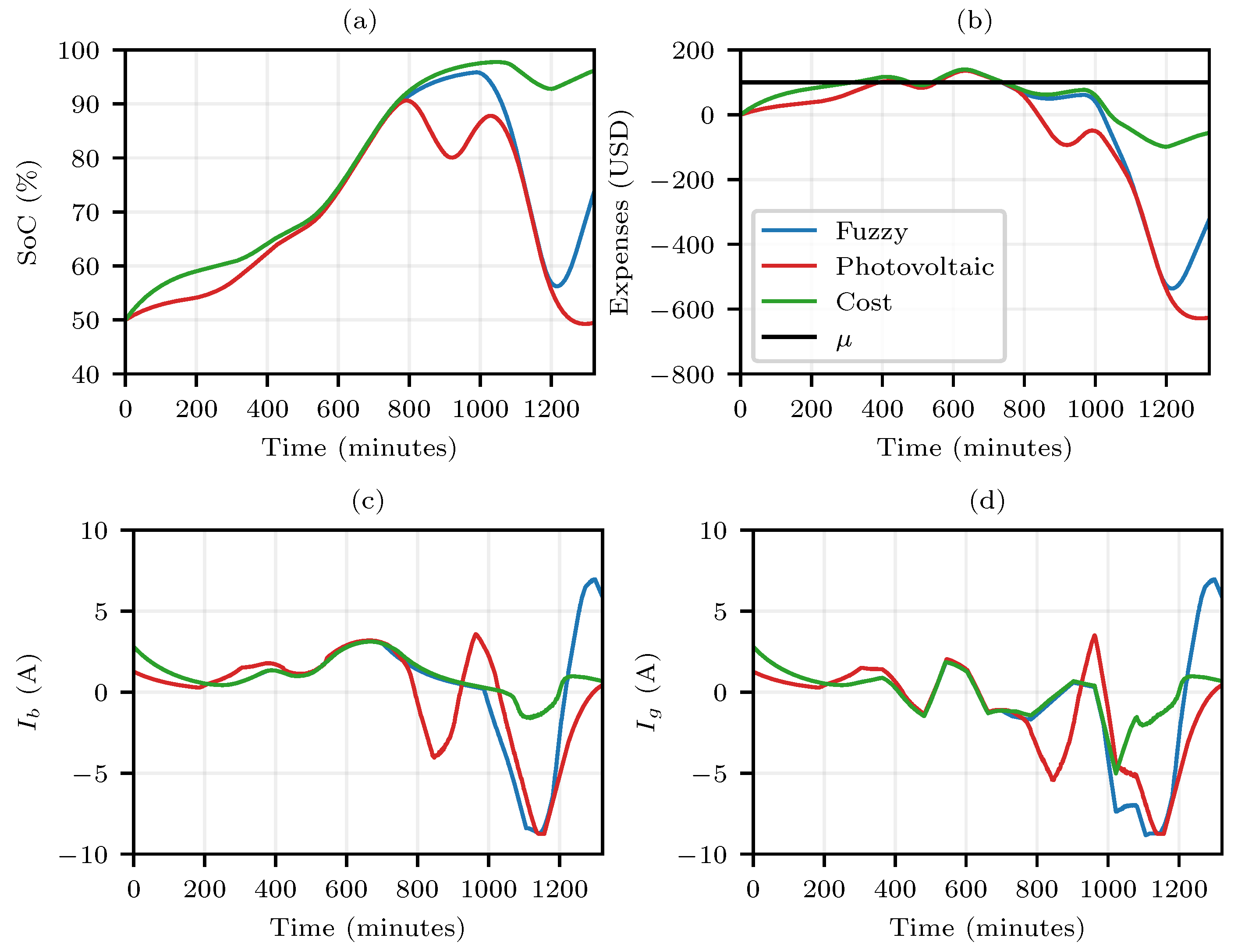
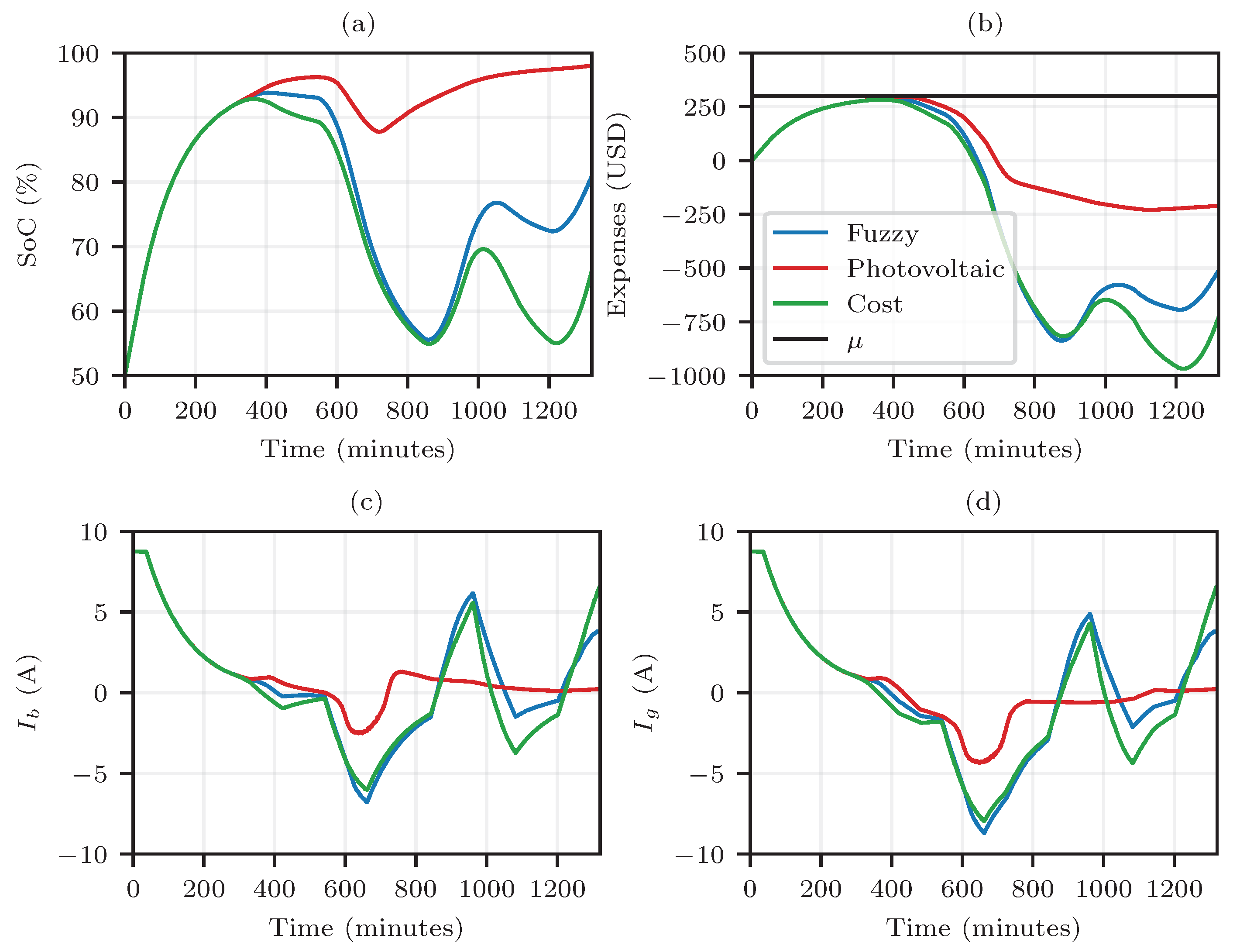
In Figure 8, Figure 9, Figure 10 and Figure 11, the curves called “Photovoltaic” correspond to the proposal that prioritized battery charging when there was greater photovoltaic generation. The so-called “Cost” curves correspond to the proposal in which the energy stored in the batteries was sold at the energy cost peak and the batteries were charged when the cost was minimal. For Figure 8 and Figure 9, the “sunny” profile of photovoltaic generation was used, while in Figure 10 and Figure 11, the “cloudy” profile was adopted.

From the analysis of Figure 8, Figure 9, Figure 10 and Figure 11, it is possible to observe that the three algorithm alternatives have similarities. It is evident that the fuzzy curve, which takes into account self-generation and electricity cost, primarily respects the cost curve during the moments of reduction in photovoltaic generation. On the other hand, for the moments when there is energy from the photovoltaic system, the Fuzzy system tends to migrate to the “Photovoltaic” curve.

The analyses showed that for both cost and fuzzy curves, depending on the available budget, the algorithm sought to increase the battery state of charge so that, at the beginning of the next day, there was a sufficient availability of stored energy. On the other hand, the photovoltaic curve showed the priority was on the battery charging when the photovoltaic generation was sufficiently high, so that, at the beginning and end of a day, the battery bank had a charge state of approximately 50%. Assuming that the battery bank was mobile (i.e., part of a vehicle), the low percentage of charge storage at the beginning of the day constituted a major disadvantage for the algorithm with the photovoltaic profile; however, if the battery bank was stationary, the behavior of the photovoltaic curve became attractive, mainly because it increased the obtained profits.

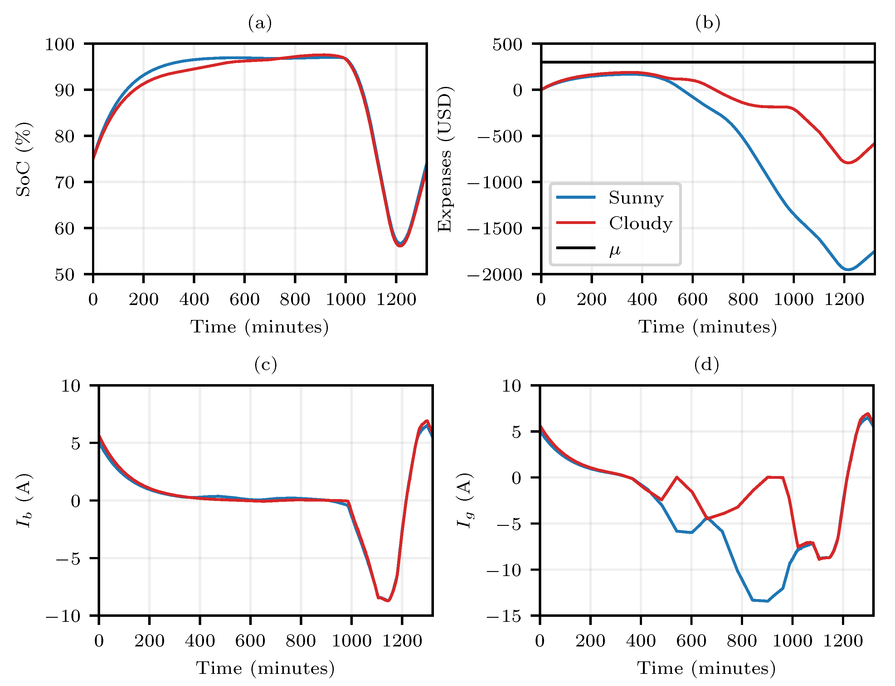
In comparison with the cloudy profile, even though the sunny profile injected a higher average current, the curves presented a very similar behavior regarding the battery charging (Figure 12a,c). From the obtained results, we obtained that between 5 a.m. and 6 a.m. (300 min and 360 min, respectively), the battery bank was in a state of charge between 90% and 95%. With adjustments in the fuzzy rules, this state of charge could also be higher, even reaching full load.

Figure 12b,d illustrate that the greatest discrepancies were seen in the injection of the generated current and the total profit at the end of the day. It is also worth mentioning that the variations in the cloudy profile did not bring as much impact to the system as the variations in the sunny profile, although the current injected into the cloudy profile is smaller.

In the last analysis, in Figure 12, the comparison of the fuzzy proposal is presented for the different generation profiles (sunny and cloudy). In that analysis, it was assumed that the initial state of charge was the value recorded at the end of the simulations shown in Figure 8, Figure 9, Figure 10 and Figure 11, in this case, about 75%.

With the purpose of validating the algorithm for different scenarios, the photovoltaic production and cost curves used in other articles were selected. In Figure 13 and Figure 14, respectively, curves similar to those shown in [17,23] are presented.

The photovoltaic curve utilized presented very small values of injected current by panels. On the other hand, the price curve exhibited steps throughout the day, instead of smooth changes as in Figure 4.

In Figure 15 and Figure 16, the resized fuzzy controller results are presented for the new curves for the budgets of USD 100 and USD 300, respectively.

Since there were only small effects caused by the panels in the cases of Figure 15 and Figure 16, it is seen that the system behavior was the same for both the photovoltaic and the cost curves in the first period for both budgets. Moreover, this was not observed in previous scenarios. Furthermore, in Figure 15a,b and Figure 16a,b, the three curves started aligned, but the fuzzy one tended to follow the cost curve behavior as time passed. One also sees that, at the end of the day, the fuzzy controller tended to value higher SoC levels.

4. Discussion

From the curves shown and discussed in the previous section, one can see that no single fixed value of $K_4$ in the cost function would deliver a reasonable performance in all scenarios. Furthermore, not even a linear relationship between any of the inputs, PV generation, or energy cost and $K_4$ would suffice. Our approach implicitly defined a nonlinear relationship that took into account both inputs, adapting $K_4$ and finally attaining a greater cost reduction throughout the day. As a result, the fuzzy logic component was central to the V2G control algorithm.

The main strength of the proposed algorithm is its generality, in that charging stations of different sizes could be tackled with it. Additionally, operational constraints associated with them could be incorporated, tailoring the algorithm to the specific V2G system at hand. Clearly, one should understand that the more constraints are imposed on the optimization model, the higher the final operational cost will be. The generality of the presented investigation aimed at exploring how the two uncertain inputs (PV generation and electric tariff) could be handled by the fuzzy logic block at a high level of abstraction, without the interference of additional low-level constraints. Yet, the interplay among all these components is regarded as being interesting and will be the focus of future work.

5. Conclusions

In this work, a specialized algorithm was proposed to operate a V2G system composed of a PV array, a battery bank belonging to an electric vehicle, and an interface with the electrical grid. The algorithm optimized the currents being drawn or injected by each component while taking into account an objective that balanced the state of charge of the batteries and the monetary cost of operation. As the system heavily depended on the PV generation values and the electricity tariff throughout the day, those two quantities impacted the optimizer. To better cope with the changing nature of these two inputs, a fuzzy logic component was developed and tested in a number of different scenarios. The results shown here corroborated the suitability of the proposed scheme to be deployed in practice on a real V2G platform, a project that is currently under development.

Directions for possible future investigations include the use of alternative methods for optimizing the cost other than the differential evolution methodology. From a practical viewpoint, the best optimizer will also clearly be a function of the available computing power in a real V2G scenario. Finally, the matter of imprecise measurements and forecasts should be investigated as these have an important influence on the overall results.