Abstract
The purpose of this study was to enhance the accuracy of the calorific value estimation of coal by applying data preprocessing methods in laser-induced breakdown spectroscopy (LIBS). The Savitzky–Golay (SG)-smoothing and SG derivative preprocessing methods were adopted to improve the accuracy of the prediction model. The relationship among the original, SG-smoothing-pretreated, and SG derivative-pretreated LIBS data and their elemental concentrations were determined using the partial least squares regression (PLSR) model. In order to compare the reliability of each PLSR model, the coefficient of determination, root mean square error (RMSE), relative error, and RMSE average were used. As a result, the reliability of the PLSR model processed with the SG derivative method was the highest, and the root mean square average was the lowest among the three models. The predictability of the concentration of each element using the PLSR model pre-processed by the SG derivative was confirmed with the residual predictive deviation parameter. The predicted calorific value was estimated from the predicted concentrations of elements in coal using Dulong’s equation. The PLSR model pretreated by the SG derivative showed the lowest error compared to the calorific value of mixed coals obtained via the chemical analysis.
1. Introduction
In Korea, the amount of power generated from different sources consists of 39.6% from coal-fired power plants, 30.0% from nuclear power plants, 22.4% from liquefied natural gas combined cycle power plants, 4.2% from renewable energy sources, and 1.2% from hydroelectric power plants. Although the proportion of coal-fired power generation should be reduced due to environmental pollution-related problems, for which legislation has been in place since 2000, coal-fired power generation has accounted for a consistent, significant portion of about 40% from 2010 to 2016 [1]. To reduce the cost of electricity production, low-quality coal with low calorific value is used and mixed with various types of coal in Korea.
Coal is roughly composed of 69% carbon, 15% oxygen, 8.5% coal ash, 5% hydrogen, 1.5% nitrogen, 0.7% sulfur, and 0.3% other components. Carbon is an important component with respect to the calorific value of coal. However, nitrogen and sulfur cause environmental problems, such as air pollution. It is important to quantitatively analyze carbon, hydrogen, oxygen, and sulfur components to calculate coal’s calorific value, and the precise analysis of coal’s nitrogen and sulfur components is necessary to address environmental pollution-related problems such as air pollution.
Research on the components of coal has been actively conducted with X-ray fluorescence spectrometry (XRF), prompt gamma neutron activation analysis (PGNAA), and laser-induced breakdown spectroscopy (LIBS). XRF has the disadvantage of a long measurement time [2]. The neutron source used in PGNAA can have potentially hazardous effects on the human body [3]. In LIBS plasma is produced on the surface of a given sample for a short time via laser irradiation. A continuum spectrum occurs during the initial process of plasma formation. Consequently, light with the characteristic wavelengths of the sample’s elements is emitted, and the emitted light is collected by a spectroscope. The collected LIBS spectral data can be used for qualitative and quantitative analysis. Furthermore, it is possible to analyze these data in real time. All the elements present in the periodic table are theoretically measurable.
Due to the above advantages, studies on various materials such as coal, water, soil, thin films, and fly ash are being actively conducted using LIBS [4,5,6,7,8]. LIBS can be used to analyze volatile materials in powdered coals [9,10]. Wang et al. [11] used 24 samples of bituminous coal and measured carbon, hydrogen, and nitrogen as the main elements in coal using LIBS. The measured carbon and hydrogen components were examined using a partial least squares (PLS) model. Pei et al. [12] used partial least squares regression (PLSR) model to estimate the oxygen content in 34 coal samples by using time-of-flight secondary ion mass spectrometry. Bona et al. [13] measured the carbon, hydrogen, nitrogen, and sulfur content in coals using transmissive diffuse reflectance infrared Fourier transform and the attenuated total reflectance method. The authors determined the carbon, hydrogen, and sulfur content through a PLSR model with the root mean square error (RMSE) for calibration and cross-validation. Wang et al. [14] measured 199 samples of coal using near-infrared reflectance spectra (NIRS). These samples were divided into four groups, and the sulfur content of the coal was measured. The original data without pre-processing were compared with PLSR data pre-processed by Savitzky–Golay (SG) smoothing. Li et al. [15] analyzed the calorific value of 44 coal samples using LIBS and analyzed the data with the original data and the data pre-treated with Savitzky–Golay (SG) derivative method by constructing a PLSR model.
In this study, experimental samples were made by mixing powder coals into pellets. These pellets were analyzed using LIBS. The data were pre-processed with two methods, namely, SG smoothing and the SG derivative, to produce PLSR models via multivariate analysis. To compare the reliability of the PLSR models, the coefficient of determination (R2), root mean square error (RMSE), relative error, and average RMSE were adopted as parameters. Through the above PLSR models, the concentration of each element can be predicted, and a predicted calorific value can be obtained from the concentration of each element.
2. Materials and Methods
The schematic diagram of LIBS system is presented in Figure 1. A nanosecond-pulsed Nd:YAG laser operating at a wavelength of 1064 nm is used to irradiate the sample’s surface to generate plasma. An optical fiber transmits light emitted from the plasma to a spectrometer (J200 Applied Spectra, Inc., Fremont, CA, USA). The spectrometer covers a wavelength range from 190 to 890 nm with 5 channels. The LIBS system is controlled by a computer, which also analyzes the spectral data. Pelletized samples are created by blending various powdered types of coals. A 4th-harmonic Nd: YAG laser was used for irradiation, which employed a 30 mJ/pulse and operated at 1 Hz at a wavelength of 1064 nm.
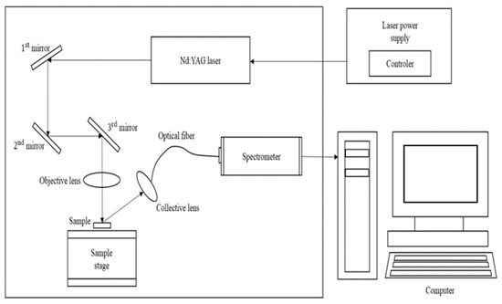
Figure 1.
Schematic diagram of the J200 LIBS measurement system.
To improve measurement accuracy, a total of 49 spots are irradiated in a 7 × 7 pattern on the sample’s surface, as shown in Figure 2. The atoms and ions are excited to a high energy level after a certain period of time and then return to the ground state. In the initial stage, continuous spectra with small intensities appear, and the peak emission lines are produced after a few microseconds. It is important to set an appropriate delay time when collecting signals by a spectrometer after laser pulse irradiation. If the delay time is set to be too long, the plasma will cool down and the peak emission lines will not be distinguishable [16]. In this study, in order to obtain the best signal to background ratio, a gate delay time and a repetition rate were chosen as 1.4 μs with 1 Hz detection.
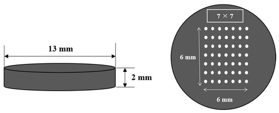
Figure 2.
Mixed coal sample pellet.
Ten coal samples imported from Indonesia, Australia, etc., were used: MSJ-1, MSJ-2, Gunvor, Peabody, Noble, Lanna Harita, Whitehaven, MacQuarie, Glencore, and Carbo One. To produce blended coal samples in a pellet form, 2 of the 10 coal samples were selected, their weights were adjusted to 0.3 g with various mixing ratios, and they were then pressed using a pelletizing machine (PN 181-1110) with a hydraulic press. Pellets with a 13 mm diameter and 2 mm thickness were produced by applying 10 tons of force. The concentration ranged from 65.75 to 74.1% for carbon, from 4.69 to 5.26% for hydrogen, from 8.96 to 18.02% for oxygen, and from 0.52 to 1.44% for sulfur. The calorific values lay between 6360 and 7275 kcal/kg. The concentration and calorific value of each coal sample were analyzed at Daeduck Analytical Research Institute for carbon, hydrogen (using the 5E Series C/H/N elemental analyzer), and sulfur (using the 5E-S3200 Coulomb sulfur analyzer). The oxygen concentration was calculated by subtracting the concentration of the remaining elements and the concentration of ash from 100%. The calorific value was determined by the 5E-C5508 automatic calorimeter. The precision accuracy was 200 ppm.
Unscrambler X version 10.3 (CAMO) software was used to evaluate the concentration and calorific value of each element in mixed coals. The PLSR model is known as a form of PLS2 method [17].
In this study, the concentration and calorific value of each element of mixed coals were used as reference values, which constitute the response variable Y of the PLSR model, and the measured LIBS spectrum data were used as the prediction value. In most cases a data-processing method is adopted for the data obtained from LIBS, but in other spectroscopic methods, such as near-infrared spectroscopy, are employed alongside to perform qualitative and quantitative content analysis.
The first spectrum data obtained through LIBS are called the original data, and the original data obtained via PLSR models are compared with the data obtained via pre-processing. The data pre-processing methods used were the SG-smoothing method and the SG derivative method. The SG-smoothing method reduces random noise and removes information that is not clearly useful. It is important to properly select the polynomial order and number of smoothing points to use this method. The SG derivative method uses the SG algorithm and extracts relevant information but increases noise. In the SG derivative method, the spectra are derived to reduce interference from spectral lines, separate overlapping peaks, and improve resolution.
3. Results and Discussion
3.1. Mixed Coal Major Elements Analysis
Figure 3 shows the entire set of the LIBS spectra of the four mixed coal samples’ carbon peaks at 193 and 247 nm. With different concentrations, they show distinguished spectral characteristics. The characteristic wavelengths of carbon, hydrogen, oxygen, and sulfur are 247.856, 656.286, 777.421, and 416.247 nm, respectively. Due to the minute fraction of sulfur, its peaks are not clearly noticeable. However, the characteristic peaks for carbon, hydrogen, and oxygen are clearly distinguished. In the case of the peak at 193 nm, the intensity is relatively small. However, the intensity at 247 nm is large enough to be clearly distinguished. Therefore, 247 nm was selected for this study, and statistical analysis was performed.
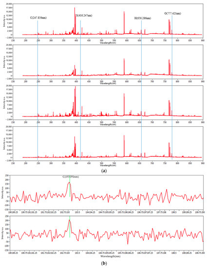
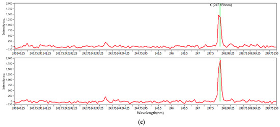
Figure 3.
(a) LIBS spectra of mixed coal samples and carbon peaks of mixed coal samples at (b) 193 nm and (c) 247 nm.
3.1.1. Partial Least Squares Regression (PLSR) of Major Elements of Mixed Coal
Quantitative analysis of carbon, hydrogen, oxygen, and sulfur in the mixed coal was conducted. The relationship between the concentration of major elements in the mixed coals obtained by conventional analysis and the LIBS spectrum intensity data obtained by the laser irradiation of the mixed coals was expressed using the PLSR model. In addition, the data obtained via the SG-smoothing and SG derivative data-pre-processing methods applied to the original data were used to construct a PLSR model, which was compared to the PLSR model of the unprocessed data, i.e., the original data. As a type of multivariate analysis method, the PLSR model can provide a relationship between a set of predictor variables X and a set of response variables Y.
The parameters for comparing the PLSR models were compared using the coefficient of determination, R2, and the RMSE. The R2 can be defined by the following equation:
where n, , , and are the number of samples, the sum of squares regression, the sum of total squares, and the sum of squares error, respectively. The R2 ranges from 0 to 1. As the R2 is closer to 1, the model’s reliability is considered to be higher.
In this study, the root mean square error of calibration (RMSEC) and the root mean square error of cross-validation (RMSECV) were employed as the testing parameters for investigating the performance of PLSR. The RMSEC and RMSECV can be calculated by the following equation:
where n, , and yi are the number of samples of calibration and cross-validation, the reference concentration of the ith sample, and the predicted concentration of the ith sample, respectively. The RMSE ranges from 0 to 1. As the RMSE is closer to 0, the model’s reliability is higher.
Figure 4a shows the PLSR model of the original data for carbon. Figure 4b–d present the PLSR models that employed SG-smoothing-based pre-processing with third-order polynomials and three, five, and seven smoothing points, respectively. In Figure 4a, the R2 values for calibration and for cross-validation are 0.94279 and 0.91218, respectively. The RMSEC and RMSECV are indicated as 0.5236 and 0.65972, respectively. As shown in Figure 4b, the R2 values for calibration and cross-validation are 0.94983 and 0.92042, respectively. The RMSEC and RMSECV are indicated as 0.49035 and 0.62801, respectively. The PLSR model pre-processed with fourth-order polynomials and with 5 smoothing points is shown in Figure 4c. The R2 values for calibration and cross-validation are 0.94706 and 0.92122, respectively. The RMSEC and RMSECV are indicated as 0.5037 and 0.62483, respectively. In Figure 4d, the R2 values for calibration and cross-validation are 0.94678 and 0.92491, respectively. The RMSEC and RMSECV are indicated as 0.50503 and 0.61004, respectively. Compared to the PLSR model of the original data, the R2 for calibration and the RMSEC value are improved, as shown in Figure 4b. In Figure 4d, the R2 for cross-validation and the RMSECV values are improved.
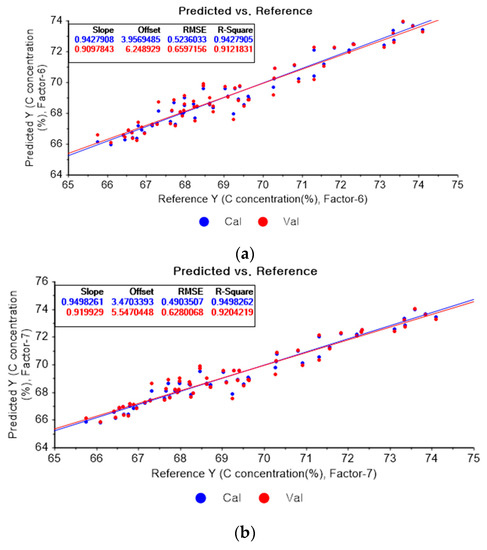
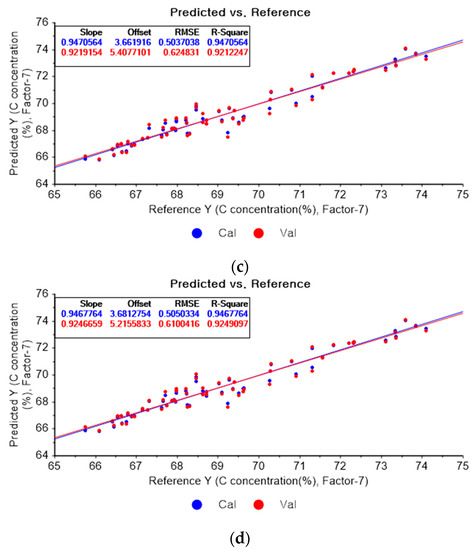
Figure 4.
PLSR model of carbon concentration with (a) original data and PLSR models pre-processed with SG smoothing by adopting (b) fourth-order polynomial with three points, (c) fourth-order polynomial with five points, and (d) fourth-order polynomial with seven points.
Figure 5a depicts the PLSR model of the original data for carbon. Figure 5b–d present the PLSR model pre-processed with the SG derivative adopting the second-order derivative and the second-order polynomials with one, three, and five smoothing points, respectively. In Figure 5a, the R2 values for calibration and cross-validation are 0.94279 and 0.91218, respectively. The RMSEC and RMSECV are indicated as 0.5236 and 0.65972, respectively. As shown in Figure 5b, the R2 values for calibration and cross-validation are 0.96101 and 0.90156, respectively. The RMSEC and RMSECV are indicated as 0.43227 and 0.69847, respectively. In Figure 5c, the R2 values for calibration and cross-validation are 0.94195 and 0.90657, respectively. The RMSEC and RMSECV are indicated as 0.52745 and 0.68047, respectively. In Figure 5d, the R2 values for calibration and cross-validation are 0.94173 and 0.90919, respectively. The RMSEC and RMSECV are indicated as 0.52845 and 0.67086, respectively. As shown in Figure 5b, the R2 values for calibration and the RMSEC values are improved compared to those from the PLSR model using the original data. However, the R2 for cross-validation and the RMSECV are lower. The R2 values for calibration and RMSEC are the closet to 1 in the PLSR model pre-processed with the SG derivate.
Figure 5.
PLSR model of carbon concentration with (a) the original data and PLSR models pre-processed with SG derivative by utilizing (b) first-order derivative and third-order polynomial with five points, (c) first-order derivative and third-order polynomial with seven points, and (d) first-order derivative and third-order polynomial with nine points.
The carbon concentration can be predicted through the above-mentioned PLSR models. The measured carbon concentration and the predicted carbon concentration are shown in Figure 6. The maximum relative errors in the PLSR model employing the original data and in the PLSR model pre-processed with SG smoothing were 1.88 and 1.95%, respectively. The maximum relative error of the PLSR model employing the SG derivative was 2.15%. However, the relative average errors of the PLSR model using the original data, the PLSR model pre-processed with SG smoothing, and that pre-processed via the SG derivative are 0.59, 0.55, and 0.50%, respectively. Overall, the relative error of the PLSR model pre-processed with the SG derivative is smallest among the above-mentioned cases.
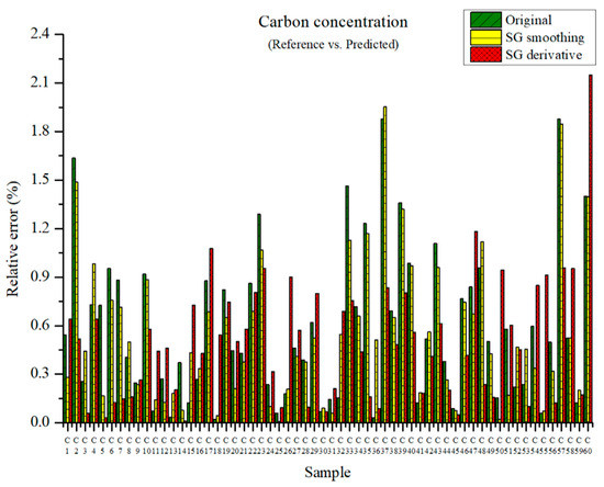
Figure 6.
Comparison of relative errors between measured and predicted carbon concentrations for the PLSR models using the original data and pre-processed data.
Figure 7a presents the PLSR model for hydrogen concentration using the original data. Figure 7b–d depict the PLSR models pre-processed by SG smoothing using first-order polynomials with one, three, and five smoothing points, respectively. In Figure 7a, the R2 of calibration, the R2 of cross-validation, the RMSEC, and the RMSECV are 0.90566, 0.77827, 0.04369, and 0.06812, respectively. As shown in Figure 7b, the R2 of calibration, the R2 of cross-validation, the RMSEC, and the RMSECV are 0.90977, 0.76406, 0.04273, and 0.07027, respectively. The PLSR model pre-processed by SG smoothing utilizing the first-order polynomial with three smoothing points is shown in Figure 7c. The R2 of calibration, the R2 of cross-validation, the RMSEC, and the RMSECV are 0.88495, 0.75905, 0.04825, and 0.07101, respectively. In Figure 7d, the R2 of calibration, the R2 of cross-validation, the RMSEC, and the RMSECV are 0.86682, 0.75215, 0.05192, and 0.07202, respectively. This shows that the adoption of many smoothing points does not guarantee more accurate or closer relations.
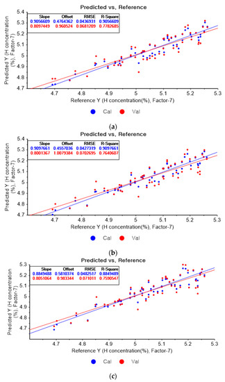
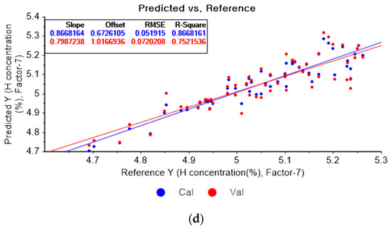
Figure 7.
PLSR model of hydrogen concentration with (a) original data and PLSR models pre-processed by SG smoothing using (b) first-order polynomial with one point, (c) first-order polynomial with three points, and (d) first-order polynomial with five points.
Figure 8a shows the PLSR model for hydrogen using the original data. Figure 8b–d present the pre-processed data by the SG second-order derivative using a second-order polynomial with one, three, and five smoothing points, respectively. In Figure 8a, the R2 of calibration, the R2 of cross-validation, the RMSEC, and the RMSECV are 0.90566, 0.77827, 0.04369, and 0.06812, respectively. As shown in Figure 8b, the R2 of calibration, the R2 of cross-validation, the RMSEC, and the RMSECV are 0.95064, 0.786515, 0.03160, and 0.05312, respectively. In Figure 8c, the R2 of calibration, the R2 of cross-validation, the RMSEC, and the RMSECV are 0.91928, 0.82983, 0.04042, and 0.05968, respectively. In Figure 8d, the R2 of calibration, the R2 of cross-validation, the RMSEC, and the RMSECV are 0.90873, 0.81504, 0.04298, and 0.06222, respectively. When the PLSR models are constructed with the original data, the data preprocessed by the SG-smoothing method, and the data pre-treated by the SG derivative pre-processing method, the R2 of calibration, the R2 of cross-validation, the RMSEC, and the RMSECV values are improved to a greater degree by applying the SG derivative pre-processing method.
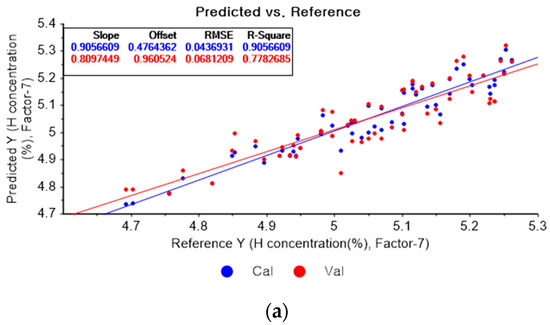
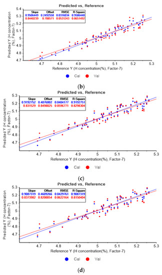
Figure 8.
PLSR model of hydrogen concentration with (a) original data and PLSR models pre-processed by SG derivative using (b) second-order derivative and second-order polynomial with one point, (c) second-order derivative and second-order polynomial with three points, and (d) second-order derivative and second-order polynomial with five points.
The measured and predicted hydrogen concentrations are presented in Figure 9. The maximum relative errors in the PLSR model were 1.74, 1.71, and 1.17% with the original data, those preprocessed by SG smoothing, and those preprocessed by the SG derivative method, respectively. The relative errors seemed quite low.
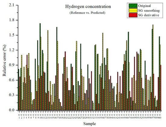
Figure 9.
Comparison of relative errors between measured and predicted hydrogen concentrations for the PLSR models with the original data and pre-processed data.
Figure 10a represents the results of the PLSR model for oxygen using the original data. Figure 10b–d represent the results of the PLSR models pre-processed by SG smoothing-based pre-processing using a fourth-order polynomial with one, three, and five smoothing points, respectively. In Figure 10a, the R2 of calibration, the R2 of cross-validation, the RMSEC, and the RMSECV are 0.84080, 0.72224, 1.00630, and 1.35176, respectively. As shown in Figure 10b, the R2 values of calibration and cross-validation, the RMSEC, and the RMSECV are 0.83960, 0.71873, 1.01011, and 1.36027, respectively. In Figure 10c, the R2 values of calibration and cross-validation, the RMSEC, and the RMSECV are 0.83424, 0.71612, 1.02684, and 1.36656, respectively. In Figure 10d, the R2 values of calibration and cross-validation, the RMSEC, and the RMSECV are 0.83010, 0.71803, 1.03959, and 1.36196, respectively. Regarding the oxygen concentration estimation pre-processed by the SG-smoothing method, the R2 values of calibration and cross-validation, the RMSEC, and the RMSECV values were decreased.
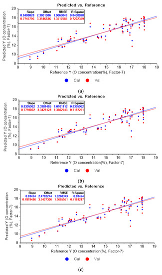
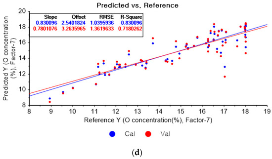
Figure 10.
PLSR model of oxygen concentration using the (a) original data and PLSR models pre-processed by SG smoothing using (b) fourth-order polynomial with three points, (c) fourth-order polynomial with five points, and (d) fourth-order polynomial with seven points.
Figure 11a shows the results of the PLSR model for oxygen constructed with the original data. Figure 11b–d represent the PLSR models pre-processed by the SG derivative using the third-order derivative and fifth-order polynomial with three, five, and seven smoothing points, respectively. In Figure 11a, the R2 values of calibration and cross-validation, the RMSEC, and the RMSECV are 0.84080, 0.72224, 1.00630, and 1.35176, respectively. As shown in Figure 11b, the R2 values of calibration and cross-validation, the RMSEC, and the RMSECV are 0.87822, 0.70052, 0.88015, and 1.40361, respectively. In Figure 11c, the R2 values of calibration and cross-validation, the RMSEC, and the RMSECV are 0.84977, 0.71277, 0.97757, and 1.37459, respectively. In Figure 11d, the R2 values of calibration, and cross-validation, the RMSEC, and the RMSECV are 0.81573, 0.66723, 1.08264, and 1.47957, respectively. The PLSR model pre-processed by the SG derivative method resulted in the most improved R2 of calibration and RMSEC values.
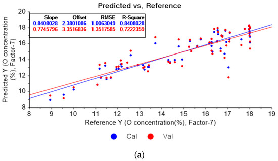
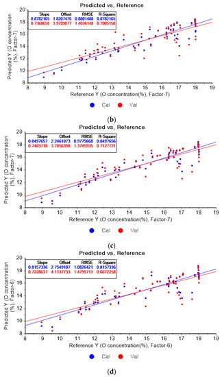
Figure 11.
PLSR model of oxygen concentration with the (a) original data and PLSR models pre-processed by SG derivative using (b) third-order derivative and fifth-order polynomial with three points, (c) third-order derivative and fifth-order polynomial with five points, and (d) third-order derivative and fifth-order polynomial with seven points.
The measured oxygen concentration and the predicted oxygen concentration are presented in Figure 12. The maximum relative errors were 23.52, 23.16, and 17.56% in the PLSR models using the original data and the PLSR models pre-processed by SG smoothing and the SG derivative, respectively. The PLSR model pre-processed by the SG derivative showed a low relative error.
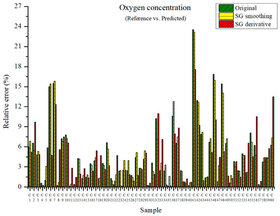
Figure 12.
Comparison of relative errors between measured and predicted oxygen concentrations for the PLSR models employing the original data and pre-processed data.
Figure 13a represents the PLSR model for sulfur using the original data. Figure 13b–d represent the PLSR models pre-processed by the SG-smoothing-based preprocessing method using third-order polynomials with three, five, and seven smoothing points, respectively. In Figure 13, the R2 values of calibration and cross-validation, the RMSEC, and the RMSECV are 0.92651, 0.89814, 0.07462, and 0.08934, respectively. As shown in Figure 13b, the R2 values of calibration and cross-validation, the RMSEC, and the RMSECV are 0.94079, 0.91460, 0.06699, and 0.08181, respectively. In Figure 13c, the R2 values of calibration and cross-validation, the RMSEC, and the RMSECV are 0.94820, 0.91692, 0.06265, and 0.08069, respectively. In Figure 13d, the R2 values of calibration and cross-validation, the RMSEC, and the RMSECV are 0.94472, 0.90623, 0.06472, and 0.08573, respectively. As shown in Figure 13b, the R2 of calibration and the RMSEC values are improved to a greater degree in the PLSR model. The RMSECV value of the R2 of cross-validation is slightly improved with the adoption of the PLSR model, as shown in Figure 13d.
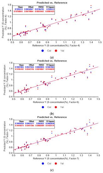
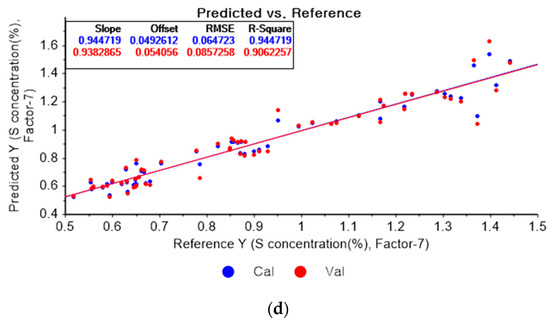
Figure 13.
PLSR model of sulfur concentration with (a) the original data and PLSR models pre-processed by SG smoothing using (b) third-order polynomial with three points, (c) third-order polynomial with five points, and (d) third-order polynomial with seven points.
Figure 14a depicts the PLSR model for sulfur using the original data. Figure 14b–d show the PLSR models pre-processed by the SG derivative using the second-order derivative and second-order polynomials with one, three, and five smoothing points, respectively. In Figure 14a, the R2 values of calibration and cross-validation, the RMSEC, and the RMSECV are 0.92651, 0.89814, 0.07462, and 0.08934, respectively. As shown in Figure 14b, the R2 values of calibration, and cross-validation, the RMSEC, and the RMSECV are 0.96412, 0.2382, 0.05214, and 0.07727, respectively. In Figure 14c, the R2 values of calibration and cross-validation, the RMSEC, and the RMSECV are 0.93791, 0.90530, 0.06893, and 0.08615, respectively. In Figure 14d, the R2 values of calibration and cross-validation, the RMSEC, and the RMSECV are 0.93119, 0.89697, 0.07221, and 0.08986, respectively. When the PLSR models pre-processed by SG smoothing and the SG derivative are compared with the PLSR model using the original data, the R2 values of calibration and cross-validation, the RMSEC, and the RMSECV in the PLSR models pre-processed by the SG derivative method are significantly improved.
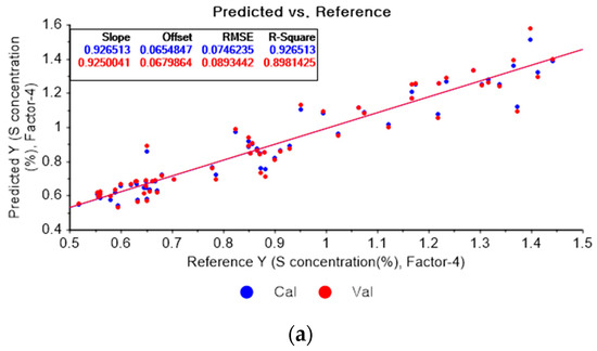
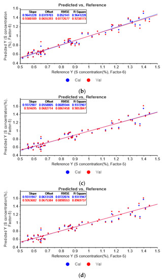
Figure 14.
PLSR model of sulfur concentration employing the (a) original data and PLSR models pre-processed by SG derivative using (b) second-order derivative and second-order polynomial with one point, (c) second-order derivative and second-order polynomial with three points, and (d) second-order derivative and second-order polynomial with five points.
The measured and predicted sulfur concentrations are presented in Figure 15. The maximum relative errors were 32.11, 20.13, and 18.84% for the PLSR model using the original data and the PLSR models pre-processed by the SG-smoothing and SG derivative methods, respectively. The relative error was the lowest in the PLSR model that adopted the SG derivative method.
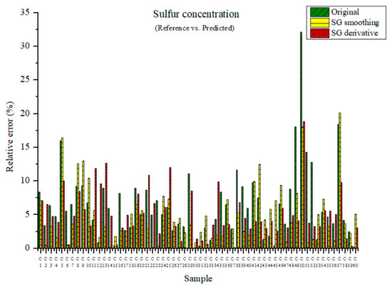
Figure 15.
Comparison of relative errors between measured and predicted sulfur concentrations for the PLSR models using the original data and pre-processed data.
3.1.2. Root Mean Square Error (RMSE) Average of Major Elements of Mixed Coals
The average RMSE (%) can be obtained from the RMSE values of the PLSR models for the major elements in mixed coal. The average RMSE (%) can be defined by the following equation:
where the average of property is the mean value of each elemental concentration used as the reference value. As shown in Table 1, the RMSEC (avg.) and RMSECV (avg.) were 0.7570 and 0.9538 in the original data for carbon. For the carbon data pre-processed by SG smoothing, the RMSEC (avg.) and RMSECV (avg.) were 0.7089 and 0.9080, respectively. The RMSEC (avg.) and RMSECV (avg.) (%) were 0.6229 and 1.0064 for the carbon data pre-processed by the SG derivative, respectively. The RMSECV (avg.) value was the lowest with SG smoothing. The RMSEC (avg.) and RMSECV (avg.) in the original data for hydrogen are 0.8652 and 1.3489, respectively. The RMSEC (avg.) and RMSECV (avg.) in the SG-smoothing data are 0.8461 and 1.3914, respectively. The values of the RMSEC (avg.) and RMSECV (avg.) were 0.6258 and 1.0519 with the SG derivative method, respectively. The RMSEC (avg.) and RMSECV (avg.) with SG derivate method could be improved. In the case of oxygen, the RMSEC (avg.) and RMSECV (avg.) are 6.7308 and 9.0414 in the original data, respectively. The RMSEC (avg.) and RMSECV (avg.) with the SG-smoothing method are 6.7563 and 9.0984, respectively. The RMSEC (avg.) (%) and RMSECV (avg.) were 5.8870 and 9.3883 with the SG derivative method, respectively. The RMSECV (avg.) was the lowest for the original data. In the case of sulfur, the RMSEC (avg.) and RMSECV (avg.) were 7.6019 and 9.1453, respectively. The RMSEC (avg.) and RMSECV (avg.) with the SG-smoothing method were 7.5097 and 9.0301, respectively. The RMSEC (avg.) and RMSECV (avg.) were 5.8513 and 8.6710 with the SG derivative method, respectively. The RMSEC (avg.) and RMSECV (avg.) with the SG derivate method were slightly improved.

Table 1.
Comparison of RMSE average (%) of mixed coal elements between original data and pre-processed data.
3.1.3. Residual Predictive Deviation (RPD) of Major Elements of Mixed Coals
The residual predictive deviation (RPD) parameter was introduced to examine the accuracy of the PLSR model and can be defined by the following equation:
where SD is the standard deviation of each element’s concentration obtained from conventional industrial analysis, and RMSECV is the RMSE of cross-validation for the PLSR. When the RPD is lower than 2.0, the model is considered as insufficient. When the RPD lie between 2.0 and 2.5, the model is approximately precise and is recommended for use in the estimation of composition. When the RPD is in the range from 2.5 to 3.0, the model is very precise. When the RPD is higher than 3.0, the model is considered as an excellent model [18,19,20].
In Table 2, the PLSR model of each element after the application of the SG derivative method shows that the RPD values of carbon and hydrogen are 3.10 and 2.63. Thus, both of the PLSR models are considered to be sufficiently precise. The RPD of oxygen is 1.70, which indicates that the PLSR model for oxygen is insufficient. However, the RPD of sulfur is 3.53, which proves that the PLSR model for sulfur is excellent, although the sulfur concentration is extremely low compared to the concentrations of other elements.
Table 2.
RPD of mixed coal.
3.2. Calorific Value Analysis
Since coal is used as the main fuel in coal-fired power generation, the calorific value of coal is a very important factor. Water vapor, which is a by-product of coal combustion, has latent heat. Therefore, a higher heating value (HHV) including the latent heat of steam is appropriate for the estimation of the calorific value of coal. The PLSR model was used to estimate the concentration of each element. The predicted calorific value can be obtained by substituting the predicted concentration of elements such as carbon, hydrogen, oxygen, and sulfur into Dulong’s equation, which is a higher heating value equation [21]:
where, C, H, O, and S are the concentrations (%) of carbon, hydrogen, oxygen, and sulfur, respectively. The calorific value obtained from the Daedeok Analytical Research Institute via industrial analysis was compared with the calorific value estimated from the PLSR models of each element shown above.
Figure 16 shows the relative errors between the measured and predicted values for the PLSR model using the original data and the PLSR model pre-processed by the SG derivative method [22]. The predicted calorific value was obtained by substituting the concentration of the elements from the PLSR model into Equation (5), i.e., the higher heating value equation. The relative error of the original data ranged from 0.09 to 6.45% and the average relative error was 2.22%. The relative errors of the PLSR model pre-processed by the SG derivative varied from 0.02 to 5.54% and the average relative error was 2.18%. They are slightly improved when they are compared with the relative errors of the original data in the range from 0.09 to 6.45%, as shown in Figure 16. The mean relative error of 2.18% was smaller than that of 2.22% obtained from the result of Figure 16. Therefore, the prediction of calorific value via the SG derivative method provides more reliable values.
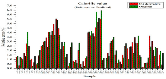
Figure 16.
Relative errors between measured and predicted values for the PLSR model of the original data and the PLSR model pre-processed by SG derivative.
4. Conclusions
Multivariate analyses for the carbon, hydrogen, oxygen, and sulfur components of mixed coals measured by LIBS were quantitatively analyzed. The data treated by SG smoothing and the SG derivative were adopted in the PLSR models. The coefficient of determination (R2), the root mean square error, the relative error, and the RMSE average were adopted as parameters. The most reliable PLSR model was selected by introducing the RPD parameter. The concentration of each element was predicted by the selected PLSR model, and the calorific value was obtained by using the estimated concentration of elements and substituting them into Dulong’s equation. The data pre-processed with the SG derivative showed better results regarding the calorific value of the mixed coals.
Author Contributions
Conceptualization, J.H.P. and S.J.M.; methodology, J.H.P.; software, K.H.P. and C.M.R.; validation, K.H.P.; formal analysis, J.H.P.; investigation, C.M.R. and K.H.P.; data curation, C.M.R.; resources, J.H.C.; funding—acquisition, S.J.M. and J.H.C.; writing—original draft preparation, J.H.P.; writing—review and editing, J.H.C., S.J.M. and K.H.P.; visualization, C.M.R.; supervision, S.J.M.; All authors have read and agreed to the published version of the manuscript.
Funding
This work was partially supported by the Technology Innovation Program (or Industrial Strategic Technology Development Program—Development of technical support platform for welding material and process) (20017251, Development of laser-welding automation systems for electric coil-joining system to manufacture electrical vehicle motors) funded By the Ministry of Trade, Industry, and Energy (MOTIE, Republic of Korea). This work was partially supported by the National Research Foundation of Korea (NRF) entitled “Development of Coal Analyzing System Using Laser-induced Breakdown Spectroscopy for Clean Coal Power Plant“ (No. NRF-2016R1D1A1B03935556). This work was partially supported by the Basic Science Research Program through the National Research Foundation (NRF) of Korea entitled “NRF-2016R1D1A1B04934910”.
Conflicts of Interest
The authors declare no conflict of interest. The funders had no role in the design of the study; in the collection, analyses, or interpretation of data; in the writing of the manuscript, or in the decision to publish the results.
References
- Korea Energy Economics Institute. Yearbook of Energy Statics; Korea Energy Economics Institute: Ulsan, Republic of Korea, 2017; pp. 180–181. [Google Scholar]
- Wang, Z.; Dong, F.; Zhou, W. A rising force for the world-wide development of laser-induced breakdown spectroscopy. Plasma Sci. Technol. 2015, 8, 617–620. [Google Scholar] [CrossRef]
- Wilde, H.R.; Herzog, W. On-line analysis of coal by neutron induced gamma spectrometry. J. Radioanal. Chem. 1982, 71, 253–264. [Google Scholar] [CrossRef]
- Zhang, Y.S.; Lee, J.T.; Hwang, S.W.; Jin, Y.I.; Park, C.W.; Moon, Y.H. Quantitative Elemental Analysis in Soils by using Laser Induced Breakdown Spectroscopy(LIBS). Korean J. Soil Sci. Fertil. 2009, 42, 399–407. [Google Scholar]
- Fichet, P.; Mauchien, P.; Wagner, J.F.; Moulin, C. Quantitative elemental determination in water and oil by laser induced breakdown spectroscopy. Anal. Chim. Acta 2001, 429, 269–278. [Google Scholar] [CrossRef]
- Davari, S.A.; Hu, S.; Pamu, R.; Mukherjee, D. Calibration-free quantitative analysis of thin-film oxide layers in semiconductors using laser induced breakdown spectroscopy (LIBS). J. Anal. At. Spectrom. 2017, 32, 1378–1387. [Google Scholar] [CrossRef]
- Yao, S.; Lu, J.; Dong, M.; Chen, K.; Li, J.; Li, J. Extracting coal ash content from laser-induced breakdown spectroscopy (LIBS) spectra by multivariate analysis. Appl. Spectrosc. 2011, 65, 1197–1201. [Google Scholar] [CrossRef] [PubMed]
- Yuan, T.; Wang, Z.; Lui, S.L.; Fu, Y.; Li, Z.; Liu, J.; Ni, W. Coal property analysis using laser-induced breakdown spectroscopy. J. Anal. At. Spectrom. 2013, 28, 1045–1053. [Google Scholar] [CrossRef]
- Dong, M.; Lu, J.; Yao, S.; Li, J.; Li, J.; Zhong, Z.; Lu, W. Application of LIBS for direct determination of volatile matter content in coal. J. Anal. At. Spectrom. 2011, 26, 2183–2188. [Google Scholar] [CrossRef]
- Liangying, Y.; Jidong, L.; Wen, C.; Ge, W.; Kai, S.; Wei, F. Analysis of Pulverized Coal by Laser-Induced Breakdown Spectroscopy. Plasma Sci. Technol. 2005, 7, 3041–3044. [Google Scholar] [CrossRef]
- Wang, Z.; Yuan, T.B.; Lui, S.L.; Hou, Z.Y.; Li, X.W.; Li, Z.; Ni, W.D. Major elements analysis in bituminous coals under different ambient gases by laser-induced breakdown spectroscopy with PLS modeling. Front. Phys. 2012, 7, 708–713. [Google Scholar] [CrossRef]
- Pei, L.; Jiang, G.; Tyler, B.J.; Baxter, L.L.; Linford, M.R. Time-of-flight secondary ion mass spectrometry of a range of coal samples: A chemometrics (PCA, cluster, and PLS) analysis. Energy Fuels 2008, 22, 1059–1072. [Google Scholar] [CrossRef]
- Bona, M.T.; Andrés, J.M. Reflection and transmission mid-infrared spectroscopy for rapid determination of coal properties by multivariate analysis. Talanta 2008, 74, 998–1007. [Google Scholar] [CrossRef] [PubMed]
- Wang, Y.; Yang, M.; Wei, G.; Hu, R.; Luo, Z.; Li, G. Improved PLS regression based on SVM classification for rapid analysis of coal properties by near-infrared reflectance spectroscopy. Sens. Actuators B Chem. 2014, 193, 723–729. [Google Scholar] [CrossRef]
- Li, W.; Lu, J.; Dong, M.; Lu, S.; Yu, J.; Li, S.; Huang, J.; Liu, J. Quantitative Analysis of Calorific Value of Coal Based on Spectral Preprocessing by Laser-Induced Breakdown Spectroscopy (LIBS). Energy Fuels 2018, 32, 24–32. [Google Scholar] [CrossRef]
- Lee, Y.; Choi, D.; Gong, Y.; Nam, S.-H.; Nah, C. Laser-induced plasma emission spectra of halogens in the helium gas flow and pulsed jet. Anal. Sci. Technol. 2013, 26, 235–244. [Google Scholar] [CrossRef]
- Galtier, O.; Abbas, O.; Le Dréau, Y.; Rebufa, C.; Kister, J.; Artaud, J.; Dupuy, N. Comparison of PLS1-DA, PLS2-DA and SIMCA for classification by origin of crude petroleum oils by MIR and virgin olive oils by NIR for different spectral regions. Vib. Spectrosc. 2011, 55, 132–140. [Google Scholar] [CrossRef]
- Martelo-Vidal, M.J.; Vázquez, M. Determination of polyphenolic compounds of red wines by UV–VIS–NIR spectroscopy and chemometrics tools. Food Chem. 2014, 158, 28–34. [Google Scholar] [CrossRef]
- Aleixandre-Tudó, J.L.; Alvarez, I.; García, M.J.; Lizama, V.; Aleixandre, J.L. Application of multivariate regression methods to predict sensory quality of red wines. Food Sci. 2015, 33, 217–227. [Google Scholar] [CrossRef]
- Wu, Z.; Xu, E.; Long, J.; Zhang, Y.; Wang, F.; Xu, X.; Jin, Z.; Jiao, A. Monitoring of fermentation process parameters of Chinese rice wine using attenuated total reflectance mid-infrared spectroscopy. Food Control 2015, 50, 405–412. [Google Scholar] [CrossRef]
- Kathiravale, S.; Yunus, M.N.M.; Sopian, K.; Samsuddin, A.H.; Rahman, R.A. Modeling the heating value of Municipal Solid Waste. Fuel 2003, 82, 1119–1125. [Google Scholar] [CrossRef]
- Sanghapi, H.K.; Jain, J.; Bol’Shakov, A.; Lopano, C.; McIntyre, D.; Russo, R. Determination of elemental composition of shale rocks by laser induced breakdown spectroscopy. Spectrochim. Acta-Part B At. Spectrosc. 2016, 122, 9–14. [Google Scholar] [CrossRef]


Disclaimer/Publisher’s Note: The statements, opinions and data contained in all publications are solely those of the individual author(s) and contributor(s) and not of MDPI and/or the editor(s). MDPI and/or the editor(s) disclaim responsibility for any injury to people or property resulting from any ideas, methods, instructions or products referred to in the content. |
© 2022 by the authors. Licensee MDPI, Basel, Switzerland. This article is an open access article distributed under the terms and conditions of the Creative Commons Attribution (CC BY) license (https://creativecommons.org/licenses/by/4.0/).