Abstract
Unsupervised domain adaptation involves knowledge transfer from a labeled source to unlabeled target domains to assist target learning tasks. A critical aspect of unsupervised domain adaptation is the learning of more transferable and distinct feature representations from different domains. Although previous investigations, using, for example, CNN-based and auto-encoder-based methods, have produced remarkable results in domain adaptation, there are still two main problems that occur with these methods. The first is a training problem for deep neural networks; some optimization methods are ineffective when applied to unsupervised deep networks for domain adaptation tasks. The second problem that arises is that redundancy of image data results in performance degradation in feature learning for domain adaptation. To address these problems, in this paper, we propose an unsupervised domain adaptation method with a stacked convolutional sparse autoencoder, which is based on performing layer projection from the original data to obtain higher-level representations for unsupervised domain adaptation. More specifically, in a convolutional neural network, lower layers generate more discriminative features whose kernels are learned via a sparse autoencoder. A reconstruction independent component analysis optimization algorithm was introduced to perform individual component analysis on the input data. Experiments undertaken demonstrated superior classification performance of up to 89.3% in terms of accuracy compared to several state-of-the-art domain adaptation methods, such as SSRLDA and TLMRA.
1. Introduction
An assumption of traditional machine learning classification methods is that training and test data have independent and identical distributions [1]. Because different domains are usually different but related in real-world scenarios, most existing traditional machine learning methods are not guaranteed to be effective due to the ubiquitous large discrepancy between different domains [2,3]. To address this problem, in recent decades, domain adaptation methods have attracted a great deal of attention and stimulated research studies [4,5,6,7], which have primarily focused on the transfer of knowledge between different domains. Because the target domain is usually unknown, unsupervised domain adaptation aims to promote learning tasks in target domains based on knowledge in source domains, which has far-ranging consequences for practical applications, such as speech emotion recognition [8], medical image classification [9], and semantic image segmentation [9].
Among domain adaptation methods, including instance-transfer, parameter-transfer, feature-representation-transfer and relational-knowledge-transfer methods [10], methods based on feature representation learning can be applied to a broader set of scenarios due to loose restrictions on source data [11]. The key issue for feature-representation-transfer methods is how to learn more discriminative and transferable feature representations to minimize deviations between different domains [12].
In recent decades, remarkable progress has been made in the use of feature learning methods based on shallow structure and deep neural networks which have learned how to transfer representations across domains and have performed well in unsupervised domain adaptation. Typical shallow learning methods, such as transfer component analysis [13], aim to reduce domain divergence in new feature space using a kernel function. In comparison to shallow structure methods, deep neural networks have been shown to be more effective by separating the explanatory factors behind different domains [14,15]. Recently, mainstream deep neural networks, such as the convolutional neural network (CNN) [16], the recurrent neural network (RNN) [17], the generative adversarial network (GAN) [18], and Autoencoder [19], have been used to learn more discriminative representations for unsupervised domain adaptation and have performed well in reducing domain divergence.
Among unsupervised domain adaptation methods that are based on deep neural networks, the autoencoder-based method has achieved superior performance with respect to the no label requirement and fast convergence speed. For example, the stacked denoising autoencoder (SDA) method [20] aims to learn higher-level representations from all available domains to train a classifier that performs classification on new-featured spaces. Similarly, to address the issue of high computational cost in SDA, a marginalized stacked denoising autoencoder method [19] has been proposed based on matrix computation, which is as effective as SDA in representation learning for domain adaptation and has been shown to be more efficient. In light of the development of these methods, Wei et al. proposed an unsupervised domain adaptation method based on non-linear representation learning [21], which introduced non-linear coding by kernelization into SDA to enable the extraction of deep features.
While it is possible to explore different domains and learn transferable and discriminative representations using unsupervised domain adaptation methods based on autoencoders, most current approaches depend on use of the classical structure of autoencoders or integration of regularization terms into the objective function [22,23,24]. For improved understanding of feature representation learning, here, a method is proposed to achieve representation learning based on a stacked convolutional sparse autoencoder for unsupervised domain adaptation, which can capture more transferable and distinguishable features by layer mapping of the raw data and unsupervised domain adaptation. Firstly, we utilize the reconstruction independent component analysis (RICA) algorithm [4] with whitening to pre-process the original data in both source and target domains, where “whitening” refers to a transformation of the original data x to , and the covariance matrix of is the identity matrix. A stacked sparse autoencoder is then introduced to extract features to alleviate domain discrepancy. Secondly, based on the new feature space learned by the first component, convolution and pooling are applied to maintain local relevance. Finally, we stack two convolutional sparse autoencoders to achieve more abstract and transferable representation learning. Compared to other state-of-the-art methods, experimental results obtained confirm the effectiveness of our proposed framework for unsupervised domain adaptation.
In summary, this paper makes the following main contributions:
- We explicitly propose a new framework of unsupervised domain adaptation based on a stacked convolutional sparse autoencoder (short for SCSA). There is an obvious distinction between this method and the original method [2,14], which relies on applying the classical structure of the autoencoder to learn representations or integratation of the regularization term into the objective function.
- Our proposed SCSA has two main components in each layer. In the first component, a stacked sparse autoencoder with RICA is introduced for recognition feature learning to reduce the divergence between the source and target domains. In the second component, the convolution and pool layer is utilized to preserve the local relevance of features to achieve enhanced performance.
The remainder of the paper is organized as follows: In Section 2, related work is described. In Section 3, the SCSA proposal is described in detail. Several real-world datasets are presented and the experimental results are analyzed in Section 4. The conclusions are presented in Section 5.
It is worth explaining that we first introduced the unsupervised domain adaptation method in our conference paper [25], titled “Domain Adaptation with Stacked Convolutional Sparse Autoencoder”, published in the proceedings of the Twenty-Eighth International Conference on Neural Information Processing (ICONIP), Indonesia, 8–12 December 2021. In our conference paper, we focus on a domain adaptation method with an autoencoder (SCSA). Here, we propose an unsupervised domain adaptation framework. Compared with our previous version, we add the following: (1) further discussion and analysis regarding validation of the proposed method; (2) more detailed description of the proposed method; (3) a more comprehensive survey of related studies; and (4) further experimental analysis of the SCSA and the baselines.
2. Background Studies
Due to strong feature representation learning ability, deep neural networks have attracted considerable attention regarding domain adaptation. For example, Ganin et al. proposed an unsupervised domain adaptation method with deep architectures [26], which trained a model with standard back-propagation on large-scale labeled source data and unlabeled target data. Similarly, Sener et al. proposed a fine-tuned deep neural network to minimize the discrepancy between different domains [27]. An end-to-end model was designed to jointly optimize learned features, to cross-domain transform, and target label prediction. Existing deep domain adaptation methods can be broadly categorized into three classes: discrepancy-based, adversarial-based and PLM-based methods [28].
Discrepancy-based methods aim to embed data from source and target domains into a kernel space to alleviate domain discrepancy. For example, Zhang et al. proposed a deep neural network based on the maximum mean discrepancy (MMD) [29], which was able to learn a common subspace to simultaneously align both marginal and conditional distributions. Long et al. proposed a residual transfer network [30], which not only aligned the feature distributions between different domains, but also transferred the classifier with a residual function. As well as these deep methods, which mainly focus on cross-feature learning, many methods have been proposed to transfer the classifier across different domains. For example, Pinheiro proposed training the classifier with similarity learning [31]; application of this method demonstrated that feature representation learning together with similarity learning can improve domain adaptation.
Inspired by the generative adversarial net (GAN) approach, adversarial-based domain adaptation methods aim to minimize deviations across domains using an adversarial objective. For example, Long et al. designed a conditional domain adversarial network [32], which conditions adversarial adaptation models based on the discriminative information conveyed in the classifier predictions. Kang et al. proposed a contrastive adaptation network for minimizing intra- and inter-class deviations [7], which included an end-to-end update strategy for model optimization. Pei et al. proposed a multi-adversarial domain adaptation method [33]. In this method, multiple class-wise domain discriminators are constructed to reduce the shift of joint distributions between different domains and to achieve fine-grained alignment of different class distributions. In this way, each discriminator only matches samples of source and target data belonging to the same class.
Recently, pre-trained language models (PLMs) have received much attention and achieved remarkable improvements in a series of tasks. As PLMs can learn syntactic, semantic and structural information, there has been some effort to apply PLMs to domain adaptation. For example, Zhang et al. proposed a domain adaptation neural network based on BERT for multi-modal fake-news detection [34]. The pre-trained BERT and VGG-19 model were first introduced to learn text and image features, respectively. Then the multi-modal features were mapped onto the same space by domain adaptation. Finally, a detector was used to distinguish fake news. Guo et al. proposed the creation of input disturbance vectors using soft prompt tuning to optimize domain similarity [35], introducing targeted regularization to minimize domain discrepancy.
Although the deep learning methods described have achieved fairly good results in domain adaptation, the deep neural network training problem remains. Some efficient models, such as graph regularization and sparse constraint, cannot be applied directly in supervised convolutional networks. Moreover, although some optimization methods have been proposed, they have not been shown to be effective in unsupervised deep networks for domain adaptation tasks.
3. Related Work
The goal of domain adaptation is to reduce the discrepancy between different domains and to bridge the chasm among them. Amongst unsupervised domain adaptation methods, methods based on feature learning have been widely applied in multiple disciplines a a result of looser limitations on the data in the source domain. According to the technology used, existing feature-learning-based methods for domain adaptation can be broadly divided into two categories: shallow-learning and deep-learning methods.
3.1. Shallow Learning Methods
Among unsupervised domain adaptation methods based on shallow structure, the transfer component analysis (TCA) model [13] is a typical model that attempts to minimize the distance between source and target domains in a new feature space using the maximum mean discrepancy (MMD). Chen et al. proposed an unsupervised domain adaptation method based on an extreme learning machine network to retain the space information of the target domain [36], which seeks to transfer the source domain for better matching of the data distribution in the target domain by reducing the MMD distance. He et al. proposed an unsupervised domain adaptation model for multi-view data [37]; the features extracted from one view of the data are considered privileged information from another view. Chen et al. proposed combination of domain-adversarial learning and self-training with the intention of combining the strengths of both methods [38]. The pseudo-label prediction and the confusion matrix were learned using self-training and using an adversarial approach, respectively. Wang et al. proposed a symmetric and positive-definite matrix network for domain adaptation (daSPDnet) [39]. Inspired by Riemannian manifold methods, daSPDnet aims to enable EEG emotion recognition by overcoming the variability in the physiological responses of subjects.
Some effort has already been invested in applying unsupervised transfer methods to heterogeneous domains. For example, Liu et al. proposed a heterogeneous unsupervised domain adaptation model [40], which introduced an n-dimensional metric of fuzzy geometry to compute the similarity between different vectors. Based on the results, the fuzzy equivalence relations were explored and the cross-domain clustering categories were captured. Yan et al. proposed an optimal matrix transport method for heterogeneous domain adaptation [41], which introduced the entropic Gromov–Wasserstein discrepancy for learning an optimal transport matrix. Luo et al. proposed a distance metric learning method for heterogeneous domain adaptation [42]. This method used existing models to learn the knowledge fragments in the source domain, which can reduce domain divergence.
However, unsupervised domain adaptation methods based on shallow structure have two main drawbacks. The first is utilization of labeled data information, since a small amount of labeled data can significantly improve domain adaptation performance. The second drawback is the capacity for feature learning. How to learn more transferable representations to alleviate domain discrepancy represents a major challenge.
3.2. Autoencoder-Based Methods
Among deep neural networks, autoencoder-based unsupervised domain adaptation methods have performed well with respect to the no label requirement and fast convergence speed. For example, Glorot et al. proposed a stacked denoising autoencoder (SDA) for domain adaptation [43]. A marginalized denoising autoencoder (mSDA) method was proposed for speeding up SDA by two orders of magnitude [19]. Wei et al. introduced non-linear coding by kernelization into the mSDA for domain adaptation [21]. Zhuang et al. proposed an unsupervised domain adaptation framework with deep autoencoders [22]. In this method, the mSDA is utilized to pre-train the whole framework and two encoding and decoding layers are incorporated to learn more transferable representations between the source and target domains. Zhu et al. proposed integration of the manifold regularization term in the objective function [2], involving stacking of two layers of autoencoders to learn more abstract representations for unsupervised domain adaptation. Yang et al. proposed a semi-supervised method using dual autoencoders [1], which extracted more powerful features using two different autoencoders based on mSDA for unsupervised domain adaptation. Nikisins et al. proposed a face presentation attack detection model using an autoencoder and a multi-layer perceptron [44], which transferred the knowledge of facial appearance between different domains. This domain adaptation method reduced the requirements for large-scale labeled data, which avoided labor-intensive work and reduced costs when training face recognition systems. Zhu et al. proposed a deep sparse autoencoder for an imbalanced domain adaptation problem [45], which could adjust the model automatically according to the degree of imbalance to bridge the gap between domains. In this method, a self-adaptive imbalanced cross-entropy loss function is used to highlight minority categories and automatically compensate for training loss bias. In contrast to autoencoder-based methods that rely on application of the classical structure of an autoencoder to learn representations or integrate the regularization term into the objective function, our method introduces convolution and pooling kernels to use local relevance to learn abstract representations for domain adaptation.
4. Our Proposed Method
4.1. Motivation
For domain adaptation, methods based on feature representation learning can be applied to a broader set of scenarios because of the loose restrictions on the source data. Furthermore, among representation-learning-based domain adaptation methods, some typical supervised and unsupervised deep learning models, such as convolutional neural networks and the autoencoder, have achieved fairly good performance. However, there are two main problems that have prevented the further development of these methods. The first is the training problem associated with deep neural networks. Some efficient models, such as graph regularization and sparse constraint, cannot be applied directly in supervised convolutional networks. In addition, although some optimization methods have been proposed [46,47,48], they have not been demonstrated to be effective in unsupervised deep networks for domain adaptation tasks. The second problem is data redundancy of image data. As the adjacent pixels of an image inside a local area are highly correlated, high-dimensional features of image data are inevitably affected by performance degradation in representation learning. For example, in a local receptive field neural network, the local relationship of replication features leads to a non-uniform distribution of edge detectors. To address these two problems, we propose a stacked convolutional sparse autoencoder method for unsupervised domain adaptation. In contrast to previous autoencoder-based methods that rely on the classical structure or the integration of regularization terms into the objective function, path-wise training is used to optimize the model of the sparse autoencoder and then the convolutional kernels are used to reserve the local relevance for learning abstract representations. Furthermore, the reconstruction independent component analysis (RICA) algorithm with whitening is introduced to pre-process the original data in both the source and target domains to remove correlations inside the local area for representation learning.
In Figure 1, a stacked convolutional sparse autoencoder is illustrated as the proposed unsupervised domain adaptation method. The SCSA consists of several levels: for example, there are two layers in Figure 1; layer 2 is a repeat of layer 1 for more abstract feature learning; each layer is composed of two components. Firstly, the input data information is sphered according to the RICA with whitening. The overall goal of this part is to perform a separate part analysis of the imported data. Then, the transferable features are learned by training on patches with a sparse autoencoder. Secondly, the CNN feature maps are generated with the help of practical convolution operations and pooling in different domains. According to the projection layer, a classifier is built from the final features by transforming and reshaping them in the overall target domain.
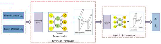
Figure 1.
Illustration of our proposed SCSA. Each layer is composed of two main components: a stacked sparse autoencoder and the convolution and pooling kernels. The whitening layer is first introduced for recognition feature learning.
4.2. Stacked Sparse Autoencoder
The first component is composed of a sparse autoencoder with a whitening layer that learns the latent feature representations from the data in the source domain. As the target domain is unlabeled in unsupervised domain adaptation, the source domain with labeled data and target domain with unlabeled data is with and , where and denote the instances in the source and target domain and and denote the number of instances in the source and target domain, respectively; denotes the label information in the source domain, m denotes the feature dimension of the input data and c denotes the number of labels. In a sparse autoencoder, at the encoder stage, the data from both the source and the overall target domains are projected onto vectors in the hidden layer, respectively, expressed as and . Then, in the decoder stage, the and are mapped to the output layer as and . To obtain more powerful feature representations for knowledge transfer, we introduce a softmax encoder weight regularization to apply the labeled information in the source domain to train the whole model.
First, we introduce the RICA algorithm to perform the independent component analysis from the original data in both source and target domains. We utilize the whitening layer before the RICA to make the input less redundant. The objective function can be shown as (1):
X denotes the original data in both source and target domains, denotes the weight matrix, and are the tuning parameters. To scale the reconstruction item, i.e., the second item in (1), the regularization expressed as is introduced to (1). In our method, we select as a small constant to prevent the regularization item from being numerically close to zero. Thus, (1) can be expressed as (2):
The partial derivatives of can be formalized as (3):
According to the partial derivatives of (3), the output of the RICA is fed into the next autoencoder as the input.
After the RICA, we introduce the stacked sparse autoencoder with softmax weight regression to learn more abstract features across the source and target domains. In the stacked sparse autoencoder, the desired partial derivatives regrading W and b can be shown as (4) and (5):
, and are the weight matrix, bias vector and output of the hidden level in the autoencoder, respectively. Taking the added sparsity penalty term in the sparse autoencoder into consideration, can be calculated in (6):
where . The output of the sparse autoencoder is represented as . Due to space limitation, more details for (4)–(6) are provided in Appendix A.
To utilize the labeled information in the source domain to alleviate domain discrepancy, we follow the approach used in [2]; the softmax encoder weight regularization is introduced into the stacked sparse autoencoder. The objective function is described in (7):
where and are the trade-off parameters, which aim to balance the effectiveness of each item in (7).
The second term in (7) is the cost function of the softmax encoder weight regularization, which can be formalized as (9):
where denotes the j-th row of , and denotes the label in the source domain.
As the objective function is an unconstrained optimization problem, the minimization of J with respect to , , , and is adopted using the l-bfgs method, which has been demonstrated to be a more efficient backtracking method [22]. The partial derivatives of can be formalized as (11):
The alternate optimization method is adopted to derive the solutions as follows:
, , where is the step length, which determines the speed of convergence.
4.3. Convolution and Pool Layer
After feature learning via the stacked sparse autoencoder, the convolution and pool kernel is utilized to preserve the local relevance of features. Given are the whole sample representation of both source and target domain maps of layer l, where and represent the height and width of each input map, respectively, and d represents the number of channels. The patches are extracted from to compose the training set for learning latent features, where K denotes the number of patches, and are the size of patches, respectively, and denotes the convolution kernel size. Each input is reshaped to the vector of for the convenience of training the autoencoder. The number of neurons in hidden layer l can be manually designed.
After the convolved features are extracted, we divide the input features into disjoint regions, and the mean (or maximum) activation function is utilized to obtain the pooled convolution feature representations, where and denote the size of patches. Different pooling methods are selected for different distributed datasets. For example, the mean pool objective function is (12):
In the experiments performed, the parameter in the objective function is updated as (13):
where is derived from the projection and is the learning rate, which is usually much lower than the corresponding learning rate in batch gradient descent due to larger variance in the update. In the experiments undertaken, the momentum method is introduced to rapidly facilitate the objective along the shallow ravine.
where v is the current velocity vector with the same dimension as the parameter vector . determines how many iterations from the previous gradients are incorporated into the current update.
It is of note that the pooling operation can both reduce the representation dimensions and select more significant features. For example, the pervasive pooling tools, such as max-pooling [49], mean-pooling [50] and stochastic pooling [51] have achieved promising performance in feature representation learning. Therefore, in the experiments, two different pooling tools, max and mean pooling, were used according to the distribution of the datasets.
5. Experiments
5.1. Datasets
Corel Data Sethttp://archive.ics.uci.edu/ml/datasets/Corel+Image+Features, accessed on 1 June 2022. In the experiments, two different top categories in the dataset, such as flower and traffic, were selected as positive and negative [4]. The source domain was built by randomly choosing a subcategory from flower and traffic and the target domain was built by choosing another subcategory from flower and traffic. In this way, 144 domain adaptation classification tasks were constructed.
ImageNet Data Sethttp://www.image-net.org/, accessed on 1 February 2021. In the experiments, five domains where the ImageNet data information was centralized were selected [52], including ambulance, taxi, jeep, minivan and scooter. The scooter is considered as a set of negative cases, randomly divided into four other datasets. To better build the classification, we randomly selected two domains from the four domains as the source domain and target domain, respectively. Therefore, 12 domain adaptation classification tasks were constructed in this way. The number of positive and negative instances in four domains was 1000, and the number of features was 900. Details of the ImageNet datasets used in the experiments are listed in Table 1.

Table 1.
Details of the ImageNet dataset used in our experiment.
Leaves Data Sethttp://www.cse.wustl.edu/mchen/, accessed on 1 January 2021. In this dataset, there are 100 plant species in total, divided into 32 genera, with 16 species for each genus [53]. In the experiments, we selected four different genera from this dataset and four class classification problems were constructed with 64-margin descriptors. Therefore, 12 domain adaptation classification tasks were constructed.
5.2. Compared Methods
The following baseline methods were compared with our proposed SCSA:
- The standard classifier without unsupervised domain adaptation technique; we introduced support vector machine (SVM) in the experiments.
- Transfer component analysis (TCA) [13], which aims to project the original data into the common latent feature space via dimension reduction for unsupervised domain adaptation.
- Marginalized stacked denoising autoencoders (mSDA) [19], which are elaborated to learn more abstract and invasive feature representations so that domain integration can be carried out.
- Transfer learning with deep autoencoders (TLDA) [14]. The dual-level autoencoder is designed to learn more transferable features for domain adaptation.
- Transfer learning with manifold regularized autoencoders (TLMRA) [2]. To obtain more abstract representations, the method combines manifold regularization and softmax weight regression.
- Semi-supervised representation learning framework via dual autoencoders (SSRLDA) [1]. The mSDA with adaptation distributions and multi-class marginalized denoising autoencoder are applied to obtain global and local features for unsupervised domain adaptation.
5.3. Experiment Settings
For the trade-off parameters, , and were set for the Corel and ImageNet datasets, while , and were set for the Leaves dataset in our experiments. The hyper-parameters in the convolutional layers, such as the total number of maps, the kernel size, and the pooling type and size, are shown in Table 2. Among the methods compared, the best parameters were measured in the experiments using the mSDA method http://multitask.cs.berkeley.edu, accessed on 1 February 2021. For TCA, the total number of latent subspace dimensions was intentionally fixed and the best results were reported. For TLDA, the main parameters of the default settings were reported in [14]. We implemented the source code of TLMRA and SSRLDA under optimal parameter settings.
Table 2.
Main configurations of SCSA on Datasets.
5.4. Experimental Results
All the experimental results for the three datasets are listed in Table 3. Our experiments were conducted five times and the results presented are the average performances of all domain adaptation tasks. Figure 2 and Figure 3 show the results for the ImageNet and Leaves datasets, respectively. The following conclusions are drawn from the experimental results:
Table 3.
Average accuracy on all three datasets (%).
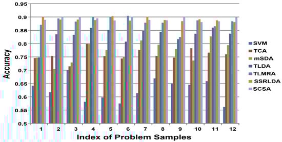
Figure 2.
Performances on ImageNet dataset. The y-axis represents the classification accuracy of the target domain; the x-axis represents the index of the problem sample.
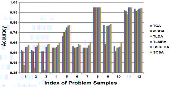
Figure 3.
Performances on Leaves dataset. The y-axis represents the classification accuracy of target domain; the x-axis represents the index of the problem sample.
- All the domain adaptation methods significantly and consistently outperformed the standard SVM classifier, demonstrating the advantages of the feature-representation method in a broader set of scenarios.
- Compared to shallow learning methods, such as TCA, autoencoder-based methods, such as TLDA, TLMRA, and SSRLDA, all achieved superior results in unsupervised domain adaptation, indicating the superiority of deep-learning-based methods in learning transferable and discriminative features across domains. Notably, mSDA achieved comparable performance to TCA, demonstrating that the traditional structure of the autoencoder cannot learn sufficient features. This is why other autoencoder-based methods require improvements in architecture.
- In comparison with mSDA, our SCSA achieved better performance in all tasks for three different datasets, demonstrating the superiority of our framework for exploring different domains compared to autoencoder-based domain adaptation methods.
- By comparison to other autoencoder-based deep methods, such as TLDA and TLMRA, our proposed SCSA achieved better performance for overall tasks in the same target domains and for the same problems. These methods rely on the classical structure of autoencoders (i.e., TLMRA) or the integration of regularization terms into the objective function (i.e., TLDA). The results confirm that our SCSA can explore abstract and distinctive features for domain adaptation.
- For all three experimental datasets, our method was better than SSRLDA. From Figure 2 and Figure 3, it can be seen that our method achieved better results for most tasks in the same target domains and for the same problems. Our SCSA also achieved comparable performance to SSRLDA in other tasks. As a semi-supervised method, our method achieved superior performance for all three image datasets, indicating that the convolution and pooling layer can maintain the local relevance and learn features better for domain adaptation in image datasets.
- Generally, compared with alternative methods, our SCSA achieved the best results in all groups for three different datasets, confirming the effectiveness of our proposed method.
5.5. Analysis of Properties in SCSA
SCSA with and without RICA: In our SCSA, the RICA with whitening played a foundation and optimization role in the experiments. Therefore, we conducted additional experiments to evaluate its optimizing ability. Table 4 shows the results for the SCSA with and without RICA for all three datasets. From the results, it can be observed that the proposed SCSA with RICA outperformed SCSA without RICA for all three datasets, indicating that the RICA can pre-process all the image datasets and make the input less redundant, which is obviously helpful for more transferable and discriminative feature learning. With less redundant input data, the cross-domain and invariant feature representations can improve performance in domain adaptation.
Table 4.
Average accuracy of SCSA without or with RICA for three datasets (%).
Computational Cost: The time complexity of a stacked sparse auto-encoder is , where and are the hidden unit numbers of two layers, respectively. For our method, we took the labeled information into consideration, given c as the number of classes; the time complexity is . For the convolution and pooling kernels, the time complexity is , where and represent the size of the input and the patches, respectively. The time complexity of our SCSA is .
5.6. Transfer Distance
The transfer distance that can be defined as the -distance is widely used as a similarity measure between the source and target domains [2,15,54]. The -distance can be defined as , where is the generalization error of classifiers, such as the linear SVM trained on the binary classification problem, which is used to distinguish the source domain from the target domain. If the new features are more suitable for domain adaptation tasks, the -distance increases in the new representation space. The results on the Corel and ImageNet datasets with and without our proposed SCSA are shown in Figure 4. It can be observed that the distance increases with the new features after the proposed method is applied. It appears that the representations obtained by SCSA are more appropriate for transfer learning applications.
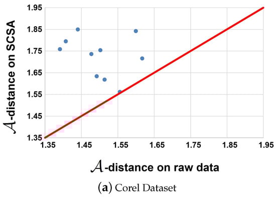
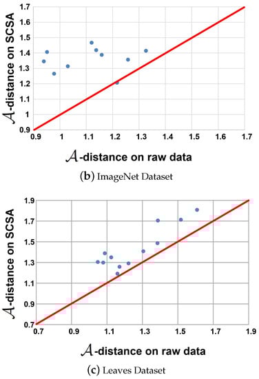
Figure 4.
-distance on Corel, ImageNet and Corel datasets. The x-axis and y-axis represent the -distance on the raw data and learned features space.
5.7. Parameter Sensitivity
The influence of hyper-parameters is investigated in this section, which includes , and in (3) and (7), respectively. In the experiments, when one parameter is changed, the values of the other parameters are fixed. is sampled from {10, 5 × 10, 0.01, 0.05, 0.1, 0.5, 1}, is sampled from {10, 5 × 10, 10, 5 × 10, 0.01, 0.05, 0.1, 0.5, 1}, and is sampled from {10, 10, 0.01, 0.1, 1, 10}, respectively. All the results for the ImageNet datasets are reported in Figure 5, Figure 6 and Figure 7. According to the observations, we set , and to obtain the best and most stable results.
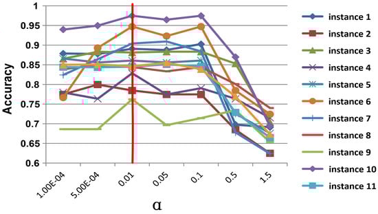
Figure 5.
Parameter Influence on of SCSA on ImageNet dataset. The y-axis represents the classification accuracy of the target domain; the x-axis represents the value range of .
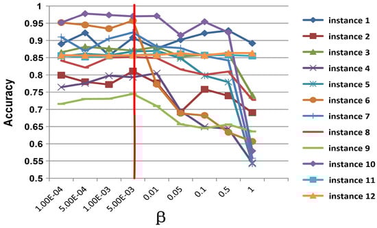
Figure 6.
Parameter influence on of SCSA on ImageNet dataset. The y-axis represents the classification accuracy of the target domain; the x-axis represents the value range of .
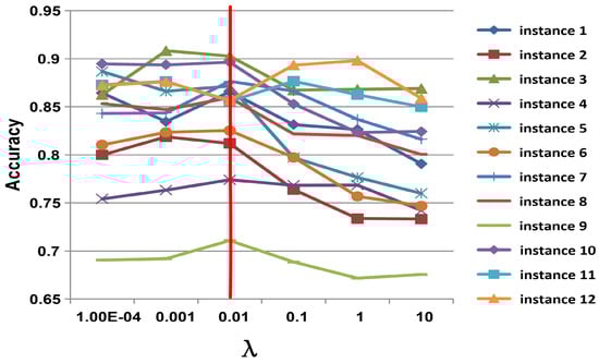
Figure 7.
Parameter influence on of SCSA on ImageNet dataset. The y-axis represents the classification accuracy of the target domain; the x-axis represents the value range of .
6. Conclusions
In this paper, we proposed an unsupervised domain adaptation framework based on a stacked convolution sparse autoencoder, called SCSA. Our method can learn more transferable and discriminative representations across domains. Firstly, the original data is pre-processed by the layer-wise RICA with whitening. Then, the labeled data information in the source domain is encoded via softmax encoder weight regularization in a sparse autoencoder model. Finally, the convolutional kernels are used to reserve the local relevance for learning abstract representations. The proposed method was extensively tested on several datasets and was found to be more effective than state-of-the-art domain adaptation methods. The proposed method was extensively tested on several datasets and an accuracy of up to 89.3% was obtained, outperforming other state-of-the-art autoencoder-based domain adaptation methods, such as SSRLDA.
The designed SCSA is only concerned with the unsupervised domain adaptation of image data and is not concerned with other types of data, such as text data. In the future, we intend to focus on learning better feature representations in text data for unsupervised domain adaptation.
Author Contributions
Conceptualization, Y.Z. and X.W.; methodology, Y.Z. and X.W.; software, Y.Z. and X.Z.; validation, X.Z.; formal analysis, Y.Z.; investigation, X.W.; resources, X.Z.; data curation, X.Z.; writing—original draft preparation, Y.Z. and X.Z.; writing—review and editing, X.W.; visualization, X.W.; supervision, X.W.; project administration, Y.Z. and X.W. All authors have read and agreed to the published version of the manuscript.
Funding
This research is partially supported by the National Natural Science Foundation of China under grants (61906060,62120106008), Yangzhou University Interdisciplinary Research Foundation for Animal Husbandry Discipline of Targeted Support (yzuxk202015,yzuxk202008), the Opening Foundation of Key Laboratory of Huizhou Architecture in Anhui Province under grant HPJZ-2020-02.
Informed Consent Statement
Not applicable.
Conflicts of Interest
The authors declare no conflict of interest. The funders had no role in the design of the study; in the collection, analyses, or interpretation of data.
Appendix A
The aim of the sparse autoencoder is to constrain the neurons in the hidden layers to be inactive most of the time. Given an input set , , and the hidden unit set , , the average activation of the hidden unit can be calculated as (A1):
To ensure that the hidden unit’s activation status is inactive, the constraint is enforced, where p is the sparsity parameter, which is close to zero. The KL divergence method can be used to penalize if it deviates significantly from p, as shown in (A2):
The overall cost function of the sparse auto-encoder can be shown as (A3):
where is defined as (6) and is the hyper-parameter which controls the weight of the sparsity penalty term. Since the term is the average activation of the hidden unit, it also depends on W and b.
References
- Yang, S.; Wang, H.; Zhang, Y.; Li, P.; Zhu, Y.; Hu, X. Semi-supervised representation learning via dual autoencoders for domain adaptation. Knowl.-Based Syst. 2020, 190, 105161. [Google Scholar] [CrossRef]
- Zhu, Y.; Xindong, W.; Li, P.; Zhang, Y.; Hu, X. Transfer learning with deep manifold regularized auto-encoders. Neurocomputing 2019, 369, 145–154. [Google Scholar] [CrossRef]
- Wilson, G.; Cook, D.J. A survey of unsupervised deep domain adaptation. ACM Trans. Intell. Syst. Technol. (TIST) 2020, 11, 1–46. [Google Scholar] [CrossRef] [PubMed]
- Yi, Z.; Hu, X.; Zhang, Y.; Li, P. Transfer Learning with Stacked Reconstruction Independent Component Analysis. Knowl.-Based Syst. 2018, 152, 100–106. [Google Scholar]
- Wang, M.; Deng, W. Deep visual domain adaptation: A survey. Neurocomputing 2018, 312, 135–153. [Google Scholar] [CrossRef]
- You, K.; Long, M.; Cao, Z.; Wang, J.; Jordan, M.I. Universal domain adaptation. In Proceedings of the IEEE/CVF Conference on Computer Vision and Pattern Recognition, Long Beach, CA, USA, 15–20 June 2019; pp. 2720–2729. [Google Scholar]
- Kang, G.; Jiang, L.; Yang, Y.; Hauptmann, A.G. Contrastive Adaptation Network for Unsupervised Domain Adaptation; IEEE: Piscataway, NJ, USA, 2019; pp. 4893–4902. [Google Scholar]
- Deng, J.; Zhang, Z.; Eyben, F.; Schuller, B. Autoencoder-based Unsupervised Domain Adaptation for Speech Emotion Recognition. IEEE Signal Process. Lett. 2014, 21, 1068–1072. [Google Scholar] [CrossRef]
- Ahn, E.; Kumar, A.; Fulham, M.; Feng, D.; Kim, J. Unsupervised Domain Adaptation to Classify Medical Images Using Zero-Bias Convolutional Auto-Encoders and Context-Based Feature Augmentation. IEEE Trans. Med. Imaging 2020, 39, 2385–2394. [Google Scholar] [CrossRef]
- Pan, S.J.; Yang, Q. A survey on transfer learning. IEEE Trans. Knowl. Data Eng. 2009, 22, 1345–1359. [Google Scholar] [CrossRef]
- Feng, S.; Yu, H.; Duarte, M.F. Autoencoder based sample selection for self-taught learning. Knowl.-Based Syst. 2020, 192, 105343. [Google Scholar] [CrossRef]
- Tzeng, E.; Hoffman, J.; Saenko, K.; Darrell, T. Adversarial discriminative domain adaptation. In Proceedings of the IEEE Conference on Computer Vision and Pattern Recognition, Honolulu, HI, USA, 21–26 July 2017; pp. 7167–7176. [Google Scholar]
- Pan, S.J.; Tsang, I.W.; Kwok, J.T.; Yang, Q. Domain adaptation via transfer component analysis. IEEE Trans. Neural Netw. 2011, 22, 199–210. [Google Scholar] [CrossRef]
- Zhuang, F.; Cheng, X.; Luo, P.; Pan, S.J.; He, Q. Supervised representation learning: Transfer learning with deep autoencoders. In Proceedings of the International Joint Conference on Artificial Intelligence, IJCAI, Buenos Aires, Argentina, 25–31 July 2015; pp. 4119–4125. [Google Scholar]
- Yang, S.; Zhang, Y.; Wang, H.; Li, P.; Hu, X. Representation learning via serial robust autoencoder for domain adaptation. Expert Syst. Appl. 2020, 160, 113635. [Google Scholar] [CrossRef]
- Xie, G.S.; Zhang, X.Y.; Yan, S.; Liu, C.L. Hybrid CNN and dictionary-based models for scene recognition and domain adaptation. IEEE Trans. Circuits Syst. Video Technol. 2015, 27, 1263–1274. [Google Scholar] [CrossRef]
- Jaech, A.; Heck, L.; Ostendorf, M. Domain adaptation of recurrent neural networks for natural language understanding. arXiv 2016, arXiv:1604.00117. [Google Scholar]
- Choi, J.; Kim, T.; Kim, C. Self-ensembling with gan-based data augmentation for domain adaptation in semantic segmentation. In Proceedings of the IEEE/CVF International Conference on Computer Vision, Seoul, Republic of Korea, 27 October–2 November 2019; pp. 6830–6840. [Google Scholar]
- Chen, M.; Xu, Z.; Weinberger, K.; Fei, S. Marginalized Denoising Autoencoders for Domain Adaptation. In Proceedings of the ICML, Edinburgh, UK, 26 June– 1 July 2012; pp. 767–774. [Google Scholar]
- Vincent, P.; Larochelle, H.; Lajoie, I.; Bengio, Y.; Manzagol, P.A. Stacked Denoising Autoencoders: Learning Useful Representations in a Deep Network with a Local Denoising Criterion. J. Mach. Learn. Res. 2010, 11, 3371–3408. [Google Scholar]
- Wei, P.; Ke, Y.; Goh, C.K. Deep nonlinear feature coding for unsupervised domain adaptation. In Proceedings of the International Joint Conference on Artificial Intelligence, IJCAI, New York, NY, USA, 9–15 July 2016; pp. 2189–2195. [Google Scholar]
- Zhuang, F.; Cheng, X.; Luo, P.; Pan, S.J.; He, Q. Supervised representation learning with double encoding-layer autoencoder for transfer learning. ACM Trans. Intell. Syst. Technol. (TIST) 2017, 9, 1–17. [Google Scholar] [CrossRef]
- Clinchant, S.; Csurka, G.; Chidlovskii, B. A Domain Adaptation Regularization for Denoising Autoencoders. In Proceedings of the Annual Meeting of the Association for Computational Linguistics (Volume 2: Short Papers), Berlin, Germany, 7–12 August 2016; pp. 26–31. [Google Scholar]
- Yang, S.; Zhang, Y.; Zhu, Y.; Li, P.; Hu, X. Representation learning via serial autoencoders for domain adaptation. Neurocomputing 2019, 351, 1–9. [Google Scholar] [CrossRef]
- Zhu, Y.; Zhou, X.; Li, Y.; Qiang, J.; Yuan, Y. Domain Adaptation with Stacked Convolutional Sparse Autoencoder. In Proceedings of the International Conference on Neural Information Processing, Sanur, Bali, Indonesia, 8–12 December 2021; pp. 685–692. [Google Scholar]
- Ganin, Y.; Lempitsky, V. Unsupervised Domain Adaptation by Backpropagation. In Proceedings of the International Conference on Machine Learning, ICML, Lille France, 6–11 July 2015; pp. 1180–1189. [Google Scholar]
- Sener, O.; Song, H.O.; Saxena, A.; Savarese, S. Learning transferrable representations for unsupervised domain adaptation. Adv. Neural Inf. Process. Syst. 2016, 29, 1–9. [Google Scholar]
- Farahani, A.; Voghoei, S.; Rasheed, K.; Arabnia, H.R. A brief review of domain adaptation. Adv. Data Sci. Inf. Eng. 2021, 877–894. [Google Scholar]
- Zhang, X.; Yu, F.X.; Chang, S.F.; Wang, S. Deep transfer network: Unsupervised domain adaptation. arXiv 2015, arXiv:1503.00591. [Google Scholar]
- Mingsheng, L.; Han, Z.; Jianmin, W.; Jordan, M.I. Unsupervised Domain Adaptation with Residual Transfer Networks. In Proceedings of the Advances in Neural Information Processing Systems, Barcelona, Spain, 5–10 December 2016; Volume 29, pp. 1–9. [Google Scholar]
- Pinheiro, P.O. Unsupervised Domain Adaptation With Similarity Learning. In Proceedings of the IEEE Conference on Computer Vision and Pattern Recognition (CVPR), Salt Lake City, UT, USA, 18–23 June 2018; pp. 8004–8013. [Google Scholar]
- Long, M.; Cao, Z.; Wang, J.; Jordan, M.I. Conditional adversarial domain adaptation. Adv. Neural Inf. Process. Syst. 2018, 31, 1647–1657. [Google Scholar]
- Pei, Z.; Cao, Z.; Long, M.; Wang, J. Multi-adversarial domain adaptation. In Proceedings of the Thirty-Second AAAI Conference on Artificial Intelligence, New Orleans, LA, USA, 2–7 February 2018; pp. 877–894. [Google Scholar]
- Zhang, T.; Wang, D.; Chen, H.; Zeng, Z.; Guo, W.; Miao, C.; Cui, L. BDANN: BERT-based domain adaptation neural network for multi-modal fake news detection. In Proceedings of the 2020 international joint conference on neural networks (IJCNN), Glasgow, UK, 19–24 July 2020; pp. 1–8. [Google Scholar]
- Guo, X.; Li, B.; Yu, H. Improving the Sample Efficiency of Prompt Tuning with Domain Adaptation. arXiv 2022, arXiv:2210.02952. [Google Scholar]
- Chen, Y.; Song, S.; Li, S.; Yang, L.; Wu, C. Domain space transfer extreme learning machine for domain adaptation. IEEE Trans. Cybern. 2019, 49, 1909–1922. [Google Scholar] [CrossRef] [PubMed]
- He, Y.; Tian, Y.; Liu, D. Multi-view transfer learning with privileged learning framework. Neurocomputing 2019, 335, 131–142. [Google Scholar] [CrossRef]
- Chen, M.; Zhao, S.; Liu, H.; Cai, D. Adversarial-Learned Loss for Domain Adaptation. In Proceedings of the AAAI Conference on Artificial Intelligence, New York, NY, USA, 7–12 February 2020; pp. 3521–3528. [Google Scholar]
- Wang, Y.; Qiu, S.; Ma, X.; He, H. A prototype-based SPD matrix network for domain adaptation EEG emotion recognition. Pattern Recognit. 2021, 110, 107626. [Google Scholar] [CrossRef]
- Liu, F.; Lu, J.; Zhang, G. Unsupervised heterogeneous domain adaptation via shared fuzzy equivalence relations. IEEE Trans. Fuzzy Syst. 2018, 26, 3555–3568. [Google Scholar] [CrossRef]
- Yan, Y.; Li, W.; Wu, H.; Min, H.; Tan, M.; Wu, Q. Semi-Supervised Optimal Transport for Heterogeneous Domain Adaptation. In Proceedings of the International Joint Conference on Artificial Intelligence, IJCAI, Stockholm, Sweden, 13–19 July 2018; Volume 7, pp. 2969–2975. [Google Scholar]
- Luo, Y.; Wen, Y.; Liu, T.; Tao, D. Transferring knowledge fragments for learning distance metric from a heterogeneous domain. IEEE Trans. Pattern Anal. Mach. Intell. 2019, 41, 1013–1026. [Google Scholar] [CrossRef]
- Glorot, X.; Bordes, A.; Bengio, Y. Domain adaptation for large-scale sentiment classification: A deep learning approach. In Proceedings of the International Conference on Machine Learning, Bellevue, WA, USA, 28 June–2 July 2011; pp. 513–520. [Google Scholar]
- Nikisins, O.; George, A.; Marcel, S. Domain Adaptation in Multi-Channel Autoencoder based Features for Robust Face Anti-Spoofing. In Proceedings of the 2019 International Conference on Biometrics (ICB), Crete, Greece, 4–7 June 2019; pp. 1–8. [Google Scholar]
- Zhu, Y.; Wu, X.; Li, Y.; Qiang, J.; Yuan, Y. Self-Adaptive Imbalanced Domain Adaptation With Deep Sparse Autoencoder. IEEE Trans. Artif. Intell. 2022, 1–12. [Google Scholar] [CrossRef]
- Oquab, M.; Bottou, L.; Laptev, I.; Sivic, J. Learning and transferring mid-level image representations using convolutional neural networks. In Proceedings of the IEEE Conference on Computer Vision and Pattern Recognition, Columbus, OH, USA, 23–28 June 2014; pp. 1717–1724. [Google Scholar]
- Hoffman, J.; Guadarrama, S.; Tzeng, E.S.; Hu, R.; Donahue, J.; Girshick, R.; Darrell, T.; Saenko, K. LSDA: Large scale detection through adaptation. In Proceedings of the Advances in Neural Information Processing Systems, Montreal, QC, Canada, 8–13 December 2014; pp. 3536–3544. [Google Scholar]
- Girshick, R. Fast R-CNN. In Proceedings of the IEEE Conference on Computer Vision and Pattern Recognition, Boston, MA, USA, 7–12 June 2015; pp. 1440–1448. [Google Scholar]
- Murray, N.; Perronnin, F. Generalized max pooling. In Proceedings of the IEEE Conference on Computer Vision and Pattern Recognition, Columbus, OH, USA, 23–28 June 2014; pp. 2473–2480. [Google Scholar]
- Boureau, Y.L.; Ponce, J.; LeCun, Y. A theoretical analysis of feature pooling in visual recognition. In Proceedings of the ICML, Haifa, Israel, 21–24 June 2010; pp. 111–118. [Google Scholar]
- Li, X.; Armagan, E.; Tomasgard, A.; Barton, P. Stochastic pooling problem for natural gas production network design and operation under uncertainty. AIChE J. 2011, 57, 2120–2135. [Google Scholar] [CrossRef]
- Krizhevsky, A.; Sutskever, I.; Hinton, G.E. ImageNet classification with deep convolutional neural networks. In Proceedings of the ICNIPS, Lake Tahoe, NV, USA, 3–6 December 2012; pp. 1097–1105. [Google Scholar]
- Jin, X.; Zhuang, F.; Xiong, H.; Du, C.; Luo, P.; He, Q. Multi-task Multi-view Learning for Heterogeneous Tasks. In Proceedings of the ACM International Conference on Conference on Information and Knowledge Management, Shanghai, China, 3–7 November 2014; pp. 441–450. [Google Scholar]
- Ben-David, S.; Blitzer, J.; Crammer, K.; Pereira, F. Analysis of representations for domain adaptation. Adv. Neural Inf. Process. Syst. 2007, 19, 137–145. [Google Scholar]


Disclaimer/Publisher’s Note: The statements, opinions and data contained in all publications are solely those of the individual author(s) and contributor(s) and not of MDPI and/or the editor(s). MDPI and/or the editor(s) disclaim responsibility for any injury to people or property resulting from any ideas, methods, instructions or products referred to in the content. |
© 2022 by the authors. Licensee MDPI, Basel, Switzerland. This article is an open access article distributed under the terms and conditions of the Creative Commons Attribution (CC BY) license (https://creativecommons.org/licenses/by/4.0/).