Abstract
Topology optimization is a computationally expensive process, especially when complicated designs are studied, and this is mainly due to its finite element analysis and iterative solvers incorporated into the algorithm. In the current work, we investigated the application of deep learning methods to computationally accelerate topology optimization. We tested and comparatively analyzed three types of improved neural network models using three different structured datasets and achieved satisfactory results that allowed for the generation of topology optimized structures in 2D and 3D domains. The results of the studies show that the improved Res-U-Net and U-Net are reliable and effective methods among deep learning approaches for the computational acceleration of topology optimization problems. Moreover, based on the results, it is evaluated that Res-U-Net gives better results than U-Net for higher iterations. We also showed that the proposed CNN method is highly accurate and required much less training time compared to existing methods.
1. Introduction
1.1. General Knowledge
Topology optimization (TO) is one of the computational tools used for designing lightweight and robust structures and it is well known in many industries. It also indirectly improves the environmental effect of additive manufacturing since less material is used during the 3D printing of structures [1]. Although, when the design of structures is geometrically advanced with multiple initial and boundary conditions, and the computational grid size is fine enough to obtain smoother layouts, the running time of TO significantly increases [2]. Such a computational bottleneck is created mainly due to successive iterations for solving a large system of linear equations obtained from finite element analysis [3].
There are several methods that can be applied to address this issue and these methods are reviewed in our earlier work [4]. Thus, earlier research works are based on high-performance computing that uses multiple CPU and GPU processors, where a computationally expensive portions of algorithms are run in parallel among the cores [5,6]. From the reviewed works, it was clear that CPU- and GPU-based computational accelerations are directly related to the number of elements of FEA (i.e., grid size). Moreover, with the increasing number of processors for parallel computing, higher the time for interprocessor communications, which makes CPU- and GPU-based accelerations time-consuming for problems with a higher number of grid elements [4].
Lately, the application of machine learning (ML) methods for the acceleration of TO run time has gained significant attention. The main reason can be considered as the increasing availability of advanced ML tools, which are also backed up with faster computing hardware [7].
1.2. Related Works in ML
These days, ML methods are being used in various ways to accelerate the running time of TO methods, and here we will review the latest works in this area. The reader should note that the works discussed below are the ones published within the last two years. The reader should refer to our work [4], Section 4.3, to obtain a summarized knowledge of ML-accelerated TO, which are earlier in time than the following works.
Jiang et al. [8] used ML algorithms on so-called moving morphable component (MMC)-based topology optimization. In an MMC-based approach, TO relies on parameter tuning of topological description function (TDF), where the turning is usually carried out manually. To address the latter, an ML-based parameter tuning strategy was proposed, which considers an extra-trees (ET)-based image classifier and particle swarm optimization algorithm. The approach was tested on a cantilever and L-shaped beams and the results are satisfactory.
Qiu et al. [9] developed a deep learning (DL) algorithm for the computational acceleration of TO using a convolutional neural network (CNN) with U-net architecture and recurrent neural network (RNN) with long-short term memory (LSTM) architecture. The trained algorithm was tested for the lightweighting of 2D and 3D cantilever-beam structures. The generated designs showed high accuracy based on a comparative analysis with FEM-based methods. Rade et al. [10] introduced the following two frameworks for TO: density sequence (DS) prediction and coupled density and compliance sequence (CDCS) prediction. The first approach considers a sequential prediction model that allows the transformation of material densities without compliance. In the second method, the authors included intermediate compliance results with the results of improving the efficiency of the compliance predicting surrogate model. Both methods were compared with the baseline approach, so-called direct optimal density (DOD). In case of DS, there are two convolutional neural networks (CNN) are included in it to obtain the final prediction. On the other CDCS is based on three CNNs that iterate while predicting the final optimal topology. The authors demonstrated the better performance of their method by testing it on 2D and 3D structures and comparing the results with a direct density-based approach and SIMP methods.
Yan et al. [11] proposed a new method to predict the results of TO using initial stress learning and DL techniques. A stress matrix was used instead of load cases and boundary conditions. Moreover, the given method doesn’t require repeated iteration and produces real-time results. The algorithm consists of three steps, the first step is the generation of data on the boundary conditions using SIMP (in particular, the main stress matrix at the first iteration, and the result of TO to use as a label); the second step is training the CNN model with the data obtained in step 1; the third step is to test the proposed method for different loading cases. The authors tested the proposed prediction method with the traditional TO method for several examples with a single load. It was observed that the two results are highly approximate.
Another interesting approach of using ML was done by Brown et al. [12] They investigated using reinforcement learning (RL) to automate the designing of 2D topologies. RL is a subset of ML that uses past experience to design an object by removing elements to satisfy compliance minimization objectives. The main advantage of using the RL method is that it does not rely on the pre-creation of the training dataset, to avoid such a time-consuming process. In this method, the algorithm is trained to solve the optimal control problem for the task by receiving feedback or rewards for its work. The algorithm was tested for different load cases, and results showed that it is well adapted to solve the TO problem. The authors showed that the proposed method can optimize 2D objects just as with traditional gradient-based TO methods.
Another interesting approach of using ML was carried out by Brown et al. [12]. They applied deep reinforcement learning to train an agent to design 2D topologies. Compared to other AI and ML methods, reinforcement learning does not need any training data, but relies on the agent that learns to complete a given task or set of tasks within the scope of the interactive environment by providing feedback to the performance of the agent. The reward function is multi-objective and it was built to mimic the multi-objective feature of the compliance minimization in TO. The progressive refinement, from 6 × 6 up to 24 × 24, was conducted using randomly selected loads and bounded elements to train the agent. Once trained, it was tested on other load cases, and compared with gradient-based TO optimizers. The results showed that there is a generalized performance capacity of such apporach, therefore, it is promising for complex tasks of TO.
Sun et al. [13] also proposed a gradient-free method DNN-MFSE, which is a combination of deep neural networks (DNN), and a topology representation model–material-field series expansion (MFSE). The authors concluded that this method indicated better performance compared to other gradient-free methods. Another advantage of the proposed method is the ease of parallel computational implementation since it is a surrogate-based approach. Furthermore, the authors added that this method can be extended to multiphysics problems opening up great opportunities for future studies.
Conditional generative adversarial networks (GANs) are also used to accelerate TO problems [14]. OptiGAN method was proposed by authors for TO of structures. It is a non-iterative method using conditional generative adversarial networks with high accuracy. The proposed method was tested with different datasets, and the average pixel-wise accuracy of the method was estimated to be 83.15%. The authors mentioned that it is a rudimentary phase, and more training needs to be conducted to diversify the spectrum.
Senhora et al. [15] proposed ML-driven framework to accelerate TO. Running time here was reduced by using ML for the sensitivity estimation, thus eliminating FEA to do this procedure. The authors used two-resolution TO: coarse-resolution (for physical information) and fine-resolution (for geometric/topological information) meshes. The information for those two meshes was used as an input for the ML model that predicts the sensitivity, which was then used for a design variables update on the fine-resolution mesh. CNN was used in the ML. Different examples were used to test the proposed method to show its robustness once trained. Moreover, authors mentioned its potential for large-scale problems.
Tan et al. [16] developed surrogate models based on artificial neural networks (ANN) with the purpose of reducing the training time. Particularly, a portion of the training data for full-scale calculations was obtained from coarse-mesh based simulation results. In other words, the proposed ANN-based model, property network, maps the coarse field to corresponding fine field, thus reducing the training time for full-scale TO calculations. Cantilever and L-shaped beams were considered as the test problems. The authors showed comparative analysis for three cases in terms of training cost (i.e., time) with fixed 60 iterations of TO: (i) FEA-based TO, (ii) surrogate model-based TO with fine data and (iii) surrogate model-based TO with hybrid data (coarse and fine mesh based data). Thus, the results showed that the computational time of the latter case (iii) is nearly similar to the case of (i), indicating that the training time of the surrogate model-based TO with hybrid data is compatible with FEA-based TO, while its accuracy is close to the surrogate model-based TO with fine data. Furthermore, the authors further used the trained property network to complete 10 TOs, and the results showed that it is much faster than the conventional FEA-based TO.
1.3. Current Work
In the current work, we propose new ML-based TO methods that allow obtaining of highly accurate results without using computationally intensive FEA studies. In particular, we studied CNN, U-Net and Res-U-Net based ML approaches and tested them for the optimal generation of topology structures. The key scientific design point for the CNN model is to develop an architecture that can be applied for both optimized topology generation in 2D and 3D domains. On the other hand, design points for U-Net and Res-U-Net models reduce not only the computational time to generate optimized topologies, but also the training time, compared to similar models that are used to apply in TO. Thus, three different datasets that contain various optimized topologies for given initial and boundary conditions are used: (i) dataset #1 is generated using SIMP method [17]; (ii) dataset #2 is based on six parameters—volume fraction, displacement boundary condition, load on X axes, load on Y axes, strain energy density and von Mises stress [18]; and (iii) dataset #3, similar to the second one, uses physical fields as input parameters and corresponding output images of optimized topologies [19]. It has been shown that the performance of machine learning models which are based on convolutional mapping (CNN, U-Net, and Res-U-Net) are superior among deep learning algorithms. The performance of the ML algorithms trained using the above-listed datasets are compared in terms of accuracy and timing. According to experimental results, the convolutional mapping is effective not only for image-type data, and also for input data that takes into account the main parameters of the TO problem.
Such ML models with reduced training times and higher accuracies are highly promising in accelerating the computational time of TO problems. Previous models such as TopologyGAN [18] and SILONET [19] require much longer training times per epoch (one complete pass of the ML algorithm through the training data) and larger networks with millions of parameters for accurate results. With the proposed modifications and improvements, the new models compared to their predecessors are much faster, robust, and reliable.
Thus, the current work is structured in the following way: firstly, the brief theory of topology optimization and its computational complexity are introduced. In the main section, the proposed ML methods, including datasets, are considered, which are followed by the description of numerical experiments and results. Finally, conclusive remarks are provided.
2. Topology Optimization Theory
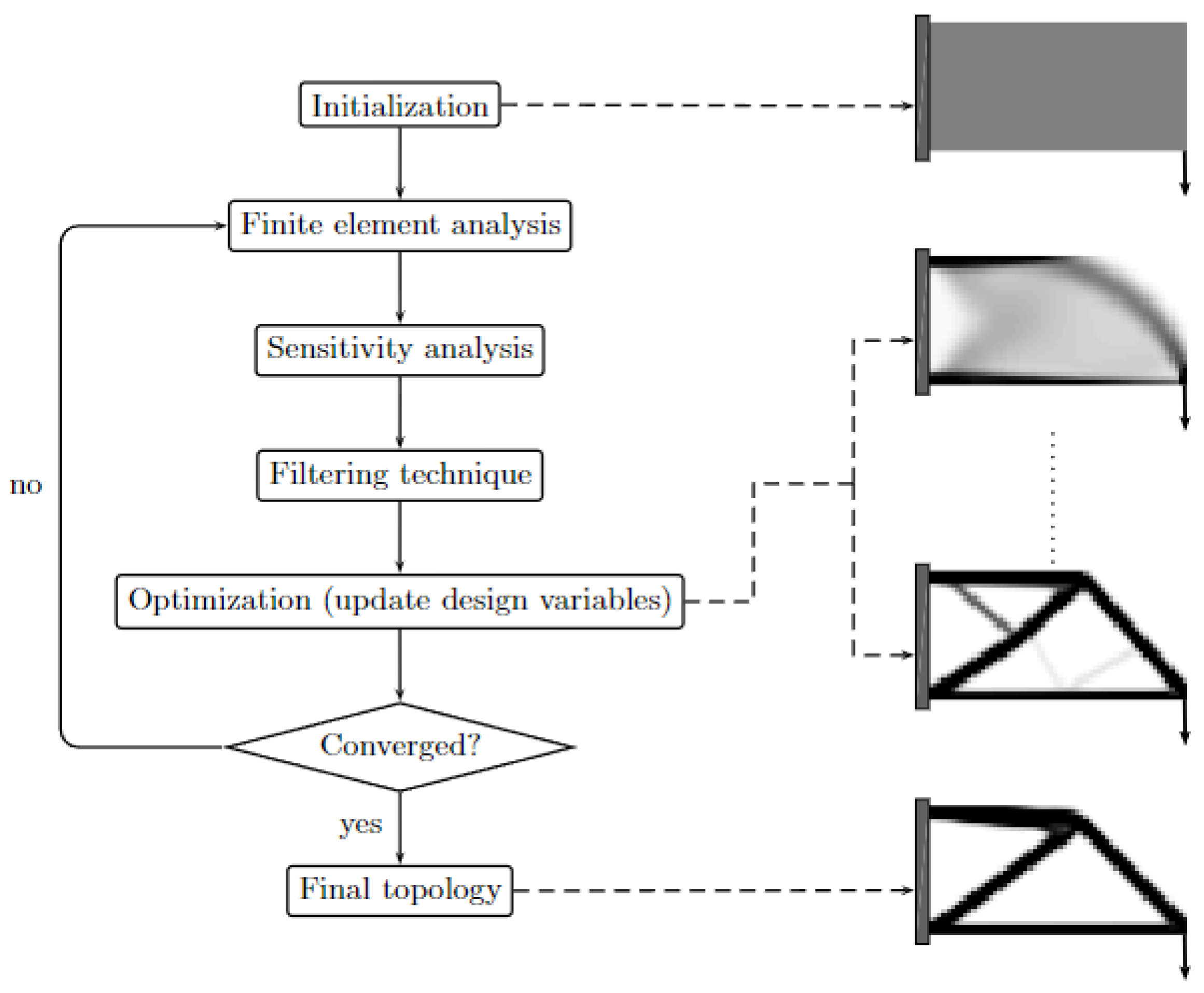
Topology optimization (TO) is a method for optimizing the distribution of material within a given space for a given set of initial and boundary conditions. The method is based on steps of finite element analysis, sensitivity, filtering, optimization, and updating until convergence to the final topology [20]. The overall steps of the TO are shown in Figure 1. Thus, the TO problem can be described as a search for a material distribution that minimizes the objective function F under a volume constraint. The distribution of material is described by a variable density ρ(x), which can take value 0 (emptiness) or 1 (solid material) at any point in the design plane Ω. The optimization problem for state function can be written in mathematical form as given below [20]:
where —volume constraint and —other possible constraints. The first introduced homogenization approach for the topology approach was developed by Bendsøe and Kikuchi [21], which later led to the evolution of other methods.
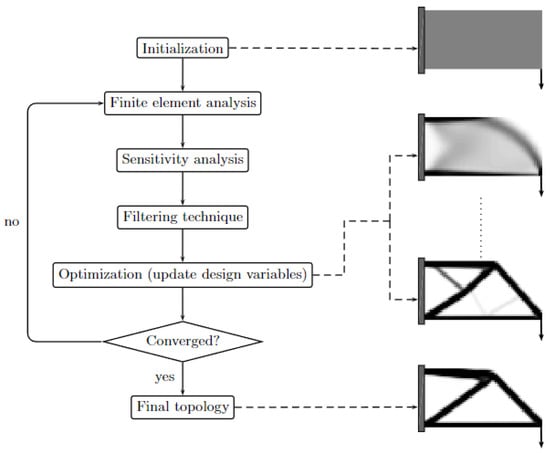
Figure 1.
Schematic illustration of topology optimization steps [3].
So far, several methods have been developed for solving TO problems: the density approach, the level-set approach, the phase field approach, and the discrete approaches [20,22,23]. Among them, the density approach method, and, in particular, the SIMP method (solid isotropic material with penalization) [24] is commonly used by researchers/engineers and it is included in commercial software such as SolidWorks/COMSOL/ANSYS and so on. Thus, a common task of TO, based on the SIMP approach, is to minimize the compliance (i.e., maximize the stiffness) of a given structure under a given mechanical equilibrium, and it can be written as [22]:
where —displacement vector, —force vector, —stiffness matrix, —element displacement, —element stiffness matrix.
The optimization problem can be solved using various iterative methods, such as the optimality criteria (OC) method, the sequential linear programming (SLP) method, or the moving asymptotes (MMA) method [25]. Any of these methods require significant running time. Thus, considering the computational cost of the conventional TO methods, acceleration techniques that permit the obtaining of optimized structures are of interest. Below, we propose ML-based solutions that are reliable, highly accurate, and promising for TO applications.
3. Datasets
We investigated deep learning methods for speeding up the topology optimization (TO) process over three different datasets. These datasets were created by different research groups, and it allows us to compare our results with them accordingly.
3.1. Dataset #1
The first dataset consists of 10,000 synthetic structures created by I. Sosnovic and I. Oseledets [17] using SIMP-based open source topology solver Topy [26]. Pseudo-random problem formulations are used during the dataset generation. For each formulated problem, initial hundred iterations of the standard SIMP method are generated. All problems are based on loads and constraints as described below:
- The number of nodes with fixed x and y translations and the number of loads are sampled from the Poisson distribution [17]:
The nodes for the constraints provided above are sampled from the distribution evaluated on the grid.
- The load values are set to be equal to −1.
- Normal distribution from the equation below was used for the volume fraction sampling.where —mean and —standard deviation.
All generated images are tensors with dimensions equal to 100 × 40 × 40, where 100 is the number of iterations in the standard SIMP approach and 40 × 40 is the dimension of the grid. Thus, two types of inputs are used as shown in Figure 2: (i) density distribution at n-th iteration, and a gradient of n-th and (n − 1)-th iterations. The outputs are optimal layout (i.e., optimal structure).
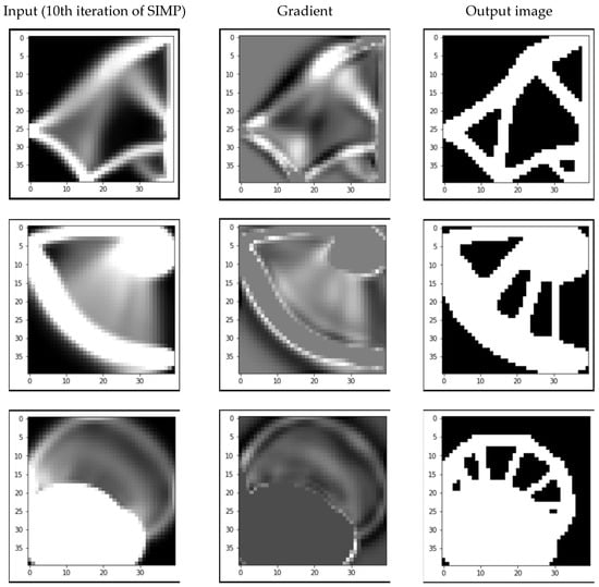
Figure 2.
Images of input, output and gradient of sample in the dataset #1.
3.2. Dataset #2
The second dataset was obtained from the research studies of Nie et al. [18]. The TopologyGAN dataset consists of around 47,000 samples, where each sample has six features with the dimensions of 64 × 128: volume fraction (VF), displacement boundary condition (BC), load on X axes, load on Y axes, strain energy density, von Mises stress described in Figure 2. These features are described below:
- Volume fraction (VF)—desired volume fraction of the output structure. VF value varies in the range starting from 0.3 to 0.5 with the minimum change equal to 0.02. The volume fraction is represented as a matrix completely filled with the desired volume fraction value. All values of this matrix are the same and equal to the VF value, as shown in Figure 3.
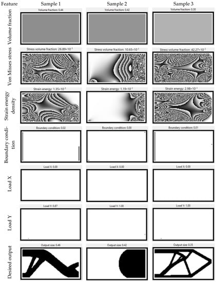 Figure 3. Visual representation of samples of dataset #2.
 - Displacement boundary conditions (BC) are a 2D matrix with the dimension of 64 × 128, which shows the mounting places of the image. Elements of the matrix are described by 0, 1, 2, or 3 numbers, where:
- ○
- 0—unconstrained;
- ○
- 1—ux is equal to zero;
- ○
- 2—uy is equal to zero;
- ○
- 3—both ux and uy are equal to zero;
where ux, uy are displacement vectors on x and y axis. - Load on x axes—is a 2D matrix with the dimension of 64 × 128 filled with zeros and containing at most one float that is less than or equal to one. Load on x axes—external load acting along the x-axis. Only one cell may have a non-zero value which represents external load magnitude and location.
- Load on y axes—2D matrix with the shape 64 × 128 filled with zeros and containing at most one float that is less than or equal to one. Load on y axes—external load acting along the y-axis. Only one cell may have a non-zero value which represents external load magnitude and location.
- Strain energy density—is a physical field applied to the image and calculated using the following equation:
- Von Mises stress is also a physical field applied to the image and calculated using the following equation:where is strain energy density, is the von Mises stress, are components of the stress tensor. All the above-described features are illustrated in Figure 2.
In the current work, we modified input tensors of the TopologyGAN dataset by separating BC features into two feature matrixes in the following way:
- BC on x axes—a matrix for showing points that are fixed on x axes. Basically, it is equal to 1 if ux = 0, otherwise it is 0. Alternatively, it is equal to 1 when the cell is on the original BC, which is equal to either 1 or 3.
- BC on y axes—is a matrix for showing points that are fixed on y axes. Basically, it is equal to 1 if uy = 0, otherwise it is 0. Alternatively, it is equal to 1 when the cell is on the original BC, which is equal to either 2 or 3.
3.3. Dataset #3
The third dataset was generated using the research results by Bielecki et al. [19]. It contains physical fields as an input features and an output image of the desired structure. The authors took the value of optimization parameters as follows: Poisson’s ratio = 0.3; Young’s modulus = 1; minimum Young’s modulus = 10−9; filter radius = 3.2; penalization factor for initial iteration = 2; and penalization factor for later iteration = 8. The structures of the objects are digitalized to 80 × 80.
For 2D Latin hypercube sampling, the volume fraction changes in the range of [0.21–0.99] at 0.01 interval (79 cases), and 5 nodal deflections changes in the range of [0.0–0.5] at 0.1 interval (65 cases). The total training of samples is 614,304 (7776 × 79).
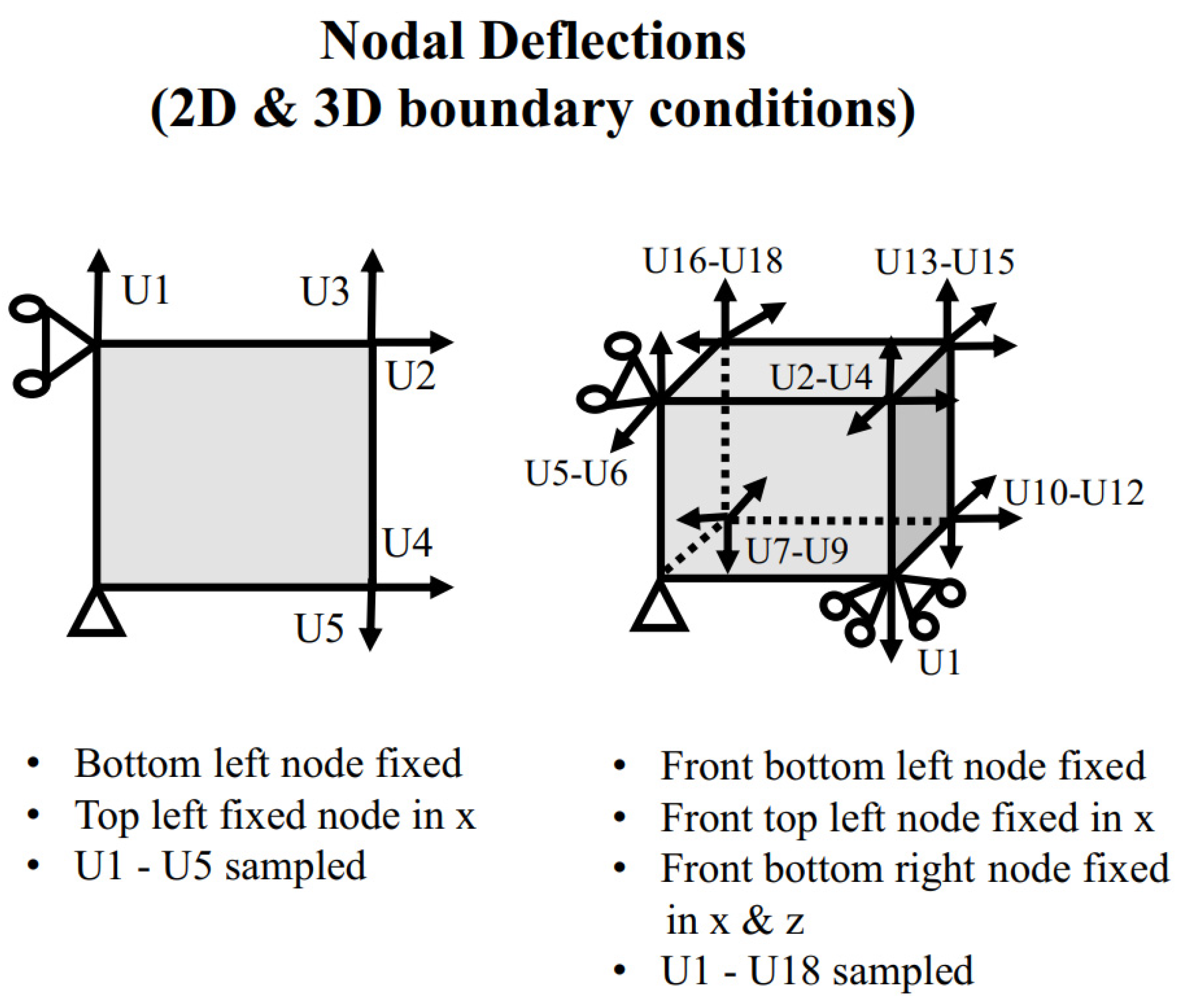
For 3D random sampling, the volume fraction changes in a range of [0.3–0.7] at 0.05 interval (9 cases), and 18 nodal deflections randomly generated in the range of [0.0–0.5] (5000 cases) as shown in Figure 4. Total training of samples are 45,000 (9 × 5000).
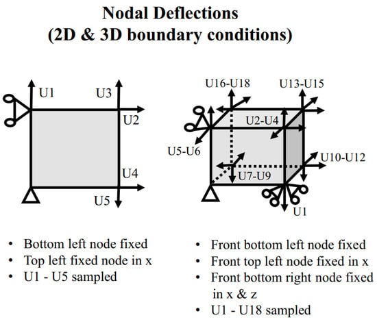
Figure 4.
Description of nodal deflection of 2D and 3D objects [19].
In the paper, inputs of the 2D objects are based on 6 elements {VF, U1:U5}, inputs of the 3D objects are based on 19 elements {VF, U1:18}. We modified the inputs of the objects as follows:
- For 2D objects input vector with [2 × 2 × 3] dimensions:
- For 3D objects input vector with [2 × 2 × 7] dimensions:
4. Model Design
In the work, we investigated the application of deep learning methods such as U-Net, Res-U-Net, and CNN to accelerate the run time of TO methods. For this purpose, we applied U-Net and Res-U-Net to Dataset#1 and Dataset#2 which are based on 2D problems, and CNN to Dataset#3 based on both 2D and 3D structures. Let us describe their architectures separately below.
4.1. CNN
Convolutional neural networks are a special type of artificial neural network that substitutes a commonly used matrix multiplication operation with a mathematical operation called convolution. This operation can be described using Equation (9) mentioned below:
In the scope of this paper, two different CNN models, two and three-dimensional cases have been created. They have the same architecture and differ only in terms of their input and output shapes. For both models, input tensors will pass through two consecutive convolutions, with an initial filter size of thirty-two, and one upsampling layer. This procedure will be performed repeatedly until receiving tensor with a higher shape than the desired one is achieved. Finally, tensors further pass through several convolution layers for obtaining desired output, which is a final optimized layout in our case. Detailed CNN modules are illustrated in Figure 5.
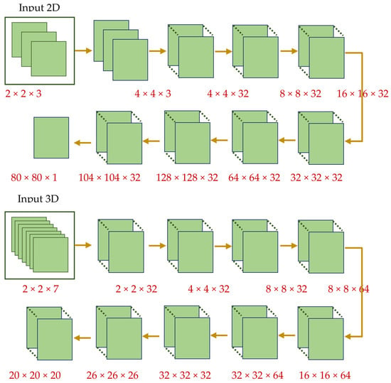
Figure 5.
Visual representation of CNN modules for 2D and 3D objects.
The suggested CNN models are trained on Dataset #3. Inputs of the neural networks are model parameters such as volume fraction and nodal deflections. The output of neural networks is taken to be the optimal structure.
4.2. U-Net
U-Net is a special type of CNN designed for solving image segmentation tasks. It consists of two main stages: contracting and expanding. During the first stage, the model generates N small, filtered versions of the image. In the next stage, all obtained images are upsampled and filtered for receiving the final solution. The solution for this task is the binary image, where 0’s stands for void and 1’s for the material.
U-Net consists of the following layers: convolution, pooling, dropout, and upsampling.
The convolutional layer is a set of learnable filters, which have a small receptive field but extended through the full depth of the input volume. In the scope of our experiment, at each step of the first stage, the total size of the frame is going to be decreased twice, and the number of filters will be increased twice. For the next stage, we apply reverse logic: increase the frame size and decrease the filter size at each step.
Pooling layer: The process of sample-based discretization, where the goal is to down sample the input matrix. In the scope of this experiment, we have used a stride of two (N = M = 2) and the maximum value of each region has been assigned to the resulting matrix:
Dropout (dilution) layer. This is a regularization technique used in artificial neural networks for preventing overfitting. Basically, it sets random values of the dataset to zero and forces machine learning algorithms to learn in a more efficient way.
Upsampling is the process of increasing the width and height of the input matrix by N, M times, correspondingly. In the experiments we have used N = 2, M = 2 and filled the matrix using the following formula:
where is a new matrix and is the initial matrix.
The architecture of the U-Net looks like a symmetrically mirrored convolutional neural network. It consists of two stages: contracting (encoder) and expanding (decoder).
Stage 1: Contracting. This stage follows the regular architecture of CNN. It consists of N repeated applications of two 3 × 3 convolutions each followed by rectified linear unit (ReLU) and a 2 × 2 max pooling operation with stride 2. In our work, the initial number of feature channels is taken to be 8 and the number of channels is increased in a sampling operation.
Stage 2: Expanding. This stage is the reverse of the first one with only one difference: at the beginning of each step, the corresponding feature map is cropped from the contracting path and concatenated with the processed one. The resulting feature map passes through two 3 × 3 convolutions followed by ReLU activation function. Moreover, the generated tensor is upsampled, where the dimensions of the frame are increased twice. In the end, the resulting tensor passes through the last convolutional layer with only one feature channel followed by the sigmoid activation function.
In our experiments, we use the following loss function for the training process:
where, is the value of error and is a predefined coefficient which is equal to 0.5 in the scope of our experiments.
4.3. Res-U-Net
Res-U-Net is an encoder–decoder architecture and refers to deep residual networks and U-Net. It takes advantage of both models, such that residual blocks prevent the vanishing or exploding of gradients in building deeper neural networks, while U-net reconstructs images from generated features.
Similar to U-Net, Res-U-Net has encoding and decoding networks that are connected by a bridge. However, Res-U-Net consists of pre-activated residual blocks instead of simple convolution filters. In the encoder block, neural networks learn the abstract representation of the input image. The bridge is a pre-activated residual block used to stride value 2. The decoder receives features from the bridge and skip connections from encoder blocks to generate better semantic representation.
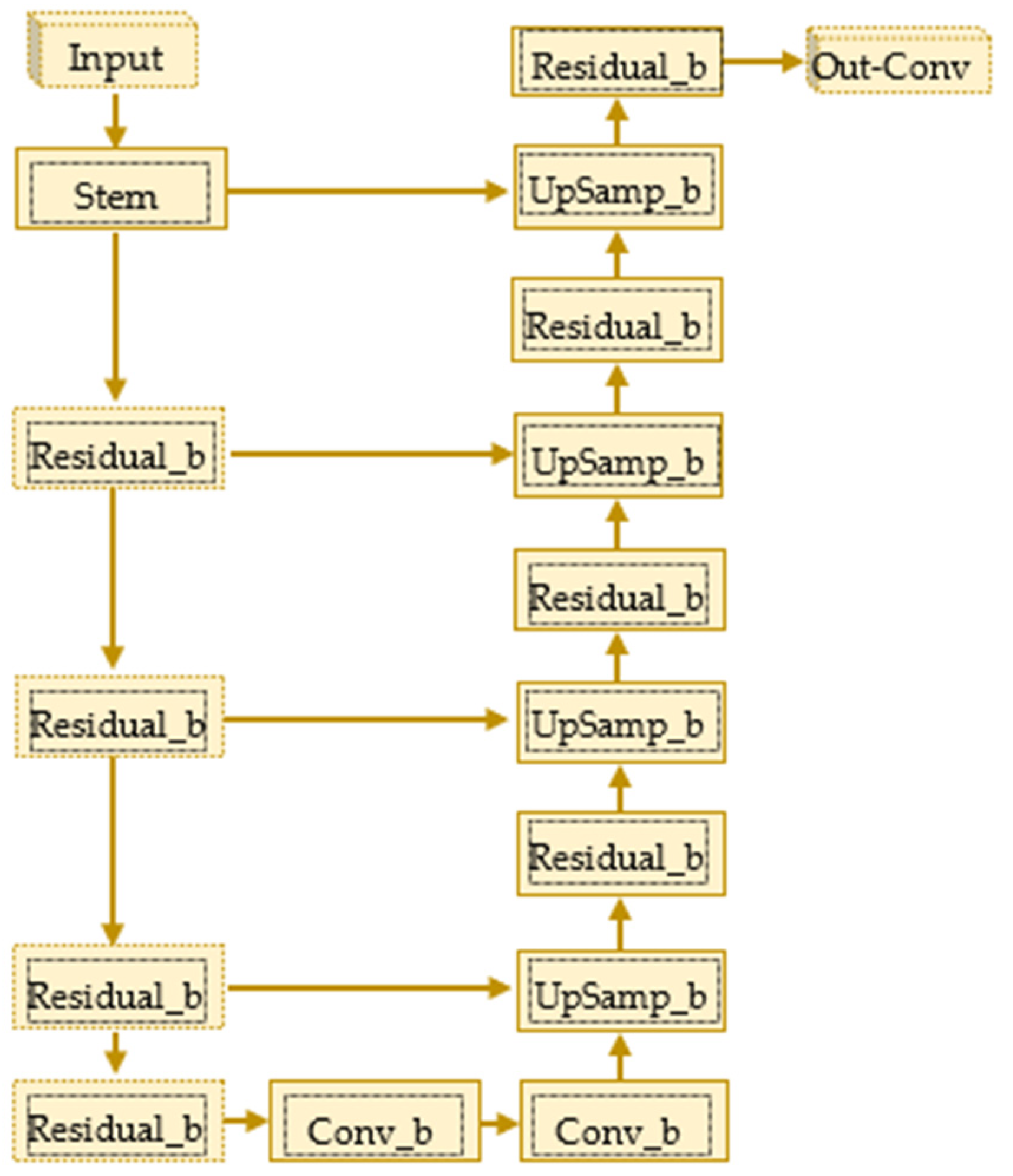
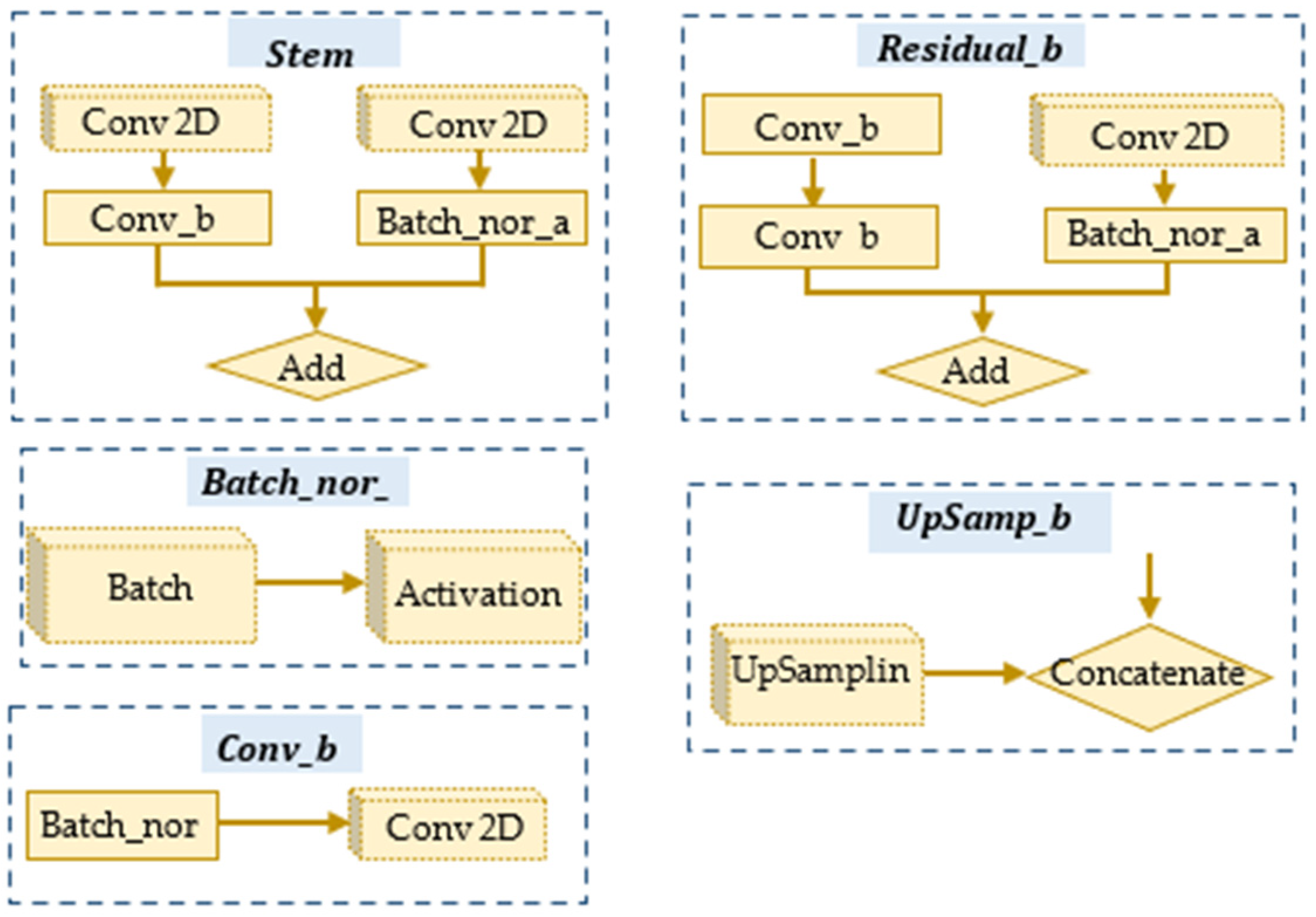
In our experiments, the encoder of the model consists of three residual blocks, and the decoder of model has fur residual blocks. A general description of the proposed Res-U-Net is given in Figure 6. For simplicity, we grouped parts of the networks as Stem, Residual_b, Batch_nor_a, UpSamp_b, and Conv_b as shown in Figure 7.
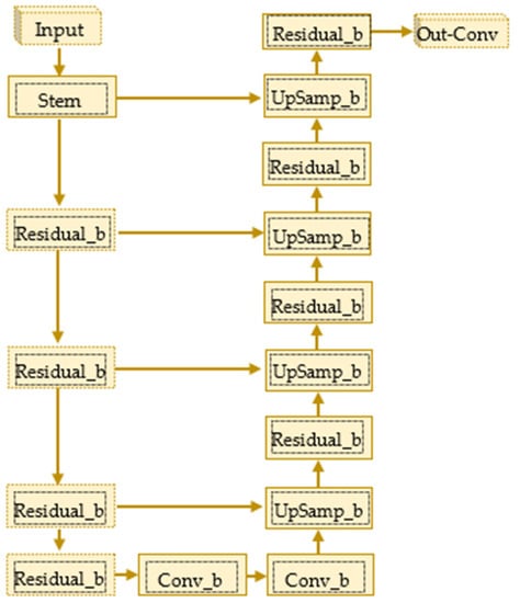
Figure 6.
Visual representation of the proposed Res-U-Net.
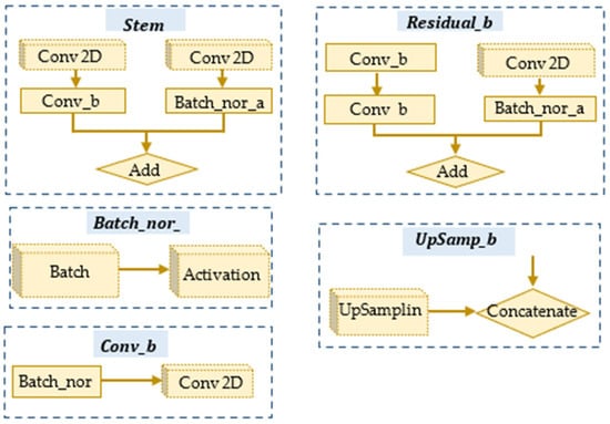
Figure 7.
The main blocks of the Res-U-Net: Stem, Resudual_b, Batch_nor_a, UpSamp_b and Conv_b.
In the experiments, we use mean squared error as the loss function in the training process:
where N is the number of the training samples, is the generated segmentation, is the ground truth.
In both U-Net and Res-U-Net models, we use the same input and output data from Dataset #1 and Dataset #2. The outputs of neural networks are taken to be optimal density distribution (i.e., optimal structure). For Dataset #1, the inputs of the neural networks are intermediate density distributions, which are obtained after n-th iteration of the SIMP model and its gradient. For Dataset #2, inputs of the model are physical parameters as shown in Figure 3.
5. Evaluation Metrics
In the scope of the research work, mean absolute error (MAE), mean square error (MSE), binary accuracy (BA), and intersection over union (IoU) evaluation metrics are used. They measure how much the predicted image differs (MAE, MSE) or similar (BA, IoU) from the desired image.
Mean Absolute Error. The mean absolute error (MAE) is the measure of the error difference between two observations that reflect the same phenomena, and it is written as follows:
Mean Square Error. Mean square error (MSE) is defined as the average of the squares of the errors, or the average squared difference between the estimated and actual values.
Binary accuracy (BA). Exact match or binary accuracy is a metric that compares all pixels of the output image with the target image:
where is the total number of instances of class predicted to belong to class , and is the total number of instances of class .
The intersection over union metric is the percentage of overlapping between the target image and the predicted image.
6. Experiments
6.1. Experiments on Dataset #1
The first experiment contains four different data distributions (DD) as shown in Table 1: Uniform [1–100], Poisson (5), Poisson (10), and Poisson (30). Columns with header 5 to 80 are input iterations for the test model. For example, 5 means that SIMP was used till the 5th iteration and the output of the 5th iteration and the gradient of the 5th iteration are used as inputs of the neural networks. All models were created using TensorFlow API and using Adam optimizer. Authors in [17] used U-Net to train the data in the original paper. Training results depend on hyperparameters and initial values of weights. For a fair comparison of the models, we trained U-net and Res-U-Net on the same initial weights with two different depth values: 3 and 4. According to the experiments, increasing the depth of the model did not play a significant role in obtained results of the correlation between accuracy and iteration. Therefore, we decided to test and compare all experiments with Res-U-Net model with depth 3. Filters of the layers taken as 16, 32, 64, 64, 32, and 16, consequently, in the model.

Table 1.
Binary accuracy score for the U-net and Res-U-Net.
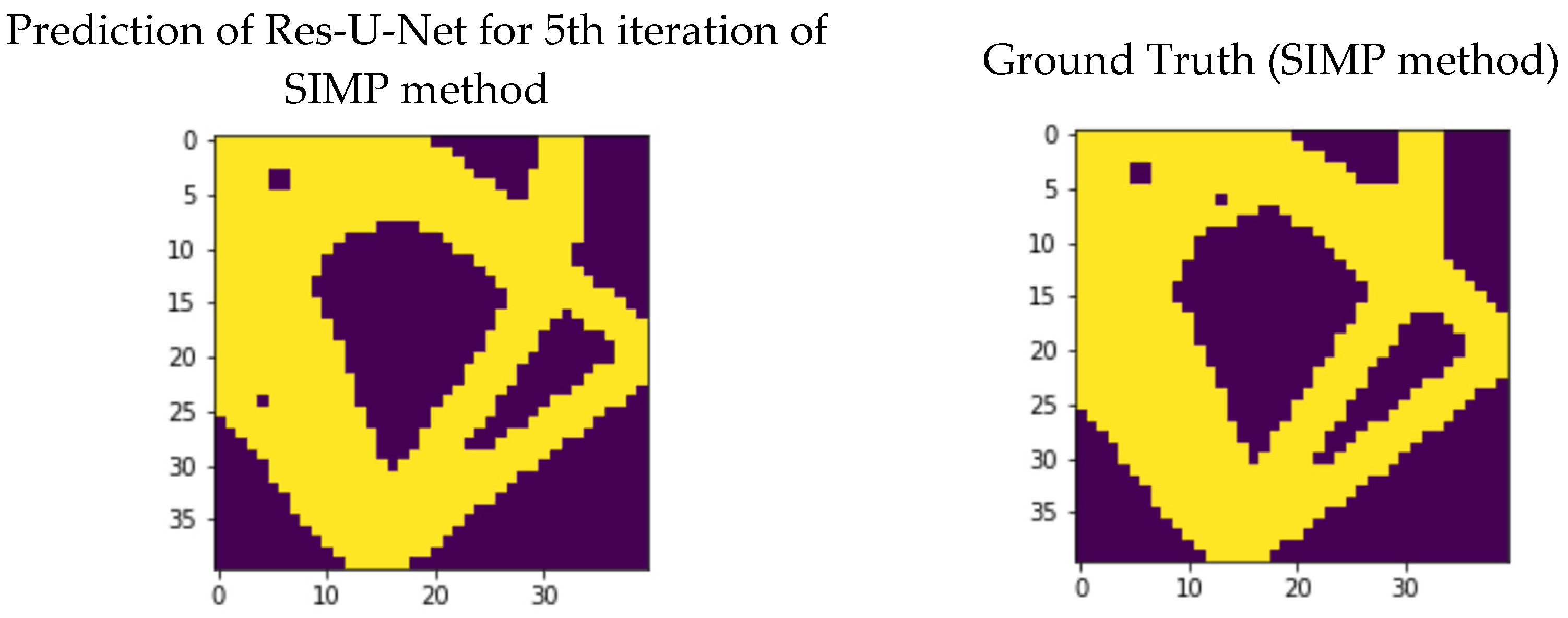
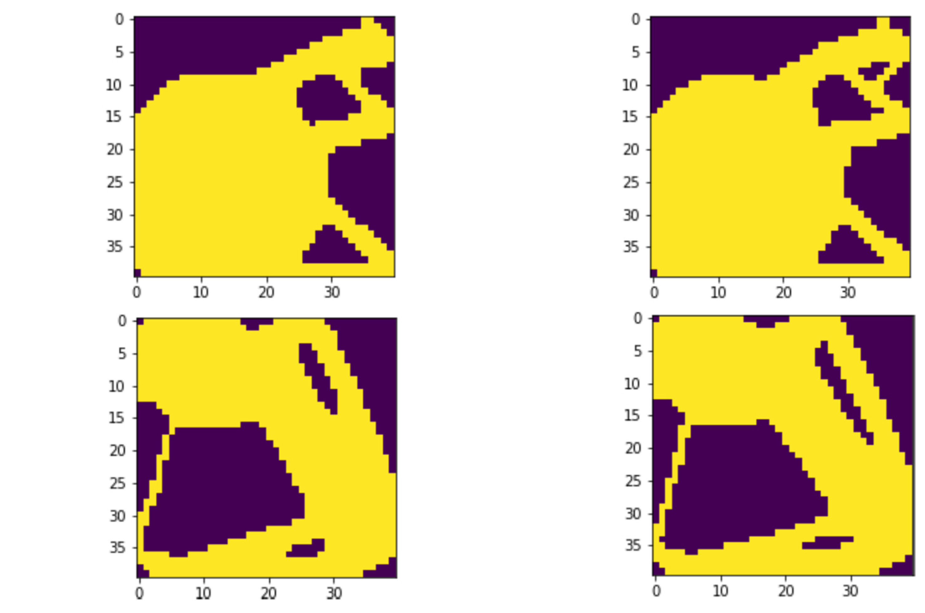
The main evaluation metrics for this experiment are taken to be the binary accuracy score. According to the experiment, U-Net gives better results in lower iteration (5th); however, Res-U-Net is dominant in higher iterations. Although, the accuracy of the Res-U-Net does not significantly deviate from the ground truth even for the predictions in lower iterations and this is shown in Figure 8.

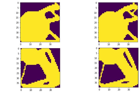
Figure 8.
Outputs of Res-U-Net and ground truth from Dataset #1.
6.2. Experiments on Dataset#2
The authors in [18] applied a TopologyGAN model to train Dataset #2. They used a hybrid generator architecture called U-SE-ResNet in the model. We alternatively modified the input tensors of the dataset by separating BC features into two feature matrixes and applied U-Net and Res-U-Net directly to the modified input data and achieved superior results. The results are provided in Table 2.

Table 2.
Experiments results of 10-fold cross validation accuracy of Res-U-Net and U-Net models.
Similar to [18], we trained the models based on a combination of the parameters of TO: VF—volume fraction, BC—boundary conditions, σ—von Mises Stress, W—strain energy density, L—load on X and Y axes. According to experiment results in Table 3, Res-U-Net with 6 layers with VF, BC, σ, W and L parameters gives better results according to binary and IOU metrics. This means that more accurate results can be achieved using more informative features. The models show superior results with respect to MAE and MSE metrics based on VF, BC, σ, and W parameters.

Table 3.
Dependency between accuracy and features.
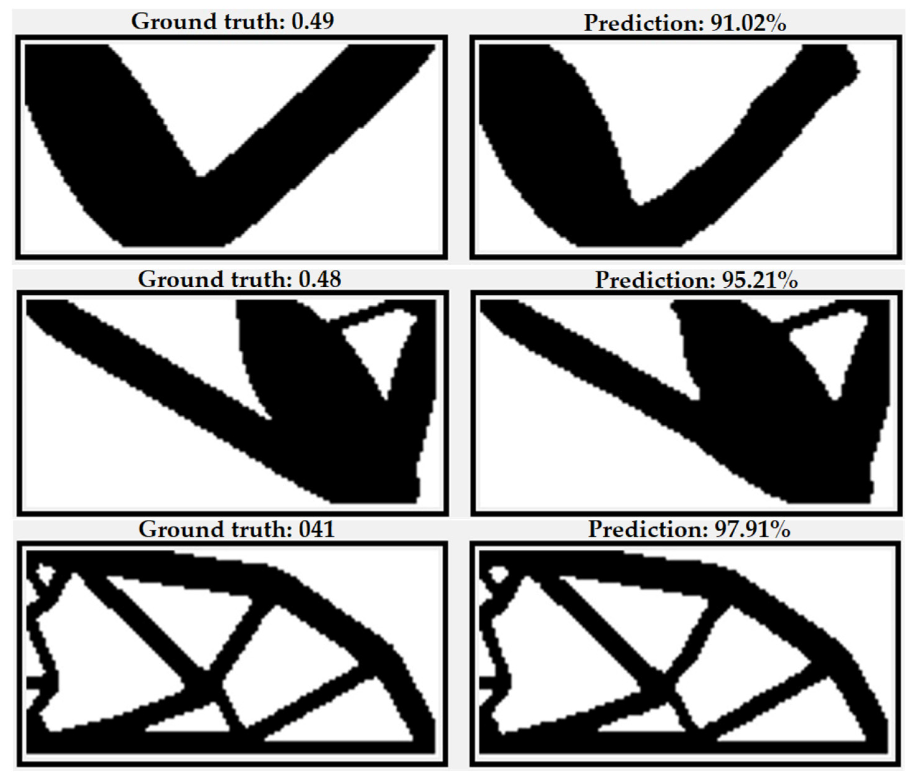
After examining the outputs of the model, it was observed that the main difference occurs in the corners of the structure. Therefore, the geometry of the model is not substantially different from the original. Sometimes it is thinner or thicker than the desired one. Having a thinner structure may decrease the overall strength of the model, which may or may not make the structure fragile. The thicker structure has the same strength but uses more material. We can say that in this case, the best solution is nearly achieved. Several optimized topology layouts of the model training using Dataset #2 are given in Figure 9.
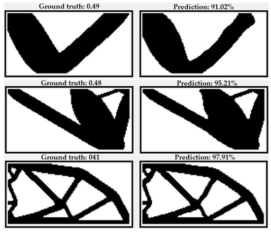
Figure 9.
Outputs of SIMP (left) and Res-U-Net (right) from Dataset #2. In the images of ground truth, 0.49, 048 and 0.41 describes volume fractions.
6.3. Experiments on Dataset #3
Authors of the work [19] applied three stage neural networks to Dataset #3. In the first stage, they used so-called feedforward NN to get a density distribution image. Input and output of the first stage are given to CNN in the second stage. The second stage output is passed through the third stage to obtain globally optimized structures.
In our work, we applied CNN to the same Dataset #3 with modified inputs such as inputs of 2D objects based on 6 elements {VF, U1:U5}, inputs of 3D objects based on 19 elements {VF, U1:18} and achieved 96.67% accuracy for 2D and 93.22% for 3D objects as shown in Table 4. According to the curve of the Loss function of the model, 50 epochs is enough to get the right decision (Figure 10).

Table 4.
Results of the Res-U-Net on the Dataset#3.
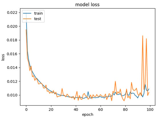
Figure 10.
Illustration of the loss function of model for train and test data.
Generalization is the one of main measures to describe how well the machine learning model has been built. Generalization refers to a model’s ability to adapt properly to new, previously unseen data, obtained from the same distribution as the one used to create the model. One of the gold standards to check generalization ability is to compare test and training accuracies.
Thus, training and testing results of the proposed Res-U-Net are almost the same. The samples for the comparative studies are based on the conventional SIMP model, and the accuracy is 99%, and they are consistently around 99% after 30 iterations. Similar to [18], Dataset #2 is divided into training, validation, and test sets as follows: 4 displacement BCs of the total 42 are randomly selected as the test set. All data samples from the remaining 38 displacement boundary conditions are shuffled and split into training (80%) and validation (20%) sets. Note that the boundary conditions in the test set are not used for training of the neural networks. According to training results, training and validation binary accuracies are around 99%, but the test accuracy is around 90%. The main reason is that training and validation data are from the same distribution (38 scenarios) but test data is taken from another 4 scenarios. For Dataset #2, which has 42 different scenarios, better generalization can be obtained by increasing the variety of the training data (adding additional data with different boundary conditions).
The train, validation, and test binary accuracy are almost same for 2D (~96%), and 3D (~93) on Dataset #3. Better generalization can be obtained by adding different combinations of force values.
To train the suggested models in a similar way, the following software and hardware are required: Python 3.7–3.10; pip version 19.0 or higher for Linux (requires manylinux2010 support) and Windows. pip version 20.3 or higher for macOS.; Windows Native requires Microsoft Visual C++ Redistributable for Visual Studio 2015, 2017 and 2019. The following NVIDIA® software are only required for GPU support.; NVIDIA® GPU drivers version 450.80.02 or higher.; CUDA® Toolkit 11.2.; cuDNN SDK 8.1.0.
7. Conclusions
In the paper, we investigated the possibility of acceleration of standard SIMP approaches using deep learning methods. For this purpose, we tested and comparatively analysed three neural network models on the three different structured datasets introduced by [17,18,19]. The first experiment had a goal to examine the efficiency of boosting SIMP approach by applying Res-U-Net and using different data distributions and different depths of the model. According to the experiment results (Table 1), Res-U-Net gives better results than U-Net for higher iteration, which is considered as a benchmark for Dataset #1 [22]. Additionally, it is defined that increasing the depth of the model by more than three did not play a significant role in the obtained results of the correlation between accuracy and iteration. Moreover, the training model using uniform distribution also has not played a significant role in the accuracy of the resulting model.
The target of the second experiment was to study a deep learning model that can be used as an alternative method to the existing technologies. Initially, there were six different physical parameters that are used for training purposes. In each experiment, some of them were eliminated for understanding their importance and effect on the final result. Von Mises stress, strain energy density, and volume fraction were selected as an initial dataset. Adding boundary conditions as an additional field increased the accuracy of the model. However, the usage of loads for the model slightly decreased the accuracy score. In the second experiment, we modified the input tensors of the dataset by separating boundary conditions (BC) into two feature matrixes in Dataset #2 and applied U-Net and Res-U-Net directly to the modified input data. According to the experiment, MAE = 0.0312 and MSE = 0.0215 are obtained for U-Net, MAE = 0.037 and MSE = 0.48 for Res-U-Net, which are higher than TopologyGAN accuracy presented in the work [24]. Furthermore, TopologyGAN is computationally heavier model than U-Net.
According to experiments with Dataset #1, the proposed Res-U-Net model shows better results in terms of accuracy. But according to the studies with Dataset #2, our U-Net and Res-U-Net models are more effective in terms of timing since they take less than 1 min to train 1 epoch compared to the original TopologyGAN [18] model that takes approximately 15 min to train the 1 epoch. Accuracy results are almost the same in both models.
In the third experiment, we applied CNN to the same Dataset#3 with modified input such as inputs of 2D objects of 6 elements {VF, U1:U5}, inputs of 3D objects consisting of 19 elements {VF, U1:18} and achieved 96.67% accuracy for 2D and 93.22% for 3D objects (Table 4).
In Dataset #3 we used a CNN model, which is comparatively less complex than SILONET [19] in the original paper in terms of depth and model parameters. SILONET consists of two networks that use over 700 million parameters; however, our suggested model uses less than 800 thousand parameters in the training process.
The relationship between the accuracy of the models and number of parameters are given in the Table 5 and Table 6. Due to the shape of the images (40 × 40) in Dataset #1, maximum depth size can be taken as four and it slightly affects the accuracy of the model. On the other hand, images from the Dataset #2 have a bigger shape (64 × 128) which gives us possibilities to increase the depth of the model twice. Such an increase leads to a significant change in accuracy (83.6 vs. 90.07 and 84.32 vs. 89.61).

Table 5.
Binary accuracy score for the Res-U-Net depends on model parameters on the Dataset #1.

Table 6.
Binary accuracy score for the Res-U-Net depends on model parameters on the Dataset #2.
Overall, we defined that Res-U-Net and U-Net are the more reliable and effective methods among deep learning approaches for the computational acceleration of topology optimization problems.
Depending on the boundary condition, the number of elements, volume fraction, minimum radius, penalization, and filter number of iterations required to generate the optimized topology sample varies from tens to thousands of iterations by using SIMP model. For a laptop with Intel Core i7-4510 @2.00 Ghz with up to 2.60 Ghz, the time for one iteration is around 0.88 s. Thus, optimized topology sample generation time can be in the range of tens of seconds to thousands of seconds, respectively. The binary results for the SIMP model estimation were obtained using “ToPy—Topology optimization with Python” code [26]. To obtain better results, a higher number of elements is required, which leads to an increase in sample generation time. In general, it requires a minimum of a few hundred of seconds to generate a fine and detailed optimized topology. According to trained deep learning models, the testing time for the suggested models is less than 1 msec, which is incredibly faster than SIMP model generation. It is worth mentioning that deep learning (DL) requires some time for data preparation and training. Although, optimally designed and trained DL models definitely give advantages in obtaining optimized layouts compared to conventional TO methods.
Thus, improved ML models provide reduced training times and better accuracies for TO problems; therefore, they can be useful for the acceleration of computational time. In the work, we have clearly showed that these new models are highly efficient, robust and reliable compared to their predecessors, TopologyGAN [18] and SILONET [19].
Author Contributions
Conceptualization, S.R. and B.A.; Methodology, S.R. and B.A.; Software, J.R.; Validation, M.N.; Formal analysis, Y.M. and M.N.; Investigation, J.R., S.R., B.A. and Y.M.; Resources, Y.M.; Data curation, M.N.; Writing—original draft, J.R., S.R., B.A. and Y.M.; Visualization, M.N.; Supervision, S.R.; Project administration, B.A. All authors have read and agreed to the published version of the manuscript.
Funding
This work has been supported by the research programme of the Science Committee of the Ministry of Education and Science of the Republic of Kazakhstan (Young Researcher’s Grant No. AP08856141).
Conflicts of Interest
The authors declare no conflict of interest.
References
- Merulla, A.; Gatto, A.; Bassoli, E.; Munteanu, S.I.; Gheorghiu, B.; Pop, M.A.; Bedo, T.; Munteanu, D. Weight reduction by topology optimization of an engine subframe mount, designed for additive manufacturing production. Mater. Today Proc. 2019, 19, 1014–1018. [Google Scholar] [CrossRef]
- Yano, M.; Huang, T.; Zahr, M.J. A globally convergent method to accelerate topology optimization using on-the-fly model reduction. Comput. Methods Appl. Mech. Eng. 2021, 375, 113635. [Google Scholar] [CrossRef]
- Wang, S. Krylov Subscpace Methods for Topology Optimization on Adaptive Meshes. Ph.D. Dissertation, University of Illinois, Champaign, IL, USA, 2007. [Google Scholar]
- Maksum, Y.; Amirli, A.; Amangeldi, A.; Inkarbekov, M.; Ding, Y.; Romagnoli, A.; Rustamov, S.; Akhmetov, B. Computational Acceleration of Topology Optimization Using Parallel Computing and Machine Learning Methods—Analysis of Research Trends. J. Ind. Inf. Integr. 2022, 28, 100352. [Google Scholar] [CrossRef]
- Wang, S.; Sturler, E.; De Paulino, G.H. Large-scale topology optimization using preconditioned Krylov subspace methods with recycling. Int. J. Numer. Methods Eng. 2007, 69, 2441–2468. [Google Scholar] [CrossRef]
- Martínez-Frutos, J.; Herrero-Pérez, D. Large-scale robust topology optimization using multi-GPU systems. Comput Methods Appl. Mech. Eng. 2016, 311, 393–414. [Google Scholar] [CrossRef]
- Dai, W.; Berleant, D. Benchmarking contemporary deep learning hardware and frameworks: A survey of qualitative metrics. In Proceedings of the 2019 IEEE First International Conference on Cognitive Machine Intelligence (CogMI), Los Angeles, CA, USA, 12–14 December 2019; pp. 148–155. [Google Scholar] [CrossRef]
- Jiang, X.; Wang, H.; Li, Y.; Mo, K. Machine Learning based parameter tuning strategy for MMC based topology optimization. Adv. Eng. Softw. 2020, 149, 102841. [Google Scholar] [CrossRef]
- Qiu, C.; Du, S.; Yang, J. A deep learning approach for efficient topology optimization based on the element removal strategy. Mater. Des. 2021, 212, 110179. [Google Scholar] [CrossRef]
- Rade, J.; Balu, A.; Herron, E.; Pathak, J.; Ranade, R.; Sarkar, S.; Krishnamurthy, A. Algorithmically-consistent deep learning frameworks for structural topology optimization. Eng. Appl. Artif. Intell. 2021, 106, 104483. [Google Scholar] [CrossRef]
- Yan, J.; Zhang, Q.; Xu, Q.; Fan, Z.; Li, H.; Sun, W.; Wang, G. Deep learning driven real time topology optimisation based on initial stress learning. Adv. Eng. Inform. 2022, 51, 101472. [Google Scholar] [CrossRef]
- Brown, N.; Garland, A.P.; Fadel, G.M.; Li, G. Deep Reinforcement Learning for Engineering Design Through Topology Optimization of Elementally Discretized Design Domains. Mater. Des. 2022, 218, 110672. [Google Scholar] [CrossRef]
- Sun, Z.; Wang, Y.; Liu, P.; Luo, Y. Topological dimensionality reduction-based machine learning for efficient gradient-free 3D topology optimization. Mater. Des. 2022, 220, 110885. [Google Scholar] [CrossRef]
- Yang, X.; Bao, D.W.; Yan, X. OptiGAN: Topological Optimization in Design Form-Finding with Conditional GANs. In Proceedings of the 27th International Conference of the Association for Computer-Aided Architectural Design Research in Asia (CAADRIA) 2022, Sydney, Australia, 9–15 April 2022. [Google Scholar] [CrossRef]
- Senhora, F.V.; Chi, H.; Zhang, Y.; Mirabella, L.; Tang, T.L.E.; Paulino, G.H. Machine learning for topology optimization: Physics-based learning through an independent training strategy. Comput. Methods Appl. Mech. Eng. 2022, 398, 115116. [Google Scholar] [CrossRef]
- Kai, R.; Chao, T.; Michael, Q.; Wenjing, W. An efficient data generation method for ANN—Based surrogate models. Struct Multidiscip. Optim. 2022, 65, 90. [Google Scholar] [CrossRef]
- Sosnovik, I.; Oseledets, I. Neural networks for topology optimization. Russ. J. Numer. Anal. Math. Model. 2019, 34, 215–223. [Google Scholar] [CrossRef]
- Nie, Z.; Lin, T.; Jiang, H.; Kara, L.B. TopologyGAN: Topology optimization using generative adversarial networks based on physical fields over the initial domain. J. Mech. Des. Trans. ASME 2021, 143, 031715. [Google Scholar] [CrossRef]
- Bielecki, D.; Patel, D.; Rai, R.; Dargush, G.F. Multi-stage deep neural network accelerated topology optimization. Struct. Multidiscip. Optim. 2021, 64, 3473–3487. [Google Scholar] [CrossRef]
- Sigmund, O.; Maute, K. Topology optimization approaches: A comparative review. Struct. Multidiscip. Optim. 2013, 48, 1031–1055. [Google Scholar] [CrossRef]
- Bendsøe, M.P.; Kikuchi, N. Generating optimal topologies in structural design using a homogenization method. Comput. Methods Appl. Mech. Eng. 1988, 71, 197–224. [Google Scholar] [CrossRef]
- Sigmund, O. A 99 line topology optimization code written in matlab. Struct. Multidiscip. Optim. 2001, 21, 120–127. [Google Scholar] [CrossRef]
- Neofytou, A.; Yu, F.; Zhang, L.; Kim, H.A. Level Set Topology Optimization for Fluid-Structure Interactions. In Proceedings of the AIAA SCITECH 2022 Forum, San Diego, CA, USA, 3–7 January 2022; pp. 1–17. [Google Scholar] [CrossRef]
- Rozvany, G.I.N. Aims, scope, methods, history and unified terminology of computer-aided topology optimization in structural mechanics. Struct. Multidiscip. Optim. 2001, 21, 90–108. [Google Scholar] [CrossRef]
- Svanberg, K. The method of moving asymptotes—A new method for structural optimization. Int. J. Numer. Methods Eng. 1987, 24, 359–373. [Google Scholar] [CrossRef]
- Hunter, W. Topy—Topology Optimization with Python 2017. Github. Available online: https://github.com/williamhunter/topy (accessed on 16 October 2022).
Disclaimer/Publisher’s Note: The statements, opinions and data contained in all publications are solely those of the individual author(s) and contributor(s) and not of MDPI and/or the editor(s). MDPI and/or the editor(s) disclaim responsibility for any injury to people or property resulting from any ideas, methods, instructions or products referred to in the content. |
© 2022 by the authors. Licensee MDPI, Basel, Switzerland. This article is an open access article distributed under the terms and conditions of the Creative Commons Attribution (CC BY) license (https://creativecommons.org/licenses/by/4.0/).

