A Lidar-Inertial Navigation System for UAVs in GNSS-Denied Environment with Spatial Grid Structures

Featured Application

The proposed navigation system is suitable for UAV navigation in GNSS-denied environments with spatial grid structures. It can be used for the UAV inventory system of dry coal sheds in thermal power plants, the UAV detection system for anti-corrosion coating of truss structures on high-speed railway platforms, the UAV inspection system for large turbine workshops, and other similar systems.

Abstract

With its fast and accurate position and attitude estimation, the feature-based lidar-inertial odometer is widely used for UAV navigation in GNSS-denied environments. However, the existing algorithms cannot accurately extract the required feature points in the spatial grid structure, resulting in reduced positioning accuracy. To solve this problem, we propose a lidar-inertial navigation system based on grid and shell features in the environment. In this paper, an algorithm for extracting features of the grid and shell is proposed. The extracted features are used to complete the pose (position and orientation) calculation based on the assumption of local collinearity and coplanarity. Compared with the existing lidar navigation system in practical application scenarios, the proposed navigation system can achieve fast and accurate pose estimation of UAV in a GNSS-denied environment full of spatial grid structures.

1. Introduction

Automated intelligent UAVs, which have the ability to autonomously sense the location, have been widely used in inspection, survey, and other tasks in GNSS-denial environments [1,2]. A reliable navigation system [3] is a fundamental guarantee for the safe flight of UAV systems in these environments [4]. Therefore, many lidar-inertial navigation systems have been proposed [5,6,7,8], which calculate the pose using line and plane features. However, the working environment of these navigation systems determines whether they can achieve high-precision UAV pose estimation [9]. The lack of plane and line features in the common spatial grid structure of industrial scenes creates significant challenges for the autonomous navigation system of UAVs.

The critical problem of the autonomous navigation scheme of UAVs based on lidar is the point cloud registration of lidar. This is the process of obtaining the relative pose from the changes in the two frame point clouds of the lidar. A typical method used in this process is the iterative closest point (ICP) method [10]. The ICP method is generally divided into two steps. The first step is to calculate the matching relationship between two scans. The second step is to calculate the optimal transfer matrix to minimize the cost function of the distance between matching points. However, when the point cloud is sparse, accurate matching points cannot be found, and when the point cloud is dense, the matching relationship between points is difficult to calculate in real-time. In order to solve these problems, many ICP variants using higher dimensional information in the environment have been proposed. This method extracts features such as lines, curves, and planes from point clouds [11,12] and constructs cost functions of point-to-line [13], point-to-plane [14], and plane-to-plane [15].

A low drift, real-time lidar navigation system LOAM [16] was first proposed. The front end of this navigation system extracts plane features and corner features. These features form a feature point set. In the feature point set, the UAV pose change is solved by minimizing the cost function of the distance from point-to-line and point-to-plane. Due to this feature-based odometer algorithm, it can be solved in real-time in most airborne computers. Many subsequent navigation systems have been improved on this basis. LIO-SAM [17] presents a factor-graph-based, lidar-inertial, loose-coupling method in the front end. It uses the high-precision position and attitude estimated by the lidar to correct the measurement bias of IMU. It also uses high-frequency IMU measurement to predict the lidar’s motion, providing information for point cloud distortion removal and pose estimation solution. Then F-LOAM [18] improved the lidar navigation system. It constructs a new cost function of point-to-line and point-to-plane matching, which results in a faster and more accurate lidar pose estimation solution.

These navigation systems based on plane and corner features are reliable in most artificial environments. However, there is a significant risk of failure when they work in an environment lacking a clear plane and straight edge, such as woods [19], the moon surface [20], etc. Due to the significant difference in resolution between the horizontal and vertical directions of the surrounding lidar, when the number of feature points is insufficient, it will lead to large errors in motion estimation and failure of system positioning. Spatial grid structures are now widely used in industrial and living scenes, mainly including grid structure and shell structure, because of their light weight, strong shape adaptability, and high structural strength. The lidar navigation system used for UAVs is faced with the above problems when it is applied in GNSS-denied environments full of spatial grid structures [21], such as stadiums, terminals, aircraft hangars, factory workshops, coal sheds, and warehouses. The spatial grid structures in industrial and living scenes are shown in Figure 1. When the UAV works in an environment full of hollowed cylindrical grid structures and curved lattice shell structures above the building, it is difficult for the traditional lidar navigation system to obtain sufficient and stable plane features and corner features. This is very challenging to UAVs using a lidar-based navigation system, which limits the use of UAVs in such an environment. Therefore, seeking to address the problems in applying lidar navigation systems in GNSS-denied environments with spatial grid structures, we propose a lidar-inertial navigation system for UAVs based on grid line features and grid surface features.

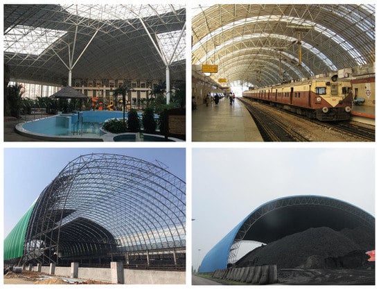
Figure 1. The spatial grid structures in industrial and living scenes.

The main contributions of this study are summarized below:

(1)

Focusing on the spatial grid structure in the GNSS-denied environment, we designed a grid feature-extraction algorithm and a shell feature-extraction algorithm that only use logical judgment.

(2)

We implemented a lidar-inertial navigation system based on the assumption of local collinearity of grid features and local coplanarity of reticulated shell features.

(3)

We experimented with the navigation system in real application scenarios. Experiments undertaken show that, compared with other recently proposed lidar-based UAV navigation systems, the proposed system can achieve faster and more accurate UAV pose estimation in a GNSS-denied environment with spatial grid structures.

The remainder of this paper is organized as follows: The second section introduces the fast extraction algorithm for grid and shell features and the implementation of the navigation system. The third section describes the experiments performed on the navigation system and compares the system with other systems with respect to the following: feature extraction, localization, and mapping. The last section presents the conclusions.

2. Lidar-Inertial Navigation System for UAVs in GNSS-Denied Environment with Spatial Grid Structures

2.1. System Overview

The overall framework of the UAV lidar-inertial navigation system proposed in this paper is shown in Figure 2. The system can be divided into three modules: point cloud extraction and matching, lidar-inertial fusion, and mapping.

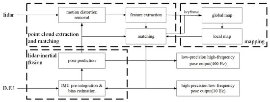
Figure 2. The framework of the proposed navigation system.

The point cloud extraction and matching module receive the point cloud data from the surrounding lidar. Then, the point cloud distortion is removed using the high-frequency pose prediction data of the lidar-inertial fusion module. After the removal of distortion, the features are extracted from the point cloud. Finally, the extracted features are used to match with the local map generated by the mapping module; the high-precision pose is output at a low frequency of 10 Hz.

The lidar-inertial fusion module receives the angular velocity and acceleration data of the IMU and the low-frequency and high-precision pose output by the point cloud extraction and matching module. It pre-integrates the IMU measurement [22] and fuses the above data to achieve loose coupling of lidar-inertial and outputs high-frequency pose prediction. The predicted pose is used for point cloud distortion removal and point cloud matching.

The mapping module receives the matching results from the point cloud matching module and the feature points from the corresponding keyframes. This module uses the above data to build a global map and generates a local map for the point cloud matching module.

2.2. Fast Feature Extraction Algorithm for Spatial Grid Structure

An algorithm is proposed that can quickly and accurately extract grid features and shell features from point clouds collected by lidar in spatial grid structure environments.

Assuming time $t_i$, a frame of point cloud $\widehat{P}$ is obtained by lidar scanning. Because $\widehat{P}$ is usually the point cloud collected by the lidar in continuous time $\left[t_{i-1},t_i\right]$, it is necessary to first remove the original point cloud’s motion distortion to unify all the points in the original point cloud $\widehat{P}$ to time $t_i$. In this way, the measurement error of the sensor can be reduced when solving the pose at time $t_i$ of the navigation system. Since an IMU is used in the navigation system, the method described in [23] is used instead of making the assumption of uniform motion when removing motion distortion:

(1)

Calculate the pose prediction of IMU in the two point cloud frames time interval $\left[t_{i-1},t_i\right]$.

(2)

According to the scanning time of each point in the original point cloud $\widehat{P}$, interpolate the pose transformation of the point to the lidar frame $L_i$ at time $t_i$.

(3)

The points are projected to the lidar frame $L_i$ at time $t_i$ through their pose transformation. The lidar point cloud is recorded from which motion distortion has been removed as $P^{L_i}$.

Next, the features of the spatial grid structures are extracted from the point cloud after motion distortion removal. We first introduce the method of grid feature extraction.

When the UAV is working in an environment full of spatial grid structures, the lidar will detect the environment’s three-dimensional information from the building’s interior. Generally, the space truss structure is closer to the lidar than the shell structure. In the same line of lidar scanning, the points falling on the grid structure and the adjacent points falling on the shell structure produce a “V” shape, as shown in Figure 3.

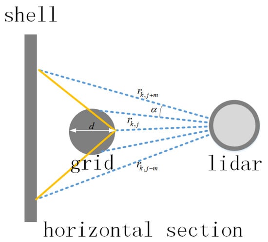
Figure 3. Schematic diagram of the grid feature extraction algorithm. It is a horizontal section view of a spatial grid structure containing vertical truss sections. The blue dotted lines are the lights from the lidar scan points. The yellow lines are an illustration of the “V” shape.

The “V” shape is used to screen the features of the grid on the single-line scanning of the lidar. Denote $P_{k,j}^L$ as the position of the jth point in the lidar frame L of the kth line scan point of a certain frame of lidar. The distance from the point to the center of the lidar is measured as $r_{k,j}$. The characteristic diameter of the steel frame of the spatial grid structure is set as d. The horizontal angular resolution of the lidar is $\alpha$. For each scan point $P_{k,j}^L$, the criteria to be extracted as grid features are shown in Equation (1).

$$\left\{\begin{array}{c}\hfill L_{e\_th}\le r_{k,j+m}-r_{k,j}\le U_{e\_th}\hfill \\ \hfill L_{e\_th}\le r_{k,j-m}-r_{k,j}\le U_{e\_th}\hfill \end{array}\right.$$

(1)

where $L_{e\_th}$, $U_{e\_th}$, and m are all threshold values related to the environment. The expression of m is shown in Equation (2).

$$m=groudup\left(\frac{d}{\alpha r_{k,j}}\right)$$

(2)

where $groudup$ is an operator for upward forensic notation. It is ensured by m that the scan points used to extract the grid features have wholly contained the grid structure and have been irradiated on the shell structure behind.

The shell feature extraction algorithm component in this paper is the same as the extraction method of plane features in the LOAM [16] algorithm. Calculate the average distance $k_{k,j}^L$ from five points before and after a point $P_{k,j}^L$ on each scan line to this point, as shown in Equation (3).

$$k_{k,j}^L=\frac{1}{10·∥P_{k,j}^L∥}\sum _{q\in [-5,5],q\in Z,q\ne 0}∥P_{k,j}^L-P_{k,j+q}^L∥$$

(3)

where $∥P_{k,j}^L∥$ is the distance from point $P_{k,j}^L$ on the line to the center of the lidar, and $∥P_{k,j}^L-P_{k,j+q}^L∥$ is the distance between point $P_{k,j}^L$ and the nearby points $P_{k,j+q}^L$. When $k_{k,j}^L$ is less than the set threshold, it is determined as a plane feature. However, in an environment with space grid structures, multiple consecutive scanning points of the same line of the lidar may fall on the grid simultaneously. In this case, the algorithm will erroneously extract it as a plane feature point. Therefore, we propose a removal algorithm for the false extraction of shell features for space grid structures to turn the plane feature into a shell feature. Its schematic diagram is shown in Figure 4.

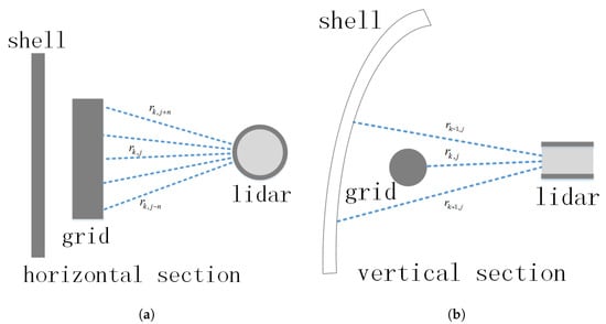
Figure 4. Schematic diagram of the shell feature extraction algorithm. (a) is a horizontal section view of a spatial grid structure containing vertical horizontal sections. (b) is a vertical section view of a spatial grid structure containing vertical horizontal sections. The blue dotted lines are the lights from the lidar scan points.

Figure 4a shows a common situation. In the kth line scan of the lidar, n consecutive scan points before and after the jth scan point fall on the grid. In this case, the point $P_{k,j}^L$ will be judged as a plane feature according to the above single judgment condition. Compared to the LOAM algorithm that only uses a single line scan to extract features, we add the relationship between different line scans to eliminate this erroneous feature extraction. As shown in Figure 4b, the extracted face feature point $P_{k,j}^L$ is compared with the points $P_{k-1,j}^L$ and $P_{k+1,j}^L$ of the same number in the adjacent $k-1$ and $k+1$ lines. If the condition of Equation (4) is satisfied, then $P_{k,j}^L$ is considered to be a point on the shell, which does not need to be eliminated and is recorded as a shell feature. Otherwise, the point is considered to be wrongly extracted and it is eliminated from the plane feature points. In Equation (4), $L_{s\_th}$ and $U_{s\_th}$ are corresponding thresholds.

$$\left\{\begin{array}{c}\hfill L_{s\_th}\le r_{k+1,j}-r_{k,j}\le U_{s\_th}\hfill \\ \hfill L_{s\_th}\le r_{k-1,j}-r_{k,j}\le U_{s\_th}\hfill \end{array}\right.$$

(4)

An example of the extraction of grid and shell features using the proposed method is shown in Figure 5.

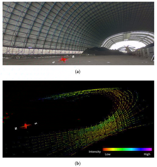
Figure 5. Example of extracting grid features and shell features. (a) shows a GNSS-denied environment with space grid structures, where we operated a UAV with a lidar navigation system flown in. The photo was taken facing north. (b) shows the real-time point cloud collected by the lidar, where the color of the point represents the reflection intensity. (c) shows the grid features and shell features extracted from the point cloud; the grid features are painted in green and the shell features are painted in purple.

2.3. Implementation of the Lidar Navigation System

The proposed lidar-inertial navigation system uses the same fusion framework as LIO-SAM in the front end. The main difference is the design of the lidar odometer part of the navigation system.

To solve the motion of the lidar in a GNSS-denied environment with spatial grid structures, we make certain assumptions about the relationship of the extracted features. The shell feature is assumed to be locally flat. The grid features are assumed to be locally collinear. Then the cost functions of point-to-line and point-to-plane distances are constructed. Compared to the cost function expressions used in LIO-SAM, the proposed methods are compact and easy to construct to solve on SE(3) manifolds.

For the grid feature $P_e^L$, find the five nearest neighbor points corresponding to the feature in the local map $M_{e,local}^N$ composed of grid features. Assume that the five points are collinear. Compute their geometric centers ${\widehat{P}}_e^N$ and the direction vector ${\widehat{n}}_e^N$ of the target line composed of them. The distance $d_e\left(P_e^L\right)$ from the feature point $P_e^L$ to the target line is shown in Equation (5).

$$d_e\left(P_e^L\right)=\alpha ·\left[\left(T_L^N{P}_e^L-{\widehat{P}}_e^N\right)\times {\widehat{n}}_e^N\right]$$

(5)

where $T_L^N$ is the pose transformation matrix representing the lidar in the navigation frame. $\alpha$ is the unit vector of the direction vector from the feature point to the target line. The expression of $\alpha$ is shown in Equation (6).

$$\alpha =\frac{\left(T_L^N{P}_e^L-{\widehat{P}}_e^N\right)\times {\widehat{n}}_e^N}{∥\left(T_L^N{P}_e^L-{\widehat{P}}_e^N\right)\times {\widehat{n}}_e^N∥}$$

(6)

Similarly, the distance $d_s\left(P_s^L\right)$ from the shell feature $P_s^L$ to the target plane is shown in Equation (7).

$$d_s\left(P_s^L\right)=\left(T_L^N{P}_s^L-{\widehat{P}}_s^N\right)\times {\widehat{n}}_s^N$$

(7)

where ${\widehat{P}}_s^N$ is the geometric center of the nearest-neighbor points, which are assumed to be coplanar, corresponding to the shell feature $P_s^L$ in the local map $M_{s,local}^N$ composed of shell features, and ${\widehat{n}}_s^N$ is the normal vector of the target plane.

For all the features, the particular UAV pose at the current moment can be obtained by minimizing the sum of the above cost functions. The output frequency of this pose result is 10 Hz. It is then fused with the IMU using factor graph optimization [24], which is solved by iSAM2 [25].

3. Experiment

3.1. Experimental System Construction

The hardware used in the navigation system experiment included a surround lidar, a six-axis inertial measurement unit, and an onboard computing unit. The surround lidar was VLP-16, with a maximum detection distance of 100 m and an accuracy of 3 cm. It has a field of view angle of 360° horizontally and 30° vertically. During the experiment, the rotational speed was set to 600 rpm, the corresponding horizontal resolution was 0.2°, and the angle between adjacent lines of the 16 scan lines was 2°.

The proposed navigation system is implemented in C++ language. The software was developed based on the ROS architecture and runs on the Ubuntu18.04 operating system. The computing unit used was Intel NUC8 and the CPU was i5-8259U. The navigation system was mounted on a quadrotor UAV and the experiments were carried out in a GNSS-denied environment with space grid structures. The experimental system equipment is shown in Figure 6.

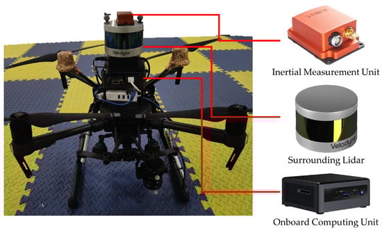
Figure 6. The equipment of the experimental system.

3.2. Experiments and Data Analysis

We chose to test the navigation system in a dry coal shed of the Fengcheng Thermal Power Plant Phase I in Jiangxi Province, China. This is a typical GNSS-denied environment with a spatial grid structure in industrial production. During the experiment, the UAV equipped with the navigation system was manually controlled for flight. Various data were collected and recorded during the experiment. We analyzed the recorded data and compared the proposed navigation system with other systems in terms of the following: feature extraction, localization, and mapping.

3.2.1. Analysis of Feature Extraction

The parameter settings of the feature extraction of the navigation system in the experiment are shown in Table 1.

Table 1. Parameter settings of the feature extraction.

Parameter	${\mathit{L}}_{\mathit{e}\_\mathit{t}\mathit{h}}$	${\mathit{U}}_{\mathit{e}\_\mathit{t}\mathit{h}}$	${\mathit{L}}_{\mathit{s}\_\mathit{t}\mathit{h}}$	${\mathit{U}}_{\mathit{s}\_\mathit{t}\mathit{h}}$	d
Value /m	0.3	6	0.3	6	0.2

The number and total time consumption of feature extraction in each frame of the point cloud are shown in Figure 7. From Figure 7, the total time spent extracting feature points in each point cloud frame showed the same trend as the number of shell features. This implies that the time consumption when extracting features mainly occurred as a result of the extraction of the shell features. It also reflects that the proposed grid feature extraction algorithm, which only uses logical judgment, can perform fast and efficient operations even with limited airborne resources.

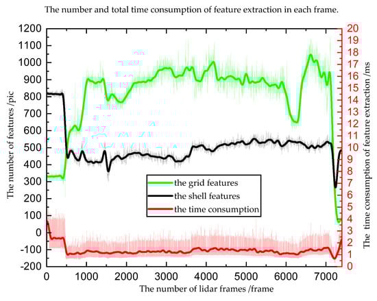
Figure 7. The number and time consumption of feature point extraction.

We analyzed and compared the features extracted by the proposed algorithm and the LOAM algorithm from the spatial grid structure. The features extracted by each algorithm in the low-altitude take-off and landing stage and the high-altitude cruise stage of the UAV are shown in Figure 8. It can be seen from (e) and (f) that, in the low-altitude take-off and landing stage, the LOAM algorithm incorrectly extracted many points belonging to the ground as line features. It can also be seen from (g) and (h) that, in the high-altitude cruise phase, the LOAM algorithm incorrectly extracted the points that fell on the grid as plane features. The incorrect feature extraction introduced significant errors to the localization. In contrast, it can be seen from (a), (b), (c), and (d) that the proposed feature extraction algorithm was able to accurately extract grid and shell features from the surrounding spatial grid structures, regardless of whether the UAV system worked at low altitude or high altitude.

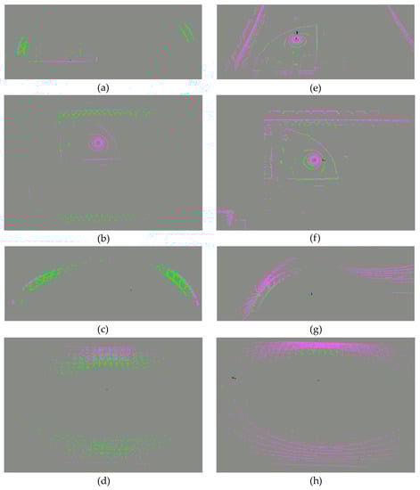
Figure 8. The features extracted by the proposed algorithm and LOAM algorithm. (a,b) are the features extracted by the proposed algorithm for the low-altitude take-off and landing stage of the UAV operations. (c,d) are the features extracted by the proposed algorithm for the high-altitude cruise stage of the UAV operations. In (a–d), we marked the shell feature in pink and the grid feature in green. (e,f) are the features extracted by the LOAM algorithm for the low-altitude take-off and landing stage of the UAV operations. (g,h) are the features extracted by the LOAM algorithm for the high-altitude cruise stage of the UAV operations. In (e–h), we marked plane features in pink and line features in green.

3.2.2. Analysis of Localization

During the experiment, we manually controlled the UAV to fly a complex trajectory in the coal shed until it finally returned to the vicinity of the take-off point. The flight trajectory solved by the proposed navigation system is shown in Figure 9.

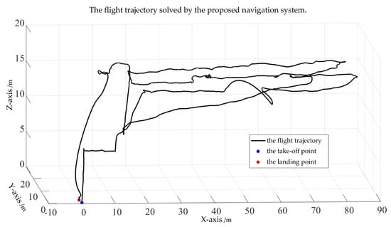
Figure 9. The flight trajectory solved by the proposed navigation system.

The x-axis, y-axis, and z-axis variation curves of the UAV flight trajectory in the coal shed calculated by LOAM, F-LOAM, LIO-SAM, DJI, and the proposed navigation system with time are shown in Figure 10. The UAV flight trajectory and the mapping described in the following subsection are in the navigation frame. We aligned the trajectories computed by the navigation system above. The navigation frame takes the take-off point as its origin. The z-axis is opposite to the direction of gravity and points upwards. The x-axis and the y-axis point to the front and left of the body frame when it is taking off, respectively. In an analysis, we set the local map resolution to remain the same for all navigation systems except DJI. DJI is the positioning system that comes with the drone platform. While working, it fuses data from the IMU, VO, ultrasonic rangefinder, magnetometer, and the barometer. Since DJI does not use lidar, it is only used as an example of the inability of traditional sensor fusion to complete navigation in GNSS-denied environments with spatial grid structures.

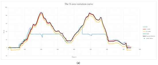
Figure 10. The x-axis, y-axis, and z-axis variation curves of the UAV’s flight trajectory. (a–c) are x-axis, y-axis, and z-axis variation curves with time, respectively.

It can be seen from Figure 10 that the proposed navigation system has higher initial stability than LIO-SAM in the stationary stage before the take-off of the UAV. Except for the height direction, DJI is very different from other systems in other directions. Since the experiment was performed in a GNSS-denied environment, the true value of the UAV pose could not be obtained. Therefore, we compared the error of the UAV landing point solved by each system. In an analysis in this section, we use the offline ICP algorithm to obtain the relative pose between take-off and landing points by matching the point cloud scanned by the lidar during take-off and landing. We take the landing point of the offline solution as the true value and compare the landing point error of each algorithm, as shown in Table 2. It can be seen that the accuracy of the landing point position calculated by the proposed navigation system is significantly better than for the other navigation systems in the x-axis and y-axis directions. It is also close to the best-performing system in the z-axis direction. It should be noted that LIO-SAM uses loop closure detection based on the ICP method in the backend, which is why it has an advantage in the z-direction. The proposed navigation system only acts as a lidar-inertial odometry.

Table 2. Landing point error comparison.

Direction	LIO-SAM	F-LOAM	DJI	Proposed System
X /m	−8.6679	2.1266	−11.8198	0.0550
Y /m	−1.9806	−7.2650	−7.1752	−0.0454
Z /m	0.0399	1.4190	−0.5295	−0.0880

The processing time of a single-scan lidar point cloud of each algorithm is shown in Figure 11. The proposed navigation system converges faster than other algorithms due to the use of better environmental structural constraints in the computation. The average processing time of the proposed system for a single-scan lidar point cloud is under 50 ms.

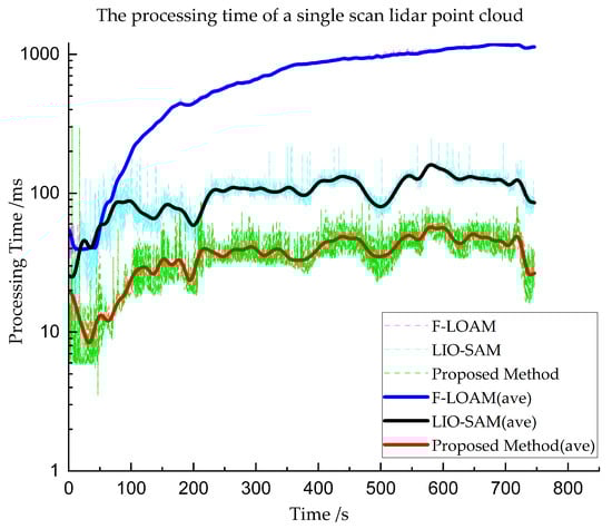
Figure 11. The processing time of a single-scan lidar point cloud.

3.2.3. Analysis of Mapping

We also compared the proposed navigation system with LOAM, F-LOAM, and LIO-SAM in terms of mapping quality. In this subsection, we only show a comparison of the proposed system with LIO-SAM since F-LOAM and LOAM do not produce meaningful point cloud maps. The top view of the point cloud map is shown in Figure 12. The side view of the point cloud map is shown in Figure 13.

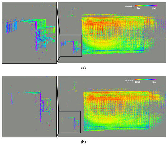
Figure 12. The top view of the point cloud map. (a,b) are the top views of the point cloud maps built by LIO-SAM and the proposed navigation system, respectively.

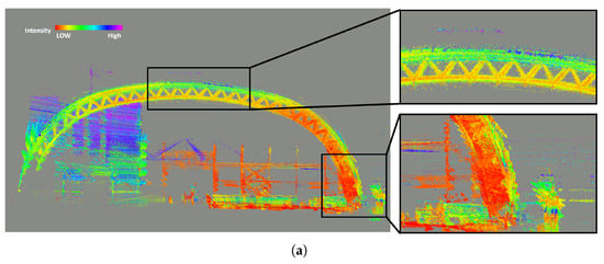
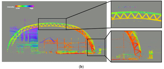
Figure 13. The side view of the point cloud map. (a,b) are the top views of the point cloud maps built by LIO-SAM and the proposed navigation system, respectively.

In Figure 12, we zoom in on the outline of the lower left building in the top view. A lot of “ghosting” appeared in the outline of the building constructed by LIO-SAM. These “ghost images” reflect that LIO-SAM’s estimation of the UAV’s displacement significantly differs from the true displacement in the horizontal direction. In contrast, the proposed navigation system builds a clear outline of the lower left building. This reflects that the proposed navigation system can accurately estimate the displacement in the horizontal direction.

In Figure 13, we zoom in on the bottom support and top of the space grid structure. Compared to LIO-SAM, the proposed navigation system has a more accurate representation of buildings in the constructed map. For example, the thickness of the point cloud on the surface of the shell structure at the top of the coal shed is smaller, and the point cloud at the bottom support better reflects the actual shape of the building structure and wall. This also reflects that the proposed navigation system is very accurate for UAV motion estimation.

4. Conclusions

According to the characteristics of the lidar point cloud in the spatial grid structure, this paper proposes a simple and efficient extraction algorithm for grid features and shell features that only use logical judgment. The algorithm can quickly and accurately extract these two features in the spatial grid structure.

Based on the features extracted from the spatial grid structure, reasonable assumptions are made in this paper. Based on the assumptions, a GNSS-denied environment laser inertial navigation system that adapts to the spatial grid structure is designed and implemented. The navigation system achieves accurate estimation of the UAV’s pose.

In response to the requirements of UAVs for navigation in GNSS-denied environments, we conducted experiments with UAVs equipped with navigation systems in real application scenarios to verify the system’s real-time accuracy with respect to positioning and mapping. By comparing the existing navigation system based on lidar, it was found that the proposed navigation system possesses significant advantages in terms of positioning accuracy, real-time performance, and mapping quality.

References

- Nasrollahi, M.; Bolourian, N.; Zhu, Z.; Hammad, A. Designing LiDAR-equipped UAV platform for structural inspection. In Proceedings of the International Symposium on Automation and Robotics in Construction, Berlin, Germany, 20–25 July 2018; IAARC Publications: Oulu, Finland, 2018; Volume 35. [Google Scholar]
- Rydell, J.; Tulldahl, M.; Bilock, E.; Axelsson, L.; Köhler, P. Autonomous UAV-based forest mapping below the canopy. In Proceedings of the 2020 IEEE/ION Position, Location and Navigation Symposium (PLANS), Portland, OR, USA, 20–23 April 2020. [Google Scholar]
- Dalamagkidis, K.; Valavanis, K.P.; Piegl, L.A. Current Status and Future Perspectives for Unmanned Aircraft System Operations in the US. J. Intell. Robot. Syst. 2008, 52, 313–329. [Google Scholar] [CrossRef]
- Zhou, J.; Kang, Y.; Liu, W. Applications and Development Analysis of Unmanned Aerial Vehicle (UAV) Navigation Technology. J. CAEIT 2015, 10, 274–277+286. [Google Scholar]
- Qin, C.; Ye, H.; Pranata, C.E.; Han, J.; Liu, M. Lins: A lidar-inertial state estimator for robust and efficient navigation. In Proceedings of the 2020 IEEE International Conference on Robotics and Automation (ICRA), Paris, France, 31 May–31 August 2020. [Google Scholar]
- Tagliabue, A.; Tordesillas, J.; Cai, X.; Santamaria-Navarro, A.; How, J.P.; Carlone, L.; Agha-mohammadi, A.-a. LION: Lidar-Inertial observability-aware navigator for Vision-Denied environments. In International Symposium on Experimental Robotics; Springer: Cham, Switzerland, 2020. [Google Scholar]
- Ye, H.; Chen, Y.; Liu, M. Tightly coupled 3d lidar inertial odometry and mapping. In Proceedings of the 2019 International Conference on Robotics and Automation (ICRA), Montreal, QC, Canada, 20–24 May 2019. [Google Scholar]
- Li, K.; Li, M.; Hanebeck, U.D. Towards high-performance solid-state-lidar-inertial odometry and mapping. IEEE Robot. Autom. Lett. 2021, 6, 5167–5174. [Google Scholar] [CrossRef]
- Cadena, C.; Carlone, L.; Carrillo, H.; Latif, Y.; Scaramuzza, D.; Neira, J.; Reid, I.; Leonard, J.J. Past, present, and future of simultaneous localization and mapping: Toward the robust-perception age. IEEE Trans. Robot. 2016, 32, 1309–1332. [Google Scholar] [CrossRef]
- Besl, P.J.; McKay, N.D. Method for registration of 3-D shapes. SPIE 1992, 14, 239–256. [Google Scholar] [CrossRef]
- Pomerleau, F.; Colas, F.; Siegwart, R. A review of point cloud registration algorithms for mobile robot-ics. Found. Trends® Robot. 2015, 4, 1–104. [Google Scholar] [CrossRef]
- Grant, W.S.; Voorhies, R.C.; Itti, L. Finding planes in LiDAR point clouds for real-time registration. In Proceedings of the 2013 IEEE/RSJ International Conference on Intelligent Robots and Systems, Tokyo, Japan, 3–7 November 2013. [Google Scholar]
- Censi, A. An ICP variant using a point-to-line metric. In Proceedings of the 2008 IEEE International Conference on Robotics and Automation, Pasadena, CA, USA, 19–23 May 2008. [Google Scholar]
- Chen, Y.; Medioni, G. Object modelling by registration of multiple range images. Image Vis. Comput. 1992, 10, 145–155. [Google Scholar] [CrossRef]
- Segal, A.; Haehnel, D.; Thrun, S. Generalized-icp. In Robotics: Science and Systems; MIT Press: Cambridge, MA, USA, 2009; Volume 2, p. 435. [Google Scholar]
- Zhang, J.; Singh, S. LOAM: Lidar odometry and mapping in real-time. In Proceedings of the Robotics: Science and Systems, Rome, Italy, 13–15 July 2015; Volume 2, pp. 1–9. [Google Scholar]
- Shan, T.; Englot, B.; Meyers, D.; Wang, W.; Ratti, C.; Rus, D. Lio-sam: Tightly-coupled lidar inertial odometry via smoothing and mapping. In Proceedings of the 2020 IEEE/RSJ International Conference on Intelligent Robots and Systems (IROS), Las Vegas, NV, USA, 25–29 October 2020. [Google Scholar]
- Wang, H.; Wang, C.; Chen, C.L.; Xie, L. F-loam: Fast lidar odometry and mapping. In Proceedings of the 2021 IEEE/RSJ International Conference on Intelligent Robots and Systems (IROS), Prague, Czech Republic, 27 September 27–1 October 2021. [Google Scholar]
- Chen, S.W.; Nardari, G.V.; Lee, E.S.; Qu, C.; Liu, X.; Romero, R.A.F.; Kumar, V. Sloam: Semantic lidar odometry and mapping for forest inventory. IEEE Robot. Autom. Lett. 2020, 5, 612–619. [Google Scholar] [CrossRef]
- Shang, T.; Wang, J.; Dong, L.; Chen, W. 3D lidar SLAM technology in lunar environ-ment. Acta Aeronaut. Astronaut. Sin. 2021, 42, 524166. [Google Scholar]
- Dong, S.L.; Zhao, Y. Discussion on types and classifications of spatial structures. China Civ. Eng. J. 2004, 1, 7–12. [Google Scholar]
- Forster, C.; Carlone, L.; Dellaert, F.; Scaramuzza, D. On-Manifold Preintegration for Real-Time Visual–Inertial Odometry. IEEE Trans. Robot. 2017, 33, 1–21. [Google Scholar] [CrossRef]
- Xu, W.; Zhang, F. Fast-lio: A fast, robust lidar-inertial odometry package by tightly-coupled iterated kalman filter. IEEE Robot. Autom. Lett. 2021, 6, 3317–3324. [Google Scholar] [CrossRef]
- Frank, D.; Michael, K. Factor Graphs for Robot Perception. Found. Trends Robot. 2017, 6, 1–139. [Google Scholar]
- Kaess, M.; Johannsson, H.; Roberts, R.; Ila, V.; Leonard, J.J.; Dellaert, F. iSAM2: Incremental smoothing and mapping using the Bayes tree. Int. J. Robot. Res. 2012, 32, 216–235. [Google Scholar] [CrossRef]
Disclaimer/Publisher’s Note: The statements, opinions and data contained in all publications are solely those of the individual author(s) and contributor(s) and not of MDPI and/or the editor(s). MDPI and/or the editor(s) disclaim responsibility for any injury to people or property resulting from any ideas, methods, instructions or products referred to in the content. |
© 2022 by the authors. Licensee MDPI, Basel, Switzerland. This article is an open access article distributed under the terms and conditions of the Creative Commons Attribution (CC BY) license (https://creativecommons.org/licenses/by/4.0/).