Abstract
Ginseng is a perennial herbaceous plant that has been widely consumed for medicinal and dietary purposes since ancient times. Ginseng plants require shade and cool temperatures for better growth; climate warming and rising heat waves have a negative impact on the plants’ productivity and yield quality. Since Republic of Korea’s temperature is increasing beyond normal expectations and is seriously threatening ginseng plants, an early-stage non-destructive diagnosis of stressed ginseng plants is essential before symptomatic manifestation to produce high-quality ginseng roots. This study demonstrated the potential of fluorescence hyperspectral imaging to achieve the early high-throughput detection and prediction of chlorophyll composition in four varieties of heat-stressed ginseng plants: Chunpoong, Jakyeong, Sunil, and Sunmyoung. Hyperspectral imaging data of 80 plants from these four varieties (temperature-sensitive and temperature-resistant) were acquired before and after exposing the plants to heat stress. Additionally, a SPAD-502 meter was used for the non-destructive measurement of the greenness level. In accordance, the mean spectral data of each leaf were extracted from the region of interest (ROI). Analysis of variance (ANOVA) was applied for the discrimination of heat-stressed plants, which was performed with 96% accuracy. Accordingly, the extracted spectral data were used to develop a partial least squares regression (PLSR) model combined with multiple preprocessing techniques for predicting greenness composition in ginseng plants that significantly correlates with chlorophyll concentration. The results obtained from PLSR analysis demonstrated higher determination coefficients of R2val = 0.90, and a root mean square error (RMSE) of 3.59%. Furthermore, five proposed bands (683 nm, 688 nm, 703 nm, 731 nm, and 745 nm) by stepwise regression (SR) were developed into a PLSR model, and the model coefficients were used to create a greenness-level concentration in images that showed differences between the control and heat-stressed plants for all varieties.
Keywords:
plant phenotyping; ANOVA; band selection; chlorophyll; band ratio image; SPAD readings; PLSR; chemical image 1. Introduction
Ginseng plants are long-lived and slow-growing species that take four to six years for optimal root growth [1]. Ginseng has been consumed for centuries in east Asia due to its health benefits [2]. Disregarding the roots, the aerial parts, including leaves and berries, are increasingly supplemented as food for high ginsenosides and phenolic compositions (p-coumaric acid, cinnamic acid, and syringaresinol) [1]. Along the life cycle, ginseng plants are constantly exposed to extreme stress conditions, with significant concerns related to the projected global temperature increase of 2 °C by 2050 [3], since ginseng plants are susceptible to high temperatures [4], and their photosynthetic efficiency declines starting at 35 °C (48 h) [5]. Several studies have reported the adverse impact of temperature on ginseng plants. For example, subjecting ginseng to high temperatures has been shown to reduce plant and root growth, leaf size, and 29–59% of primary and secondary roots [6]. Additionally, based on reports of destructive methods [5,7,8,9] high-temperature propositional impacts on medicinal compounds of the roots, for instance, cause its ginsenoside content to drop due to a decrease in photosynthesis and protein compositions in leaves [5,9], which causing to damage plants growth and development [10].
Due to ginseng plants’ sensitivity to environmental changes, ginseng grown under an artificial shade has illustrated a higher market value than that grown under direct lighting, as the former crop physically appears smooth, fat, and cream-colored and has few rings on its roots [11]. According to the reported studies, the environment directly affects ginseng’s market value and functional food composition [12]. Therefore, the early diagnosis of biotic and abiotic stress has become extremely important for increasing agriculture productivity and crop quality.
Moreover, perennial plants acquire various physiological and morphological characteristics in their life cycles. Therefore, the quality inspection of plants has become increasingly important. For example, in leaves with high levels of ginsenoside in one-year-old ginseng plants [13], exposure to heat stress was found to reduce the ginsenoside composition [7]. Ginsenoside has various medical applications, such as inhibiting reactions, antiaging, cancer treatment, and other health benefits [14]. Moreover, heat stress impacting the molecular composition of ginseng plants has been reported [9] under differential gene expression in two varieties, which presented significant decreases in chlorophyll (a and b) binding protein, fatty acids, cytochrome, and photosynthesis mechanisms. These studies have contributed significantly to ginseng plants’ physiological, morphological, and biochemical inspection. However, these methods involve destructive approaches that require time and intense labor. Thus, these methods can only be used by specialists.
Advances in imaging technologies offer opportunities for the non-destructive screening of plants’ physiological, biochemical, and morphological characteristics [15]. Non-destructive visualization of plants’ status in early stages will help to minimize non-optimal negative impacts and increase crop yield and quality, in addition to helping create better farm management practices and input efforts. Responding to non-optimal conditions is essential for increasing plants’ nutrition status to avoid devastating consequences for high-quality crop production [16]. For example, the early detection of spotted wilt virus infection in tomatoes was realized using hyperspectral imaging (HSI) [17]. In other studies, a multispectral sensor was used to detect gray mold on tomato leaves [18] and in the early diagnosis of water deficiency in maize plants using HSI [19]. Moreover, near-infrared spectroscopy (NIRS) was used to monitor spinach plant texture and other quality assessments [20]. Furthermore, digital imaging, chlorophyll fluorescence, and visible NIRS were used to monitor bell pepper fruits’ ripening stages [21]. Thermal imaging, which provides temperature information related to plant status [15,22] through long-wave infrared spectra coupled with stereo visible light imaging, was applied to detect diseased tomato plants [23]. Additionally, the early diagnosis of plants based on morphological features has been widely used in color imaging in combination with machine learning and deep learning analysis. For example, digital images were used for early water stress detection in maize plants [24], automated high throughput systems were developed for the evaluation of salt tolerance in soybean plants [25], and a convolution neural network (CNN) was used for the real-time detection of apple leaf disease and identification of Arabica and Robusta coffee plants [26]. Moreover, several spectroscopic and imaging techniques have been used to assess plants’ biotic and abiotic stress detection. Among the non-destructive technologies, HSI combined with chemometrics has been widely used to inspect the phenotypic status of plants.
The main advantage of HSI technology is that it provides spatial and chemical information about a scene/subject beyond the range of human-eye visualization (700 nm). For example, HSI has been used for water stress detection in apple trees [27], early-stage detection of drought stress in Arabidopsis Thaliana plants [28], and the early detection of tomato-spotted wilt virus [29]. In addition, fluorescence HSI is used widely for monitoring plant states and in phenotypic response analysis. FL-HSI was used for drought stress inspection of soybean plants over different treatments [30] and for detecting and quantifying the Pseudomonas Cichorii pathogen in tomato plants [31]. Additionally, hyperspectral chlorophyll fluorescence imaging was used for the early detection of diseases in wheat plants [32], the visualization of infected grapevine leaves associated with leafroll virus and its effects on the photosynthetic of plants [33], the detection of heavy metal effects on plants’ productivity, and the photosynthetic reactions of plants exposed to heavy thallium [34].
Furthermore, advances in hyperspectral imaging technologies are employed to assess solar-induced fluorescence (SIF) for the prediction of the photosynthesis properties of plants. Hyperspectral imaging systems allow for simultaneous and accurate assessment of the SIF emission in plant leaves, which provides a visual representation of physiological changes caused by the photosynthetic activities of the plants in the early stage. For instance, water stress in sugar beet was detected based on the S.I.F. using hyperspectral imaging [35], irrigation deficiency in orange (Citrus sinensis L. cv. Powell) field was monitored [36], and another study assessing forest plants’ health in early stages used hyperspectral imaging for the extraction of SIF [37], and apple tree volume mapping [38]. Since crops’ photosynthetic activities directly influence the physiological changes in plants, further research needs to investigate the involved mechanisms.
In this study, we explored the potential of line-scan fluorescence HSI to detect heat-stressed ginseng plants in the early stages. In a fluorescence illumination system, the photoreactive components of materials must absorb light energy in a particular wavelength to emit the absorbed light. Different objects exhibit different reactions upon exposure to light (absorbing, scattering, or emitting light or any other combination). According to previous studies, fluorescence has been widely applied in agriculture for different purposes, indicating that plants’ compounds are susceptible to releasing absorbed energy from fluorescence. The emission wavelength and intensity are influenced by excitation states, power, and exposure. Ultraviolet or blue illumination is a vital tool for enabling fluorescence applications to assess the chlorophyll composition in plants under stress conditions, in which the ultraviolet excitation radiation generates two broad spectra emissions: blue-green at a range between 400–600 nm, and red and far-red at 600–750 nm [39]. Since the responses of plants’ fluorescence characteristics vary depending on the composition of the leaves, it is essential to identify the samples’ optimal excitation and emission wavelengths. However, fluorescence-based systems suffer from the limitations of acquiring data under dark conditions [40]. Thus, it is recommended that field-based measurement data acquisition should be performed at night [41,42]. The overall objective of this study was to investigate the potential fluorescence HSI for the early detection of stressed ginseng plants—specifically, (i) to develop fluorescence HSI for the prediction of heat-stressed ginseng plants based on measured SPAD greenness quantity, (ii) to extract the spectral information from plants and define the optimal wavebands for the further processing of HSI data based on the F-values computed via analysis of variance (ANOVA), and (iii) to visualize and predict chlorophyll composition based on the regression coefficient determined via partial least squares regression (PLSR).
2. Materials and Methods
2.1. Experimental Design
In our study, four varieties of dormant ginseng roots (Chunpoong, Jakyeong, Sunil, and Sunmyoung), aged one year and with healthy buds, were provided by Daejeon Korea Ginseng Corporation (KGC), and experimental activities were conducted at Chungnam National University (CNU), Daejeon City. The ginseng varieties of Chunpoong and Jakyeong are sensitive to heat, whereas the two other varieties (Sunil and Sunmyoung) are more resistant, as demonstrated in Figure 1. For dormancy release, the seedlings were immediately stored at 4 °C for four weeks, after which they were planted in cylindrical pots (12 cm in diameter and 11 cm in height). The pots were then transferred to a controlled environment (plant factory) under normal growth conditions (25 ± 1 °C, 40–50% humidity, 16 h/light, and 8 h/dark). Plants were considered fully grown one month after seedling germination, and the samples were measured using fluorescence HSI before and after being subjected to heat stress. For heat stress treatment, plants were exposed to 35 (±1) °C using an external growth chamber (HB-301S-3, Hanbaek Scientific Co., Bucheon, Republic of Korea), with 40–60% humidity throughout the treatment and a 16:8 photoperiod at 15,000 Lx light intensity for three days.
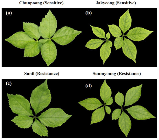
Figure 1.
Color image of ginseng plants in four varieties of sensitive (a,b) and resistant (c,d), respectively.
2.2. Fluorescence Hyperspectral Imaging System
Line-scan fluorescence hyperspectral imaging (Fl-HSI) in the VIS-NIR spectral range of 400 to 1000 nm was used for the non-destructive screening of ginseng plants. The main components of the HIS system, which is illustrated in (Figure 2), included a line-scan spectrograph (Headwall Photonics, Fitchburg, MA, USA), a c-mount objective lens (F/1.9 35 mm compact lens, Schneider Optics, Hauppauge, NY, USA), and an electron-multiplying charge-coupled device (EMCCD) camera (MegaLuca R, ANDOR Technology, South Windsor, CT, USA) with 1004 (spatial) × 1002 (spectral) pixels, which operates at a maximum pixel-readout rate of 12.5 MHz. The system was also equipped with a thermo-electric cooling system (−20 °C). The illumination system used two ultraviolet lamps (UV-365 nm, LED) (LZ4-40UA10, Ledengin Inc., Mansfield, OH, USA) as the excitation source for the materials. In general, fluorescence studies are employed in the spectrum radiation range between 400 nm to the far-red region at 750 nm. Since the system covers the range between 400–1000 nm, and the excitation and emission of the lights are between 400–750 nm, the light over the required range needed to be blocked to avoid an insensitive fluorescence spectrum in the data. Therefore, a bandpass filter was used to block light over 750 nm; a bandpass filter delivers a precisely defined range of spectral bands and blocks the signals out of the specified range.
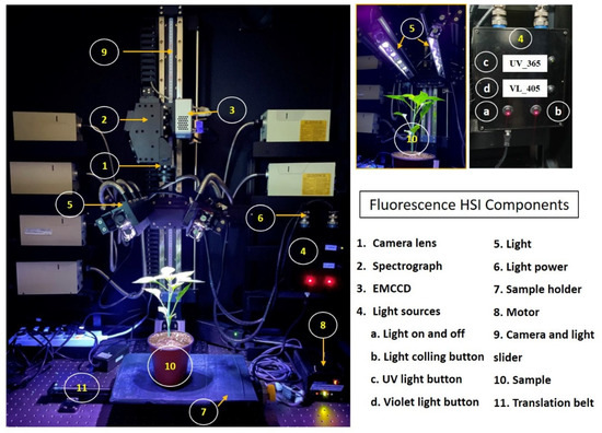
Figure 2.
Hyperspectral imaging system used for data collection.
2.3. Image Acquisition and Correction
A total of 80 ginseng plants, including four varieties with 20 plants each, were imaged before and after being subjected to heat-stress conditions using the Fl-HSI system in a dark room due to fluorescence sensitivity to ambient light [43,44] During the preliminary study, we imaged samples in a controlled environment. We validated heat-stressed ginseng plants’ excitation and emission wavelengths using a fixed-excitation lighting system of 365 nm ultraviolet (UV) light and an emission wavelength between 400 and 750 nm. Therefore, the samples were placed 40 cm from the lens on a conveyor. The samples were then scanned line-by-line in a dark chamber. Next, the images were saved in a three-dimensional (3D) “. Img” format consisting of spectral and spatial dimensions. The size of the raw hypercube was 502 pixels in the x-direction, n pixels in the y-direction (depending on the length of the plant samples), and 128 bands in the λ direction. Each image was corrected by subtracting the captured dark image (>0% reflectance); the dark image was obtained with the UV light turned-off, and the camera lens was entirely covered with its opaque cap. Other calibrated images were segmented from the background using the threshold reflectance value to remove non-uniform illumination from the imaged plants and visualize the reflectance value for further data extraction, as demonstrated in Figure 3.
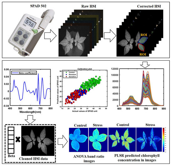
Figure 3.
Schematic representation showing data and analysis.
2.4. Data Extraction and Analysis
2.4.1. Spectral Extraction and Preprocessing
The corrected hyperspectral images extracted the 400–1000 nm spectral data from the region of interest (ROI) for each plant’s leaves. Since the bandpass filter blocks any light beyond 750 nm, we used a spectral range between 400–750 nm for further analysis. The mean spectrum of each plant’s ROI from all varieties before heat treatment in controlled plants, with 300 extracted spectral data points and 300 spectral data points, both from individual leaves, was obtained from plants after heat treatment in resistant and sensitive plants. Since the first two varieties were sensitive, and the last two were high temperature-resistant, we extracted spectral data from the susceptible varieties and combined them into a single group. The exact process combined the extracted spectra for two resistant varieties. For further analysis, a total of 600 spectral data points (from control, resistant, and sensitive plants) were obtained under both conditions for control and heat-stressed plants. The data were divided into 70% for calibration and 30% for validation. The spectral data were preprocessed to correct random noise caused by non-uniform illumination and light scattering generated by instruments, path length, and non-uniformity. Hence, it was essential to preprocess the extracted spectral data through appropriate mathematical algorithms to visualize the crucial information embedded in the plants and eliminate unwanted variation from the extracted data. Multiple studies have reported the preprocessing for data pretreatment [45,46,47,48,49]. In the present study, we applied normalization multiplicative scatter correction (MSC), smoothing, standard normal variate (SNV), and Savitzky–Golay first and second derivative approaches, which the detailed information related to each preprocessing reviewed [50]. Figure 4a,b illustrates the preprocessed spectral data plot and visualizes differences between plotted spectral data.
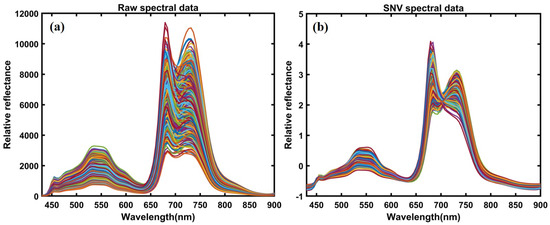
Figure 4.
(a) Raw spectral data; (b) SNV-based preprocessed spectral data.
2.4.2. Analysis of Variance and Waveband Selection
Hyperspectral imaging involves high dimensionality, broad adjacent wavelengths, and high-resolution spatial data, which increase the amount of information related to the measured number of samples. Selecting optimal wavelengths reduces the complexity of the image-processing pipeline and affords a better understanding of the different bands between our targets. For this purpose, ANOVA was employed to determine the significant wavebands to differentiate between control and stressed ginseng plants. However, because ANOVA is a statistical model that calculates variations between groups of data and provides useful descriptive information, it does not provide information related to the correlation of the groups within the entire computation. For this analysis, the extracted spectral data were divided into calibration (70%) and validation (30%). The control and stressed ginseng plants were calculated through the whole range from 400–750 nm to identify the optimal wavelength that was determined using the F-value of one-way ANOVA for discrimination.
2.4.3. Ratio Image for the Differentiation and Visualization of Heat-Stressed Plants
Initially, the obtained hyperspectral images were corrected as described in Section 2.3. Each imaged plant sample consisted of 128 bands ranging from 400 to 1000 nm. Then, the ANOVA-selected optimal wavelengths were divided (731.6 and 745.9 nm), as presented in Equation (1), for the band ratio image, generating a ratio image.
IR = IB1 (731 nm)/IB2 (745 nm)
Whereas the equation presents the IR (image ratio), IB1 (image band at 731 nm) divided by IB2 (image band two 745 nm) is suggested by ANOVA.
The thresholding value was determined by converting the ratio images to binary. The value was set based on the control and stressed plants’ average median pixel intensity. This process was based on using the median threshold intensity responses to visualize variations between heat-stressed and control ginseng plants (see Figure 5). In this process, the value intensity was determined to be less than or equal to the threshold computed for the control plants. Otherwise, the plant was classified as a stressed plant. The total performance of the thresholding method was evaluated based on calculating the sensitivity, specificity, and total accuracy using Equation (2), Equation (3), and Equation (4), respectively.
where in this study, true positive (TP) is a positive response for a positive condition that indicates the number of correctly detected stressed plants. A false positive (FP) is a positive response for a negative condition that indicates the number of control plants identified as stressed plants. A false negative (FN) is a negative response for a positive condition, implying the number of stressed plants detected as control plants. True negative (TN) is a negative response for a negative condition, referring to the number of correctly detected control plants.
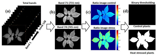
Figure 5.
Critical steps for generating band ratio images: (a) the cleaned background-free hyperspectral image, (b) an image of bands selected by ANOVA, (c) ratio image resulting from dividing 731.6/745.9 nm, (d) thresholding ratio image of the control presenting a black-and-white image of a stressed plant.
2.4.4. Reference Measurements SPAD-502
The SPAD-502 is a hand-held device commonly used to estimate nitrogen deficiency, and the greenness content directly influences chlorophyll concentration in leaves [51,52]. These correspondence SPAD readings depict the greenness of plants by transmitting light from light-emitting diodes at 650 nm and 940 nm, and the level of SPAD is defined as in Equation (5):
where the S(650) and S(940) are the signal without plant samples, S′(650) and S′(940) are the signal with samples, and B and C are constantly adjustable in the device software. The SPAD readings’ measurements are computed by an inherently built microprocessor based on the variation in the light attenuation. In general, the SPAD meter generates instantly non-destructive measurements ranging from 0 to 50 units. According to earlier research based on the wet chemistry determination of chlorophyll composition, the SPAD readings have a significant correlation to the quantity of chlorophyll composition in plants. However, the experimental measurements by SPAD do not indicate the chlorophyll concentration [53]. For example, the chlorophyll concentration of Arabidopsis thaliana plants was predicted with R2 = 0.9809 based on the SPAD unit [54,55,56].
2.4.5. Model Development
A partial least squares regression (PLSR) model was used to predict the greenness composition in the control and stressed ginseng plants. First, the greenness range in each leaf was quantified from 3 portions using a SPAD-502 plus chlorophyll meter (Konica Minolta, Inc., Osaka, Japan) and averaged as a corresponding reference value for the relevant leaf.
The PLSR algorithm is a widely used regression method for processing a large amount of data to predict the dependent variables by observing the relevant independent variables [57,58,59,60]. Furthermore, PLSR is used to explore the foundational correlations between x and y variables, and these findings enable the model to predict the composition of the y variables. The following equations demonstrate the PLSR model:
where x and y are the independent and dependent variables, T and U represent the score matrices, and indicate the x and y variable loading, and E represents the matrix error or residual.
The x-axis corresponds to the spectral data extracted from the ROI of the plants, and the Y-matrix contains the composition of each leaf measured by SPAD-502. The model was trained based on a calibration set of data and validation. Selecting the optimal number of latent variables (LV) helped avoid overfitting and underfitting in the model based on the minimum value of the root mean square error by applying Equation (8), based on the cross-validation. This technique is broadly applied in chemometrics and NIR data analysis [61,62].
where is the actual chlorophyll reference value of ginseng plants, is the value of the parameter predicted by the PLSR model, and z is the number of predictions.
Additionally, stepwise regression (SR) methods were applied to define influential bands for predicting SPAD readings from hyperspectral images. The SR is an effective method for selecting the variables depending on their capability to improve the performance of multilinear regression (MLR) models [63]. Stepwise regression statistically adds and removes variables from a model by reading their characteristics in regression. This method determined the p value of an F-statistic at each stage along this process-testing model with and without the optimal variable [64]. The stepwise selection methods consisted of forward and backward variable determination, which employed forward bands’ selection to avoid replicating variables with a thresholding maximum of 0.5 p-value.
3. Results
3.1. Spectral Profile of Ginseng Plants
Figure 6a presents the raw mean spectral data, and Figure 6b presents the SNV preprocessed spectral data extracted from the ROI of the leaves in the range of 400–900 nm. As can be seen, the only difference observed was in the magnitude of absorbance within the same group of spectral plants. Significant differences can be observed between the control and heat-stressed (resistant and sensitive) mean spectra of the ginseng plants in Figure 6a. These differences are more evident with sharper peaks after the preprocessing treatments presented in Figure 6b.
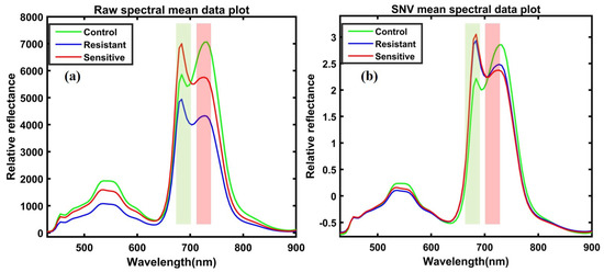
Figure 6.
(a) Total spectral data before preprocessing treatment and (b) spectral data after preprocessing.
3.2. SPAD Measurements Results
Higher SPAD readings represent more chlorophyll in plants; Figure 7 depicts the mean value of the total measured SPAD unit before and after heat treatment. However, the changes appeared in both group-resistant and sensitive ginseng plants; in comparison, resistant plants demonstrated different degrees of susceptibility.
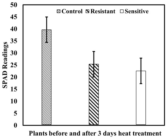
Figure 7.
Reference measurements of SPAD values.
3.3. ANOVA Analysis
Band Ratio Images for the Visualization of Stressed Plants
According to Figure 8, the highest F-values at 731 and 745 nm correspond to discrimination between the two groups of plants, with a threshold of 2.08 with 96.26% overall accuracy. The obtained results are based on the calibration data, which shows the critical wavelengths for discriminating stressed ginseng plants from the control. However, the range from 680 nm to 735 nm presented prominent bands with sharper peaks. The primary purpose of this approach was to determine the optimal thresholding value that corresponds to the detection of stressed plants based on the ratio image generated in response to the averaged intensity pixel value of the plants. Hence, the intensity pixel values for sensitive and resistant groups of samples in the stressed group were observed to be different. Therefore, it was essential to determine the optimal thresholding value in the responses of different bands combined with the range of observed changes based on conformation by the ANOVA results, which are plotted in Figure 8 and show the range between 600 and 830 nm for better visualization.
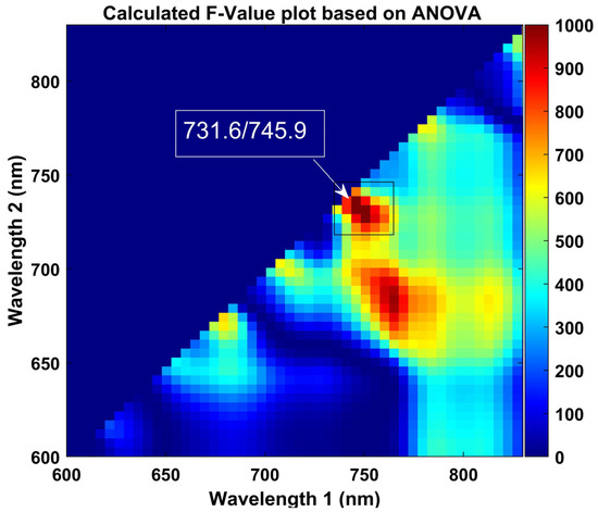
Figure 8.
Obtained F-value of two-band ratio (731.6/745.9) by one-way ANOVA. The color scale on the right side of the contour plot presents the increase in F-values from blue to red.
Additionally, we combined different range bands with the suggested bands from 683 to 745 nm and calculated each band’s combination performance based on correctly detecting the number of control and stressed plants (see Table 1). The higher F-value indicates more convenient discrimination relative to our targets. The computed maximum F-value is marked in Figure 8.

Table 1.
Statistical analysis of two optimal wavebands for discriminating between the control and stressed plants based on the ratio image to find the optimal thresholding value.
Consequently, Table 1 shows the generated ratio images based on (F683.9/F731.6) bands plotted in Figure 9a–d and Figure 9e–h, providing a clear discrimination of stressed ginseng plants, respectively, that presented a high accuracy of 98% using a 1.12 threshold value. However, the results closely correlate with the exact bands suggested by ANOVA, with 96.26% accuracy. As seen in Figure 9, the image ratio visualizations based on spatial information from the surfaces of the plants showed that the sensitive groups (a,b) of plants were slightly more affected than the resistant (c,d) groups of plants. After heat treatment, the images represent the affected range, from blue to red. Specifically, the sensitive plants are closer to yellow (e,f) than the resistant plant (g,h) group on the color bar east of the y-axis in Figure 9. Additionally, the changes can be observed based on the color bar on the right side of the plot on the y-axis.
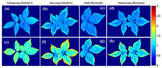
Figure 9.
Resulting images visualizing the control (top) and heat-stressed ginseng plants (bottom): (a,b) before being subjected to heat stress; (e,f) after exposure to heat stress. Images in (c,d) show plants before exposure to heat stress, and (g,h) are after heat treatments.
3.4. PLSR Model Performance
The prediction model was developed based on multiple preprocessing techniques, and the best-performing preprocessing model was used for further analysis, as shown in Table 2. Among the various preprocessing methods, the raw spectra-based model exhibited the best performance. As a result, the scatter plot in Figure 10a,b shows a strong correlation between the actual measured chlorophyll quantity in the plants and the predicted amount of chlorophyll in the meter readings.
Table 2.
PLSR results were obtained to predict the ginseng plants’ greenness composition.
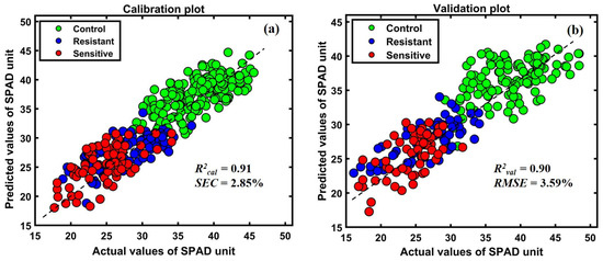
Figure 10.
(a) Calibration (b) validation plots of the established PLSR model.
As shown in Table 2, the raw preprocessing presented high accuracy among all preprocessing methods, with lower errors. The calibration correlation between the spectra and the chemical content of plants was high, with an R2calib value of 0.91. At the same time, the model validation had an R2val of 0.90 based on raw preprocessing, with a RMSEV of 3.59%. Based on the comparison in Table 2, the determination coefficient of calibration and prediction was over 0.91 for all developed models. The plots in Figure 10a,b show the calibration and prediction results, respectively. The y-axis corresponds to the measured plant’s greenness composition value based on SPAD-502, and the x-axis represents the predicted SPAD-measured composition as a linear correlation of calibration and prediction.
According to the plotted results in Figure 10, the red color indicates lower holding SPAD values compared to the resistant plants. The calibration and validation data plot distributions follow the consistency of Figure 6a,b spectral means and generated ratio images in Figure 9.
Furthermore, this study used the beta coefficient of the PLSR model to estimate the chemical distribution of greenness contents in both the control and stressed ginseng plants. Figure 11 shows the beta coefficient, where the peaks at around 680 nm to 745 nm represent chlorophyll spectral peaks. Different analyses reported the composition corresponding to exact bands or closely around the most visible bands, and most vitally in related peaks observed in our study, circled in Figure 11.
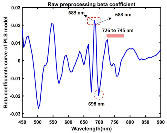
Figure 11.
Beta coefficient curve from the partial least squares regression model for predicting leaves’ green-level contents in ginseng plants.
The chemical mapping of the ginseng plants presented in Figure 12 and Figure 13 shows the spatial distribution of the greenness level on the surfaces of leaves and has a high correlation to chlorophyll concentration, which is essential for determining pigment composition in plants. Therefore, the potential concentration of greenness in plants was determined via chemical mapping, in which the color scale from blue to red in the y-axis of Figure 12 and Figure 13 represents the chemical concentration, or the plants with more greenness, consisting of more chlorophyll concentration. Additionally, the intensity representation of each group of plants was plotted on a histogram to better visualize changes in the plants. In the histogram plots, the x-axis indicates the responses to the intensity of pixels, and the y-axis corresponds to the number of pixels at each intensity value presented by the image.
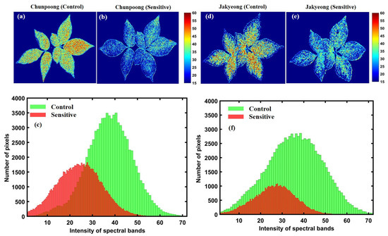
Figure 12.
The first variety before (a) and after (b) subjecting to heat stress; (c) represents a related histogram. The second variety before (d) and after (e) heat exposure; (f) represents a related histogram.
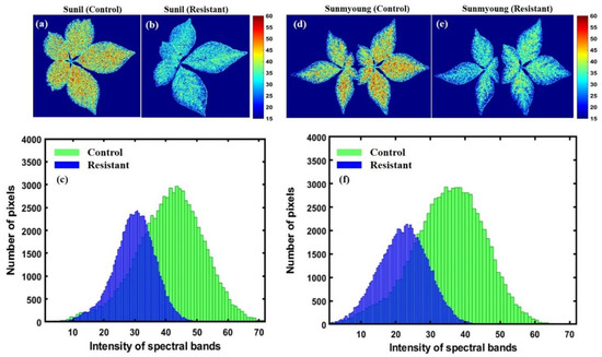
Figure 13.
First variety before (a) and after (b) subjecting to heat stress; (c) represents a related histogram. Second resistant variety before (d) and after (e) heat exposure; (f) represents a related histogram of predicted PLS images.
Accordingly, Figure 12a–c presents the chemical properties of Chunpoong variety-related plants after exposure to heat stress, which shows significant greenness level changes with similar patterns in the second sensitive variety (Jakyeong), with a clear representation of the chemical images and plotted histogram in Figure 12d–f, respectively.
In the same manner, Figure 13 demonstrates the same SPAD measurement level scenario as susceptible varieties. However, the plants’ sensitivity and resistance in both groups were affected by high temperatures.
Furthermore, the stepwise regression (SR) band selection approach was observed at 683 nm, 688 nm, 703 nm, 731 nm, and 745 nm from the full bands; these suggested five bands are included, and two optimal bands were selected by ANOVA to develop a PLSR model that performed with a R2val of 0.81 and a RMSEV of 4.74%. The determined beta coefficient based on the five-band model was applied to each, concerning the same bands, to visualize the chemical composition of imaged plants. Figure 14 shows the mapping of greenness levels before and after subjecting to heat stress. The color bar in the x-axis of Figure 14, ranging the SPAD values from 15–60, shows the distribution of the greenness quantity in plants: from blue to darker red, the chlorophyll content increases.
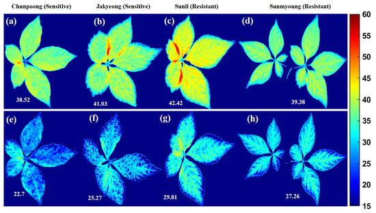
Figure 14.
Plants (a–d) before heat stress and (e–h) after subjecting to heat stress, concerning each variety.
4. Discussion
4.1. Spectral Analysis
In the current investigation, emissions occurred between 450 and 600 nm and 625 and 750 nm. However, as demonstrated in the SNV-based preprocessed spectral data in Figure 6b, reflectance increased substantially, with wavelengths from around 680 to 731 nm, with sharper peaks due to internal light scattering by the leaf cells. At the same time, the reflectance in the visible range was lower due to light absorption by leaf pigments in the visible region between 450 and 636 nm. There are significant intensity variations across the spectral curve of the samples, with control plants having higher reflectance in the near-infrared region than stressed plants. Since healthy plants reflect more light than unhealthy plants in the near-infrared region over 700 nm, heat-stressed plants that presented a higher intensity in the visible range might have less greenness and chlorophyll composition, which reflects more light from the surface of the leaves. However, in the visible region, there were some overlaps between control and stressed ginseng spectral mapping due to a higher moisture content in healthy plants.
In comparison, the sensitive group was vulnerable to heat treatment, because the peaks represent changes in order, with Figure 6b mapping order changes in the peaks at 683 nm in the visible region. Apart from peaks at the near-infrared region of 731 nm, higher peaks correspond to control, resistance, and sensitive plants. Various studies have reported peaks at around 680 and 735 nm corresponding to plants’ chlorophyll absorption. For instance, early-stage disease detection in grapefruit plants appeared at around 686 nm and 735 nm [39], and early blight and late blight disease in tomato leaves’ chlorophyll bands were detected at 680 nm [65]. In another study, drought-stressed soybean plants presented chlorophyll (a) peaks at around 686 and 738 nm [30], and for assessment yield in cowpea plants, chlorophyll peaks were observed at the same peaks, at around 683 nm and 731 nm [66]. Overall, we concluded that peaks at 683 nm and 731 nm corresponded with chlorophyll peaks in control and heat-stressed ginseng plant leaves.
4.2. Reference Measurement Analysis
Since the SPAD measurements are applicable for small areas and are less efficient for frequently monitoring a large field area, in this work, unlike the chlorophyll meter, the spectral features of the plants ranged between 400–1000 nm, consisting of 128 bands extracted from the ROI of each leaf. These obtained mean spectra correlated with measured SPAD readings of those leaves for further model development and analysis. The chlorophyll meter readings in the plants are shown in Figure 7, in which the resistant and sensitive varieties showed slightly different changes due to heat stress impacting both varieties, which might be a close range of greenness levels. Additionally, the chlorophyll meter readings can be impacted by several factors, including the environment and crop leaf properties. Further, anything else that may affect plant color (e.g., diseases, nutritional deficits, variety variances) can affect chlorophyll meter results [67,68]. Furthermore, among the environmental factors, heat stress severely impacts the plants’ declining chemical properties, specifically the chlorophyll composition, as reported previously [69,70]. Therefore, the declining mean value of measured relative chlorophyll compositions potentially demonstrated the consequences of heat-stress on the ginseng plants.
4.3. ANOVA Results Analysis
The bands suggested by ANOVA demonstrated a vital role in identifying heat-stressed plans, and the optimally selected bands with the high-performance binary classification of plants were based on the suggested bands at 731 nm and 745 nm, as shown in Table 1. However, the ANOVA provides descriptive bands for discrimination between the classes, which showed that bands classified the classes with a 96% accuracy. A reduction in plants’ greenness due to heat stress caused a decline in chlorophyll composition, and the chlorophyll bands in the control and stressed plants offered a classification of 98% accuracy based on generated ratio images.
4.4. PLSR Results Analysis
Among different preprocessing approaches, raw preprocessing demonstrated a higher accuracy, as plotted in Figure 10, with compatibility in the observed changes, respectively, in the mean spectral data in Figure 6 and the demonstrated mean SPAD values in Figure 7. Furthermore, the obtained beta coefficient was used to develop a chemical visualization of the control and stressed plants. The observed peaks in the beta coefficient at 683 nm and 731 nm, previously discussed in the spectral interpretation of data, correlated to chlorophyll bands. According to previous reports, the peaks at around 683 nm [71] and 688 nm are related to reflectance bands of chlorophyll emission [36,67]. Furthermore, the peaks at around 683 nm and 731 nm [66], peaks around 698 nm [72], are reported as the chlorophyll bands, and there are other bands around the region of 726 nm and 745 nm corresponding to chlorophyll emissions [30,47]. Thus, this study demonstrates the potential of hyperspectral fluorescence imaging for predicting plant-relative chlorophyll compositions in plant leaves.
Hyperspectral imaging has significant potential for the early visualization of chemical composition changes in abiotically stressed plants, including disease detection in tobacco plants [18]. For example, other research has reported the image-based visualization of changes in chemical properties, detection of the severity as well as the quantification of Pseudomonas Cichorii in tomato plants (using hyperspectral fluorescence imaging) [31], the determination of nitrogen distribution in pepper plants [73], the detection of freezing stress in wheat plants [74], and prediction of nicotine content in tobacco [75].
For this purpose, the corrected hyperspectral image was processed to visualize the correlation between greenness and chemical composition changes in ginseng plants. In contrast, the resistant groups of plants were less susceptible or more resistant than the sensitive groups of plants. Furthermore, the chemical images showed that the sensitive groups of plants were more vulnerable to high temperatures than the resistant group (see Figure 13a–f). Additionally, the same pattern was observed in the histogram representations, in which the stressed plants from resistant varieties showed the most significant number of pixels corresponding to the highest intensity peaks (over 2500 pixels; see Figure 13c,f). At the same time, the most significant number of pixels in the stressed plants corresponded to sensitive groups (1000 to 1700 pixels; see Figure 12c,f). In this way, the present study confirmed the resistance of Suni and Sunmyoung for two sensitive groups, Chunpoong and Jakyeong. However, this study did not correlate the chlorophyll concentrations with spectral features. Instead, the SPAD readings presented a mapping of greenness levels in plants, with the general theory that plants with higher greenness levels will consist of higher chlorophyll concentrations.
Despite significant advantages, the hyperspectral fluorescence measurements require the adaptation of the plants to the dark and limit their application for outdoor phenotyping. Despite breakthroughs in fluorescence imaging technologies, SIF transcends the dark adaptation phase and can be used as an alternative. These approaches may be applicable in different scales and present considerable potential, though they do not visualize the absolute photosynthetic biochemistry of plant data. However, these approaches still require considerable modification [76]. Therefore, more research and novel non-destructive real-time operating systems are required to evaluate plant status. Furthermore, farmers and investors are more interested in low-cost devices for detecting unhealthy crops. In our future work, we will consider developing low-cost imaging with the influential bands observed in this study based on the ANOVA, at 683 nm and 731 nm, for discrimination, as well as the observed bands based on SR, at 683 nm, 688 nm, 703 nm, 731 nm, and 745 nm, for the prediction of relative chlorophyll composition in ginseng plants, as demonstrated in Figure 14.
Recently, low-cost components and optical parts have improved fluorescence imaging applications for field- and laboratory-based phenotyping. For example, multicolor fluorescence imaging was developed for salt stress detection in Arabidopsis. A second study reported a low-cost fluorescence system for stress detection in plants, and detailed information on the systems’ setups can be found in the reported studies [60,77]. As an alternative to SPAD meters, a low-cost imaging system might be more affordable and convenient for measuring the chlorophyll or greenness level of plants. However, the embedded imaging system might be slightly larger than those devices that are currently employed due to the inclusion of imaging sensors, illumination units, microprocessors, and screens for real-time display capacity. Instead, farmers can employ a well-built and thoroughly tested imaging system for fast, non-destructive, and portable real-time applications for potentially monitoring large fields in less time.
5. Conclusions
In the present study, hyperspectral fluorescence imaging in the spectral range of 400–1000 nm was used to detect and predict relative chlorophyll composition in sensitive and heat-resistant ginseng plants. ANOVA-determined wavelengths of 683 nm and 731 nm were used for the generation of a ratio image that was completed with 98% discrimination accuracy. Furthermore, individual quantitative PLSR models with appropriate preprocessing approaches were established based on the full-band spectral data, yielding good results with a coefficient of R2val = 0.90 and a RMSEV = 3.59%. Additionally, using stepwise regression (SR) analysis on the observed bands resulted in a R2val of 0.81 and a RMSEV of 4.74%. By applying the obtained beta coefficient in the PLSR regression model, chemical visualization maps were generated to predict the level of chlorophyll composition relative to each pixel in the images. This chemical map created with a pixel-wise approach helped to evaluate the greenness level or relative chlorophyll concentration patterns of the control, sensitive, and resistant plants. The sensitive ginseng plants were affected more strongly than the resistant varieties, and the same pattern was observed in the PLS image of each variety. These findings indicate that the observed influential bands by ANOVA and SR could be applicable for developing low-cost and portable instruments for the early-stage evaluation of ginseng plants.
Author Contributions
Conceptualization, B.-K.C. and E.P.; methodology, M.A.F.; software, M.S.K. and I.B.; validation, E.P., M.A.F. and R.J.; formal analysis, M.A.F. and J.K.; investigation, E.P.; resources, B.-K.C., T.K. and M.A.F.; data curation, E.P.; writing—original draft preparation, M.A.F.; writing—review and editing, B.-K.C.; visualization, M.A.F. and E.P.; supervision, B.-K.C.; project administration, B.-K.C.; funding acquisition, B.-K.C. All authors have read and agreed to the published version of the manuscript.
Funding
This research was supported by the Korea Institute of Planning and Evaluation for Technology in Food, Agriculture, and Forestry (IPET) through the Smart Farm Innovation Technology Development Program, funded by the Ministry of Agriculture, Food, and Rural Affairs (MAFRA) (421030-04).
Institutional Review Board Statement
Not applicable.
Informed Consent Statement
Not applicable.
Data Availability Statement
Not applicable.
Conflicts of Interest
The authors declare no conflict of interest.
References
- Park, J.E.; Kim, H.; Kim, J.; Choi, S.J.; Ham, J.; Nho, C.W.; Yoo, G. A Comparative Study of Ginseng Berry Production in a Vertical Farm and an Open Field. Ind. Crops Prod. 2019, 140, 111612. [Google Scholar] [CrossRef]
- Park, H.J.; Kim, D.H.; Park, S.J.; Kim, J.M.; Ryu, J.H. Ginseng in Traditional Herbal Prescriptions. J. Ginseng Res. 2012, 36, 225–241. [Google Scholar] [CrossRef] [PubMed]
- Karmalkar, A.V.; Bradley, R.S. Consequences of Global Warming of 1.5 °c and 2 °c for Regional Temperature and Precipitation Changes in the Contiguous United States. PLoS ONE 2017, 12, 1–17. [Google Scholar] [CrossRef] [PubMed]
- Mo, H.S.; Jang, I.B.; Yu, J.; Park, H.W.; Park, K.C. Effects of Enhanced Light Transmission Rate During the Early Growth Stage on Plant Growth, Photosynthetic Ability and Disease Incidence of Above Ground in Panax Ginseng. Korean J. Med. Crop Sci. 2015, 23, 284–291. [Google Scholar] [CrossRef]
- Kim, S.W.; Gupta, R.; Min, C.W.; Lee, S.H.; Cheon, Y.E.; Meng, Q.F.; Jang, J.W.; Hong, C.E.; Lee, J.Y.; Jo, I.H.; et al. Label-Free Quantitative Proteomic Analysis of Panax Ginseng Leaves upon Exposure to Heat Stress. J. Ginseng Res. 2019, 43, 143–153. [Google Scholar] [CrossRef]
- Hong, J.; Geem, K.R.; Kim, J.; Jo, I.H.; Yang, T.J.; Shim, D.; Ryu, H. Prolonged Exposure to High Temperature Inhibits Shoot Primary and Root Secondary Growth in Panax Ginseng. Int. J. Mol. Sci. 2022, 23, 11647. [Google Scholar] [CrossRef]
- Hwang, C.R.; Lee, S.H.; Jang, G.Y.; Hwang, I.G.; Kim, H.Y.; Woo, K.S.; Lee, J.; Jeong, H.S. Changes in Ginsenoside Compositions and Antioxidant Activities of Hydroponic-Cultured Ginseng Roots and Leaves with Heating Temperature. J. Ginseng Res. 2014, 38, 180–186. [Google Scholar] [CrossRef]
- Lee, J.S.; Lee, K.H.; Lee, S.S.; Kim, E.S.; Ahn, I.O.; In, J.G. Morphological Characteristics of Ginseng Leaves in High-Temperature Injury Resistant and Susceptible Lines of Panax Ginseng Meyer. J. Ginseng Res. 2011, 35, 449–456. [Google Scholar] [CrossRef]
- Jayakodi, M.; Lee, S.C.; Yang, T.J. Comparative Transcriptome Analysis of Heat Stress Responsiveness between Two Contrasting Ginseng Cultivars. J. Ginseng Res. 2019, 43, 572–579. [Google Scholar] [CrossRef]
- Mittler, R. Abiotic Stress, the Field Environment and Stress Combination. Trends Plant Sci. 2006, 11, 15–19. [Google Scholar] [CrossRef]
- Persons, S.W.; Davis, J. Growing Ginseng Under Artificial Shade. Available online: https://www.wildgrown.com/index.php/growing-ginseng/120-growing-ginseng-under-artificial-shade (accessed on 10 November 2022).
- Jia, L.; Zhao, Y. Current Evaluation of the Millennium Phytomedicine- Ginseng (I): Etymology, Pharmacognosy, Phytochemistry, Market and Regulations. Curr. Med. Chem. 2009, 16, 2475–2484. [Google Scholar] [CrossRef] [PubMed]
- Kim, Y.J.; Nguyen, T.K.L.; Oh, M.M. Growth and Ginsenosides Content of Ginseng Sprouts According to Led-Based Light Quality Changes. Agronomy 2020, 10, 1979. [Google Scholar] [CrossRef]
- Kim, Y.J.; Zhang, D.; Yang, D.C. Biosynthesis and Biotechnological Production of Ginsenosides. Biotechnol. Adv. 2015, 33, 717–735. [Google Scholar] [CrossRef] [PubMed]
- Kolhar, S.; Jagtap, J. Plant Trait Estimation and Classification Studies in Plant Phenotyping Using Machine Vision – A Review. Inf. Process. Agric. 2021. [Google Scholar] [CrossRef]
- Cotrozzi, L.; Couture, J.J. Hyperspectral Assessment of Plant Responses to Multi-Stress Environments: Prospects for Managing Protected Agrosystems. Plants People Planet 2020, 2, 244–258. [Google Scholar] [CrossRef]
- Fahrentrapp, J.; Ria, F.; Geilhausen, M.; Panassiti, B. Detection of Gray Mold Leaf Infections Prior to Visual Symptom Appearance Using a Five-Band Multispectral Sensor. Front. Plant Sci. 2019, 10, 1–14. [Google Scholar] [CrossRef]
- Gu, Q.; Sheng, L.; Zhang, T.; Lu, Y.; Zhang, Z.; Zheng, K.; Hu, H.; Zhou, H. Early Detection of Tomato Spotted Wilt Virus Infection in Tobacco Using the Hyperspectral Imaging Technique and Machine Learning Algorithms. Comput. Electron. Agric. 2019, 167, 105066. [Google Scholar] [CrossRef]
- Asaari, M.S.M.; Mertens, S.; Dhondt, S.; Inzé, D.; Wuyts, N.; Scheunders, P. Analysis of Hyperspectral Images for Detection of Drought Stress and Recovery in Maize Plants in a High-Throughput Phenotyping Platform. Comput. Electron. Agric. 2019, 162, 749–758. [Google Scholar] [CrossRef]
- Sánchez, M.T.; Entrenas, J.A.; Torres, I.; Vega, M.; Pérez-Marín, D. Monitoring Texture and Other Quality Parameters in Spinach Plants Using NIR Spectroscopy. Comput. Electron. Agric. 2018, 155, 446–452. [Google Scholar] [CrossRef]
- Kasampalis, D.S.; Tsouvaltzis, P.; Ntouros, K.; Gertsis, A.; Gitas, I.; Siomos, A.S. The Use of Digital Imaging, Chlorophyll Fluorescence and Vis/NIR Spectroscopy in Assessing the Ripening Stage and Freshness Status of Bell Pepper Fruit. Comput. Electron. Agric. 2021, 187, 106265. [Google Scholar] [CrossRef]
- Swarup, A.; Lee, W.S.; Peres, N.; Fraisse, C. Strawberry Plant Wetness Detection Using Color and Thermal Imaging. J. Biosyst. Eng. 2020, 45, 409–421. [Google Scholar] [CrossRef]
- Raza, S.E.A.; Prince, G.; Clarkson, J.P.; Rajpoot, N.M. Automatic Detection of Diseased Tomato Plants Using Thermal and Stereo Visible Light Images. PLoS ONE 2015, 10, e0123262. [Google Scholar] [CrossRef] [PubMed]
- Zhuang, S.; Wang, P.; Jiang, B.; Li, M.; Gong, Z. Early Detection of Water Stress in Maize Based on Digital Images. Comput. Electron. Agric. 2017, 140, 461–468. [Google Scholar] [CrossRef]
- Zhou, S.; Mou, H.; Zhou, J.; Zhou, J.; Ye, H.; Nguyen, H.T. Development of an Automated Plant Phenotyping System for Evaluation of Salt Tolerance in Soybean. Comput. Electron. Agric. 2021, 182, 106001. [Google Scholar] [CrossRef]
- Putra, B.T.W.; Amirudin, R.; Marhaenanto, B. The Evaluation of Deep Learning Using Convolutional Neural Network (CNN) Approach for Identifying Arabica and Robusta Coffee Plants. J. Biosyst. Eng. 2022, 47, 118–129. [Google Scholar] [CrossRef]
- Mishra, P.; Feller, T.; Schmuck, M.; Nicol, A.; Nordon, A. Early Detection of Drought Stress in Arabidopsis Thaliana Utilsing a Portable Hyperspectral Imaging Setup. In Proceedings of the 2019 10th Workshop on Hyperspectral Imaging and Signal Processing: Evolution in Remote Sensing (WHISPERS), Amsterdam, The Netherlands, 24–26 September 2019; pp. 1–5. [Google Scholar] [CrossRef]
- Mishra, P.; Feller, T.; Schmuck, M.; Nicol, A.; Nordon, A. Early Detection of Drought Stress in Arabidopsis Thaliana Utilsing a Portable Hyperspectral Imaging Setup WestCHEM; Department of Pure and Applied Chemistry and Centre for Process Analytics and Control Technology, University of Strathclyde: Glasgow, UK, 2019; pp. 2–6. [Google Scholar]
- Wang, D.; Vinson, R.; Holmes, M.; Seibel, G.; Bechar, A.; Nof, S.; Tao, Y. Early Detection of Tomato Spotted Wilt Virus by Hyperspectral Imaging and Outlier Removal Auxiliary Classifier Generative Adversarial Nets (OR-AC-GAN). Sci. Rep. 2019, 9, 4377. [Google Scholar] [CrossRef]
- Mo, C.; Kim, M.S.; Kim, G.; Cheong, E.J.; Yang, J.; Lim, J. Detecting Drought Stress in Soybean Plants Using Hyperspectral Fluorescence Imaging. J. Biosyst. Eng. 2015, 40, 335–344. [Google Scholar] [CrossRef]
- Rajendran, D.K.; Park, E.; Nagendran, R.; Hung, N.B.; Cho, B.K.; Kim, K.H.; Lee, Y.H. Visual Analysis for Detection and Quantification of Pseudomonas Cichorii Disease Severity in Tomato Plants. Plant Pathol. J. 2016, 32, 300–310. [Google Scholar] [CrossRef]
- Bauriegel, E.; Herppich, W.B. Hyperspectral and Chlorophyll Fluorescence Imaging for Early Detection of Plant Diseases, with Special Reference to Fusarium Spec. Infections on Wheat. Agriculture 2014, 4, 32–57. [Google Scholar] [CrossRef]
- Montero, R.; Pérez-Bueno, M.L.; Barón, M.; Florez-Sarasa, I.; Tohge, T.; Fernie, A.R.; El aou ouad, H.; Flexas, J.; Bota, J. Alterations in Primary and Secondary Metabolism in Vitis Vinifera ‘Malvasía de Banyalbufar’ upon Infection with Grapevine Leafroll-Associated Virus 3. Physiol. Plant. 2016, 157, 442–452. [Google Scholar] [CrossRef]
- Mazur, R.; Sadowska, M.; Kowalewska, Ł.; Abratowska, A.; Kalaji, H.M.; Mostowska, A.; Garstka, M.; Krasnodebska-Ostrega, B. Overlapping Toxic Effect of Long Term Thallium Exposure on White Mustard (Sinapis Alba L.) Photosynthetic Activity. BMC Plant Biol. 2016, 16, 89–101. [Google Scholar] [CrossRef] [PubMed]
- Wang, N.; Clevers, J.G.P.W.; Wieneke, S.; Bartholomeus, H.; Kooistra, L. Potential of UAV-Based Sun-Induced Chlorophyll Fluorescence to Detect Water Stress in Sugar Beet. Agric. For. Meteorol. 2022, 323, 109033. [Google Scholar] [CrossRef]
- Zarco-Tejada, P.J.; Pushnik, J.C.; Dobrowski, S.; Ustin, S.L. Steady-State Chlorophyll a Fluorescence Detection from Canopy Derivative Reflectance and Double-Peak Red-Edge Effects. Remote Sens. Environ. 2003, 84, 283–294. [Google Scholar] [CrossRef]
- Hernández-Clemente, R.; North, P.R.J.; Hornero, A.; Zarco-Tejada, P.J. Assessing the Effects of Forest Health on Sun-Induced Chlorophyll Fluorescence Using the FluorFLIGHT 3-D Radiative Transfer Model to Account for Forest Structure. Remote Sens. Environ. 2017, 193, 165–179. [Google Scholar] [CrossRef]
- Dong, X.; Kim, W.Y.; Lee, K.H. Drone-Based Three-Dimensional Photogrammetry and Concave Hull by Slices Algorithm for Apple Tree Volume Mapping. J. Biosyst. Eng. 2021, 46, 474–484. [Google Scholar] [CrossRef]
- Saleem, M.; Atta, B.M.; Ali, Z.; Bilal, M. Laser-Induced Fluorescence Spectroscopy for Early Disease Detection in Grapefruit Plants. Photochem. Photobiol. Sci. 2020, 19, 713–721. [Google Scholar] [CrossRef]
- Mahlein, A.-K. Present and Future Trends in Plant Disease Detection. Plant Dis. 2016, 100, 89–101. [Google Scholar] [CrossRef]
- Bodria, L.; Fiala, M.; Oberti, R.; Naldi, E. Chlorophyll Fluorescence Sensing for Early Detection of Crop’s Diseases Symptoms. In Proceedings of the 2002 ASAE Annual International Meeting, Chicago, IL, USA, 28–31 July 2002; pp. 1–15. [Google Scholar]
- Kuckenberg, J.; Tartachnyk, I.; Noga, G. Temporal and Spatial Changes of Chlorophyll Fluorescence as a Basis for Early and Precise Detection of Leaf Rust and Powdery Mildew Infections in Wheat Leaves. Precis. Agric. 2009, 10, 34–44. [Google Scholar] [CrossRef]
- Treibitz, T.; Neal, B.P.; Kline, D.I.; Beijbom, O.; Roberts, P.L.D.; Mitchell, B.G.; Kriegman, D. Wide Field-of-View Fluorescence Imaging of Coral Reefs. Sci. Rep. 2015, 5, 7694. [Google Scholar] [CrossRef]
- Norikane, J.H.; Kurata, K. Water Stress Detection By Monitoring Fluorescence of Plants under Ambient Light. Trans. ASAE 2001, 44, 1915–1922. [Google Scholar] [CrossRef]
- Faqeerzada, M.A.; Lohumi, S.; Kim, G.; Joshi, R.; Lee, H.; Kim, M.S.; Cho, B.K. Hyperspectral Shortwave Infrared Image Analysis for Detection of Adulterants in Almond Powder with One-Class Classification Method. Sensors 2020, 20, 5855. [Google Scholar] [CrossRef] [PubMed]
- Rahman, A.; Faqeerzada, M.A.; Cho, B.K. Hyperspectral Imaging for Predicting the Allicin and Soluble Solid Content of Garlic with Variable Selection Algorithms and Chemometric Models. J. Sci. Food Agric. 2018, 98, 4715–4725. [Google Scholar] [CrossRef] [PubMed]
- Park, E.; Kim, Y.S.; Omari, M.K.; Suh, H.K.; Faqeerzada, M.A.; Kim, M.S.; Baek, I.; Cho, B.K. High-Throughput Phenotyping Approach for the Evaluation of Heat Stress in Korean Ginseng (Panax Ginseng Meyer) Using a Hyperspectral Reflectance Image. Sensors 2021, 21, 5634. [Google Scholar] [CrossRef] [PubMed]
- Faqeerzada, M.A.; Perez, M.; Lohumi, S.; Lee, H.; Kim, G.; Wakholi, C.; Joshi, R.; Cho, B.K. Online Application of a Hyperspectral Imaging System for the Sorting of Adulterated Almonds. Appl. Sci. 2020, 10, 6569. [Google Scholar] [CrossRef]
- Rahman, A.; Faqeerzada, M.A.; Joshi, R.; Lohumi, S.; Kandpal, L.M.; Lee, H.; Mo, C.; Kim, M.S.; Cho, B.K. Quality Analysis of Stored Bell Peppers Using Near-Infrared Hyperspectral Imaging. Trans. ASABE 2018, 61, 1199–1207. [Google Scholar] [CrossRef]
- Rinnan, Å.; van den Berg, F.; Engelsen, S.B. Review of the Most Common Pre-Processing Techniques for near-Infrared Spectra. TrAC—Trends Anal. Chem. 2009, 28, 1201–1222. [Google Scholar] [CrossRef]
- Yuan, Z.; Cao, Q.; Zhang, K.; Ata-Ul-Karim, S.T.; Tan, Y.; Zhu, Y.; Cao, W.; Liu, X. Optimal Leaf Positions for SPAD Meter Measurement in Rice. Front. Plant Sci. 2016, 7, 1–10. [Google Scholar] [CrossRef]
- Uddling, J.; Gelang-Alfredsson, J.; Piikki, K.; Pleijel, H. Evaluating the Relationship between Leaf Chlorophyll Concentration and SPAD-502 Chlorophyll Meter Readings. Photosynth. Res. 2007, 91, 37–46. [Google Scholar] [CrossRef]
- Borhan, M.S.; Panigrahi, S.; Satter, M.A.; Gu, H. Evaluation of Computer Imaging Technique for Predicting the SPAD Readings in Potato Leaves. Inf. Process. Agric. 2017, 4, 275–282. [Google Scholar] [CrossRef]
- Ling, Q.; Huang, W.; Jarvis, P. Use of a SPAD-502 Meter to Measure Leaf Chlorophyll Concentration in Arabidopsis Thaliana. Photosynth. Res. 2011, 107, 209–214. [Google Scholar] [CrossRef]
- Xiong, D.; Chen, J.; Yu, T.; Gao, W.; Ling, X.; Li, Y.; Peng, S.; Huang, J. SPAD-Based Leaf Nitrogen Estimation Is Impacted by Environmental Factors and Crop Leaf Characteristics. Sci. Rep. 2015, 5, 13389. [Google Scholar] [CrossRef] [PubMed]
- Markwell, J.; Osterman, J.C.; Mitchell, J.L. Calibration of the Minolta SPAD-502 Leaf Chlorophyll Meter. Photosynth. Res. 1995, 46, 467–472. [Google Scholar] [CrossRef] [PubMed]
- Rahman, A.; Kandpal, L.M.; Lohumi, S.; Kim, M.S.; Lee, H.; Mo, C.; Cho, B.K. Nondestructive Estimation of Moisture Content, PH and Soluble Solid Contents in Intact Tomatoes Using Hyperspectral Imaging. Appl. Sci. 2017, 7, 109. [Google Scholar] [CrossRef]
- Lohumi, S.; Lee, S.; Cho, B.K. Optimal Variable Selection for Fourier Transform Infrared Spectroscopic Analysis of Starch-Adulterated Garlic Powder. Sensors Actuators B Chem. 2015, 216, 622–628. [Google Scholar] [CrossRef]
- Faqeerzada, M.; Rahman, A.; Kim, G.; Park, E.; Joshi, R.; Lohumi, S.; Cho, B.-K. Prediction of Moisture Contents in Green Peppers Using Hyperspectral Imaging Based on a Polarized Lighting System. Korean J. Agric. Sci. 2020, 47, 995–1010. [Google Scholar]
- Tian, Y.; Xie, L.; Wu, M.; Yang, B.; Ishimwe, C.; Ye, D.; Weng, H. Multicolor Fluorescence Imaging for the Early Detection of Salt Stress in Arabidopsis. Agronomy 2021, 11, 2577. [Google Scholar] [CrossRef]
- Tan, C.; Wang, J.; Wu, T.; Qin, X.; Li, M. Determination of Nicotine in Tobacco Samples by Near-Infrared Spectroscopy and Boosting Partial Least Squares. Vib. Spectrosc. 2010, 54, 35–41. [Google Scholar] [CrossRef]
- Tunny, S.S.; Amanah, H.Z.; Faqeerzada, M.A.; Wakholi, C.; Kim, M.S.; Baek, I.; Cho, B.K. Multispectral Wavebands Selection for the Detection of Potential Foreign Materials in Fresh-Cut Vegetables. Sensors 2022, 22, 1775. [Google Scholar] [CrossRef]
- Jin, J.; Wang, Q. Evaluation of Informative Bands Used in Different PLS Regressions for Estimating Leaf Biochemical Contents from Hyperspectral Reflectance. Remote Sens. 2019, 11, 197. [Google Scholar] [CrossRef]
- Draper, N.R.; Smith, H. Applied Regression Analysis; John Wiley & Sons: Hoboken, NJ, USA, 1998; pp. 1–716. [Google Scholar]
- Xie, C.; Shao, Y.; Li, X.; He, Y. Detection of Early Blight and Late Blight Diseases on Tomato Leaves Using Hyperspectral Imaging. Sci. Rep. 2015, 5, 16564. [Google Scholar] [CrossRef]
- Anderson, B.; Buah-Bassuah, P.K.; Tetteh, J.P. Using Violet Laser-Induced Chlorophyll Fluorescence Emission Spectra for Crop Yield Assessment of Cowpea (Vigna Unguiculata (L) Walp) Varieties. Meas. Sci. Technol. 2004, 15, 1255–1265. [Google Scholar] [CrossRef]
- Limantara, L.; Dettling, M.; Indrawati, R.; Indriatmoko; Brotosudarmo, T.H.P. Analysis on the Chlorophyll Content of Commercial Green Leafy Vegetables. Procedia Chem. 2015, 14, 225–231. [Google Scholar] [CrossRef]
- Nauš, J.; Prokopová, J.; Řebíček, J.; Špundová, M. SPAD Chlorophyll Meter Reading Can Be Pronouncedly Affected by Chloroplast Movement. Photosynth. Res. 2010, 105, 265–271. [Google Scholar] [CrossRef] [PubMed]
- Wassie, M.; Zhang, W.; Zhang, Q.; Ji, K.; Chen, L. Effect of Heat Stress on Growth and Physiological Traits of Alfalfa (Medicago Sativa l.) and a Comprehensive Evaluation for Heat Tolerance. Agronomy 2019, 9, 597. [Google Scholar] [CrossRef]
- Hussain, H.A.; Men, S.; Hussain, S.; Chen, Y.; Ali, S.; Zhang, S.; Zhang, K.; Li, Y.; Xu, Q.; Liao, C.; et al. Interactive Effects of Drought and Heat Stresses on Morpho-Physiological Attributes, Yield, Nutrient Uptake and Oxidative Status in Maize Hybrids. Sci. Rep. 2019, 9, 1–12. [Google Scholar] [CrossRef]
- Keck, T.; Preusker, R.; Fischer, J. Estimating Chlorophyll-a Absorption with the Total Algae Peak Integration Retrieval TAPIR Considering Chlorophyll-a Fluorescence from Hyperspectral Top of the Atmosphere Signals in Optically Complex Waters. Preprints 2018, 2018020097. [Google Scholar] [CrossRef]
- Zhang, J.; Sun, H.; Gao, D.; Qiao, L.; Liu, N.; Li, M.; Zhang, Y. Detection of Canopy Chlorophyll Content of Corn Based on Continuous Wavelet Transform Analysis. Remote Sens. 2020, 12, 2741. [Google Scholar] [CrossRef]
- Yu, K.Q.; Zhao, Y.R.; Li, X.L.; Shao, Y.N.; Liu, F.; He, Y. Hyperspectral Imaging for Mapping of Total Nitrogen Spatial Distribution in Pepper Plant. PLoS ONE 2014, 9, e0134071. [Google Scholar] [CrossRef]
- Wu, Q.; Zhu, D.; Wang, C.; Ma, Z.; Wang, J. Diagnosis of Freezing Stress in Wheat Seedlings Using Hyperspectral Imaging. Biosyst. Eng. 2012, 112, 253–260. [Google Scholar] [CrossRef]
- Divyanth, L.G.; Chakraborty, S.; Li, B.; Weindorf, D.C.; Deb, P.; Gem, C.J. Non-Destructive Prediction of Nicotine Content in Tobacco Using Hyperspectral Image–Derived Spectra and Machine Learning. J. Biosyst. Eng. 2022, 47, 106–117. [Google Scholar] [CrossRef]
- Bandopadhyay, S.; Rastogi, A. Review of Top-of-Canopy Sun-Induced Fluorescence (SIF) Studies from Ground, UAV, Airborne to Spaceborne Observations. Sensors 2020, 20, 1144. [Google Scholar] [CrossRef] [PubMed]
- Legendre, R.; Basinger, N.T.; van Iersel, M.W. Low-Cost Chlorophyll Fluorescence Imaging for Stress Detection. Sensors 2021, 21, 2055. [Google Scholar] [CrossRef] [PubMed]


Disclaimer/Publisher’s Note: The statements, opinions and data contained in all publications are solely those of the individual author(s) and contributor(s) and not of MDPI and/or the editor(s). MDPI and/or the editor(s) disclaim responsibility for any injury to people or property resulting from any ideas, methods, instructions or products referred to in the content. |
© 2022 by the authors. Licensee MDPI, Basel, Switzerland. This article is an open access article distributed under the terms and conditions of the Creative Commons Attribution (CC BY) license (https://creativecommons.org/licenses/by/4.0/).