Article

Modeling Liquid Thermal Conductivity of Low-GWP Refrigerants Using Neural Networks

by
Mariano Pierantozzi
1,*,
Sebastiano Tomassetti
2 and
Giovanni Di Nicola
2
1
Department of Engineering and Geology, University of G. D’Annunzio Chieti-Pescara, 66100 Chieti, Italy
2
Department of Industrial Engineering and Mathematical Sciences, Marche Polytechnic University, 60100 Ancona, Italy
*
Author to whom correspondence should be addressed.
Appl. Sci. 2023, 13(1), 260; https://doi.org/10.3390/app13010260
Submission received: 15 November 2022 / Revised: 8 December 2022 / Accepted: 22 December 2022 / Published: 25 December 2022

Abstract

:
The thermal conductivity of refrigerants is needed to optimize and design the main components of HVAC&R systems. Consequently, it is crucial to have reliable models that are able to accurately calculate the temperature and pressure dependence of the thermal conductivity of refrigerants. For the first time, this study presents a neural network specifically developed to calculate the liquid thermal conductivity of various low-GWP-based refrigerants. In detail, a feed-forward network algorithm with 5 input parameters (i.e., the reduced temperature, the critical pressure, the acentric factor, the molecular weight, and the reduced pressure) and 1 hidden layer was applied to a large dataset of 3404 experimental points for 7 halogenated alkene refrigerants. The results provided by the neural network algorithm were very satisfactory, achieving an absolute average relative deviation of 0.389% with a maximum absolute relative deviation of 6.074% over the entire dataset. In addition, the neural network ensured lower deviations between the experimental and calculated data than that produced using different literature models, proving its accuracy for the liquid thermal conductivity of the studied refrigerants.

1. Introduction

Since environmental constraints and regulations [1,2] aim to limit the production and utilization of several high-global warming potential (GWP) refrigerants, worldwide research is underway to find low-GWP alternatives, known as “fourth generation” refrigerants [3]. Currently, few low-GWP synthetic working fluids, mainly hydrofluoroolefins (HFOs) and hydrochlorofluoroolefins (HCFOs), have been identified as refrigerants having appropriate safety, environmental, and thermodynamic characteristics for different HVAC&R applications [4,5,6,7]. However, since a limited number of measurements for their thermodynamic and transport properties are available in the literature, it is necessary to develop models that estimate the properties of the potential low-GWP alternatives with sufficient accuracy.
Among the transport properties of refrigerants, thermal conductivity (λ) is crucial for optimizing and designing the heat exchangers used in the HVAC&R systems. Due to the lack of enough measurements for this crucial property, several models have been developed to describe the temperature and pressure dependence of the thermal conductivity of refrigerants in the vapor and liquid phases. Since the thermal conductivity of liquid refrigerants currently cannot be accurately estimated using rigorous theory [8], various semi-empirical and empirical models for calculating their liquid λ were developed. Some of the main models are as follows: extended corresponding states models used in REFPROP 10.0 [9]; models based on the entropy-scaling concept [10,11,12,13]; models based on equations of state [14,15]; semi-empirical correlations that describe the λ dependence on temperature [16,17,18]; and empirical equations that present specific fixed parameters [19,20,21,22,23].
In addition, complex models based on artificial neural networks (ANNs) were also proposed for calculating the λ of refrigerants [24,25,26]. In fact, since ANNs are powerful tools that have shown the ability to accurately address complex and non-linear problems in different scientific fields [27,28], ANNs have been widely used to ensure very reliable descriptions of the thermophysical properties of several families of fluids. Some examples are as follows: the thermal conductivity of alkanes, ketones, and silanes [29], the surface tension of alcohols [30], and the viscosity of fatty acid esters [31].
Some literature models have been specifically developed to describe the liquid thermal conductivity of low-GWP refrigerants, such as HFOs and HCFOs [13,16,22,23,26]. For example, modified versions of the Di Nicola et al. [19] correlation and the Latini and Sotte [18] correlation to calculate their liquid thermal conductivity dependence on temperature and pressure were proposed by Tomassetti et al. [22]. The modified Di Nicola et al. [21] correlation has the following expression:
λ L λ 0 = a T r + b p c + c ω + ( 1 M ) d [ 1 + ( f 0 + f T r 2 ) p r g ]
where λL is the liquid thermal conductivity in W m−1 K−1, Tr = T Tc−1 is the reduced temperature, Tc is the critical temperature in K, pr = p pc−1 is the reduced pressure, pc is the critical pressure in bar, ω is the acentric factor, and M is the molecular mass in kg kmol−1. The following values of the coefficients λ0, a, b, c, d, f0, f, and g were obtained from the regression of the experimental λL data for six refrigerants: λ0 = 0.43693 W m−1 K−1, a = −0.28725, b = 0.00372 bar−1, c = 0.26967, d = 0.36436, f0 = −0.00135, f = 0.05484, and g = 0.88049. The results showed that the new version of the Di Nicola et al. [21] correlation provided a more accurate description of λL for the studied refrigerants than the modified Latini and Sotte [20] correlation, ensuring an average absolute relative deviation of 1.45% for the complete dataset.
Liu et al. [16] developed a simple semi-empirical correlation based on the Modified Enskog Theory model to represent the λL of 14 refrigerants, including HFOs and HCFOs, defined as:
λ L = λ 0 b ρ ( 1 b ρ   g ( σ ) + A + b ρ   g ( σ ) )
where λ0 is the dilute gas thermal conductivity (calculated using the rigorous kinetic theory formulae in the original work), ρ is the molar density in mol m−3, b′ is the covolume in m3, g(σ) is the radial distribution function, σ is a characteristic distance parameter between colliding molecules, and A is a modified cross contribution term that has a specific value for each fluid. The values of bρ g(σ) were obtained from the Peng Robison equation of state. It was found that the presented model generally produced better results than the analyzed literature models.
Simple correlations to describe the temperature dependence of λL of HFOs and HCFOs were recently proposed by Rykov and Kudryavtsev [23]. One was developed to consider the different behavior of λL near the critical point and has the following form:
λ L = λ 0 ( C 1 + C 2 τ + C 3 τ 2 + C 4 τ χ )
where χ = 0.62 is the critical index of heat conductivity, C1 = 0.0441183554, C2 = 0.0362984013, C3 = 0.08788343, and C4 = −0.00115567 are regressed coefficients, and τ = 1 − Tr. Instead, λ0 is the critical unit, defined as:
λ 0 = p c M 1 / 5 T c 1 / 5 G u 3 + 1.75   ω 2.4
where Gu = Tc Tb−1 is the Gulberg number, Tb is the normal boiling point temperature, and ω is the acentric factor. Compared to other literature models, the present correlations generally ensured lower deviations between the calculated and experimental data.
Finally, Wang et al. [26] developed an ANN model for the thermal conductivity of different refrigerants, including three HFOs. The architecture of the proposed feed-forward ANN model consists of one input layer with four input variables (M, Tr, pr, ω), one output layer with one neuron (λ), and one hidden-layer with eight neurons. The calculated thermal conductivity values showed a good agreement with the experimental data, giving an average absolute relative deviation of 1.00% for the complete dataset.
This work presents a new neural network that has been specifically developed to predict the liquid thermal conductivity of various low-GWP synthetic alternative refrigerants for HVAC&R applications. The proposed ANN can describe the liquid thermal conductivity in large temperature and pressure ranges since it was trained on a large experimental dataset for seven alternative refrigerants. After explaining the neural network’s nature, the feed-forward network architecture developed for the studied refrigerants is reported together with the obtained results.

2. Data Analysis

The experimental dataset of λL for low-GWP refrigerants reported by Tomassetti et al. [22] was updated by collecting experimental data presented recently in the literature. This updated dataset was determined by following the same procedure used in the previous study. After the literature survey, a critical fluid-by-fluid analysis and selection of the collected experimental values were carried out. In particular, the experimental data clearly beyond the common trend were rejected together with the measurements performed at reduced temperatures higher than 0.9.
A dataset of 3404 experimental λL data for 7 halogenated alkene refrigerants was defined from the selection procedure. Details for the dataset are reported in Table 1. Figure 1 depicts the behaviors of the experimental data as a function of Tr and Pr. This figure shows that λL of the analyzed refrigerants decreases with increasing temperature and increases with increasing pressure, although its effect is limited up to moderate pressures. In addition, Table 1 and Figure 1 show that the selected λL data were measured over wide ranges of liquid thermal conductivity, temperature, and pressure. The physical properties of the refrigerants used in this work are reported in Table 2, together with the references of the property sources.
Table 1. Summary of the experimental liquid thermal conductivity data for low-GWP refrigerants studied in this work.
RefrigerantNumber
of Data
T Range
K
P Range
MPa
λL Range
W m−1 K−1
Source
R1224yd(Z)53316.25–376.371.00–4.070.05379–0.06979[32]
R1233zd(E)1132203.56–393.220.18–66.620.05719–0.11991[33,34]
R1234yf267241.92–324.000.44–21.640.05607–0.09158[35,36]
R1234ze(E)494203.18–343.310.31–23.320.05893–0.11727[35,36,37]
R1234ze(Z)61 a283.54–374.240.10–4.010.06520–0.09457[38]
R1336mzz(E)118253.68–353.510.03–4.060.05610–0.08160[39,40]
R1336mzz(Z)1279191.58–399.420.05–68.520.05294–0.11810[41,42]
a In 2019, 40 experimental data were provided by Prof. Miyara through private communication.
Table 2. Physical properties for the studied alternative refrigerants.
RefrigerantM
kg kmol−1
Tb
K
Tc
K
pc
MPa
ωSource
R1224yd(Z)148.487287.77428.69 a3.33 a0.3220[43]
R1233zd(E)130.496291.41439.603.620.3025[44]
R1234yf114.042243.67367.853.380.2760[44]
R1234ze(E)114.042254.18382.513.630.3130[45]
R1234ze(Z)114.042282.88423.273.530.3274[46]
R1336mzz(E)164.056280.58403.372.770.4053[47]
R1336mzz(Z)164.056306.55444.502.90 b0.3867[48]
a Value given in [49]. b Value given in [42].

3. Artificial Neural Network

Neural networks, also known as artificial neural networks (ANNs) or simulated neural networks (SNNs), are the core element of deep learning algorithms [50]. Their name and structure are inspired by the human brain, emulating how biological neurons send signals to each other [51]. ANNs are composed of layers of nodes comprising an input layer, one or more hidden layers, and an output layer [52]. Each node, or artificial neuron, is connected to other nodes and has associated weights and thresholds. A neural network can be thought of as a series of connections where information flows from input neurons to output neurons. A group of different neurons that have the same depth within the network is called a layer. Each node has as inputs real numbers that are modified by the weights of each connection; therefore, each neuron that has N inputs is represented in this way:
z = i = 1 k w i x i + b i
where w i are the weights of each x i that is n-th input and b i is the bias. In fact, once a neuron receives inputs from all the other connected neurons, a constant value, known as bias, must be added to the calculation involving the mentioned neuron. The bias is also a factor that is modified during training, together with the weights of the inputs.
A neural network can accurately model a problem, such as predicting the thermal conductivity, because of the adjustment of weights and bias for each neuron until the network approaches an acceptable solution. The final output is obtained by processing the neural network using an activation function, which is used to map the inputs to the output. The activation function (h) helps an ANN to learn complex relationships and patterns in the data and is defined as:
h = f ( z ) = f ( i = 1 k w i x i + b i )
The choice of the activation function is one of the most critical aspects of network training. There are several types of activation functions including:
  • The threshold function has a simple mechanism; the function returns 1 when the weighted sum of the input signals is greater than or equal to zero and 0 in the remaining cases. It is useful if a binary output signal is needed.
  • The rectified linear unit is a widely used activator function. It returns 0 if the weighted sum of the input signals is less than or equal to zero, and i = 1 N w i x i in the other cases.
  • The hyperbolic tangent is useful for non-linear problems and has the following form:
    Tanh ( x ) = e 2 x 1 e 2 x + 1
    In this function, the codomain ranges from −1 to +1.
  • The sigmoid is very similar to the hyperbolic tangent, but it differs in the simple fact that its codomain ranges from 0 to +1:
( x ) = 1 1 + e x
A multilevel network has a much higher approximation capability than a single-level network; with enough hidden units, a multilevel network can represent any continuous function over the domain of the input variables. By stacking several layers, so that the output of one layer is given as the input to another, we obtain the multilayer perceptron (MLP) architecture. An MLP neural network is characterized by several layers of nodes connected as a directed graph between the input and output layers. In general, we can imagine our neural network as a black box that, given certain inputs ( x ), produces outputs ( y ), which are estimations of the data used for its training:
y = g ( x , θ )
where θ is the set of values provided by the network. The network uses specific training data to train itself and to attempt to minimize errors between these data and the output data. The model’s error estimation is completed using the so-called loss functions that estimate the error committed by the network. One of the most widely used loss functions is the root mean square error (RMSE):
R M S E = i = 1 N ( y i ^ g ( x i θ ) ) 2
where y i ^ is the output calculated using the network (biases and weights). The values of the parameters, i.e., the weights and biases, are updated using the backpropagation algorithm that involves two phases: one that proceeds forward and one that proceeds backward. The forward-propagating phase presents a sample to the neural network, compares it with the actual output, and calculates the error. The backward-propagating phase propagates the error back into the ANN by adjusting the weights. When the network has processed the entire training dataset, there is a learning epoch; the backpropagation algorithm can be stopped when the error becomes sufficiently small. In essence, training a neural network means recursively changing parameters that are initially assigned randomly and adjusted each time there is a new learning epoch.
Overfitting, i.e., a network can predict the data used for the training very well but fails to generalize, is one of the most common problems when training neural networks. Several techniques to overcome this flaw have been proposed, including breaking the database into several parts called a training set, validation set, and test set. The training set corresponds to data used exclusively in the training phase of the model. Using these data, the model will learn the relationships between our x (the input variables) and y (the output). The validation set is for the network to check the goodness of the results. Its name comes from the fact that it deals with validating the results obtained in the training set. If the ANN performance was poor, we would have to change the model’s hyperparameters and start again with the training process until satisfactory results for the validation set are obtained. Finally, the test set is completely outside the network’s training process and allows us to evaluate the estimated prediction capability of the network itself. Once the model can perform successfully on all the sets, especially the validation set, it is possible to test the neural network on other data that were not used in the model’s training.
Another technique used to detect the possible overfitting of the model is K-fold cross-validation. In fact, this technique ensures that the model accuracy is not related to the method used to choose the test or training dataset. In the K-fold cross-validation, the complete dataset is divided into K subsets, which are all used as the test set in different training processes of the network.

4. Experimental Settings and Results

A simple ANN with five input parameters and only one hidden layer was chosen to calculate the thermal conductivity of liquid low-GWP refrigerants. It has the same input parameters of Equation (1), developed to describe λL of alternative refrigerants: reduced temperature ( T r ), critical pressure ( P c   ( b a r ) ), acentric factor ( ω ), molecular weight ( M   ( k g k m o l ) ) and reduced pressure ( P r ). Since all the selected λL data are positive, and to account for the nonlinearity of the model, a sigmoid was chosen as the activation function.
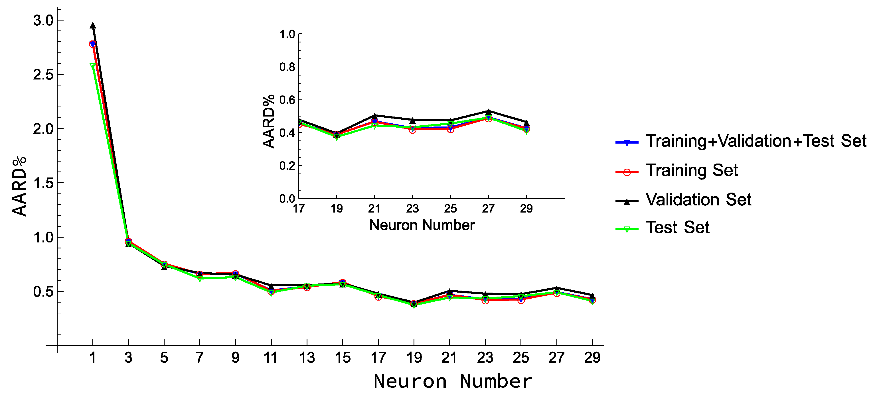
In this study, to avoid overfitting the proposed network, we chose to split the entire dataset as follows: the training set comprised 80% of the data, the validation set contained 10%, and the remaining 10% was used for the test set. Table 1 details the number of points. Another way to avoid overfitting is by using a network with few neurons with a lean and non-rigid architecture. For this reason, it was chosen to design a network with only 1 hidden layer and 19 neurons. As shown in Figure 2, the ANN with 19 neurons ensured excellent results, which are summarized in Table 3. The same table reports additional statistical parameters that characterize the various datasets. The average absolute relative deviation (AARD%), maximum absolute relative deviation (MARD%), and root mean square error (RMSE) were compared:
A A R D % = 100 N i = 1 N | λ i exp λ i calc λ i exp |
M A R D % = M a x ( 100 N i = 1 N | λ i exp λ i calc λ i exp | )
R M S E = 1 N i = 1 N ( λ C a l c . λ E x p ) 2  
As evident in Table 3, all statistical values are aligned, confirming the goodness of the proposed network, which manages to model the thermal conductivity of alternative liquid refrigerants accurately. In particular, the ANN provided very low deviations over the entire database, reaching an AARD% of 0.389%. It is also important to note that the deviations of the test set are aligned with those of the other sets, confirming the prediction capability of the network and the low overfitting tendency. In fact, the test set has an AARD% of 0.375% with a MARD% of 4.598%, in line with the deviations of all other datasets.
Moreover, the K-fold cross-validation technique was used after dividing the dataset into 4 subsets. The model used the first subset in the first iteration to test the model, while the remaining dataset was used to train the model. The second subset helped to test the model, and the other subsets supported the training process. The same procedure was repeated until the test set used every subset. The results are shown in Table 4, in which all the deviations are in line, and there are no particular critical issues in either the test or validation sets.
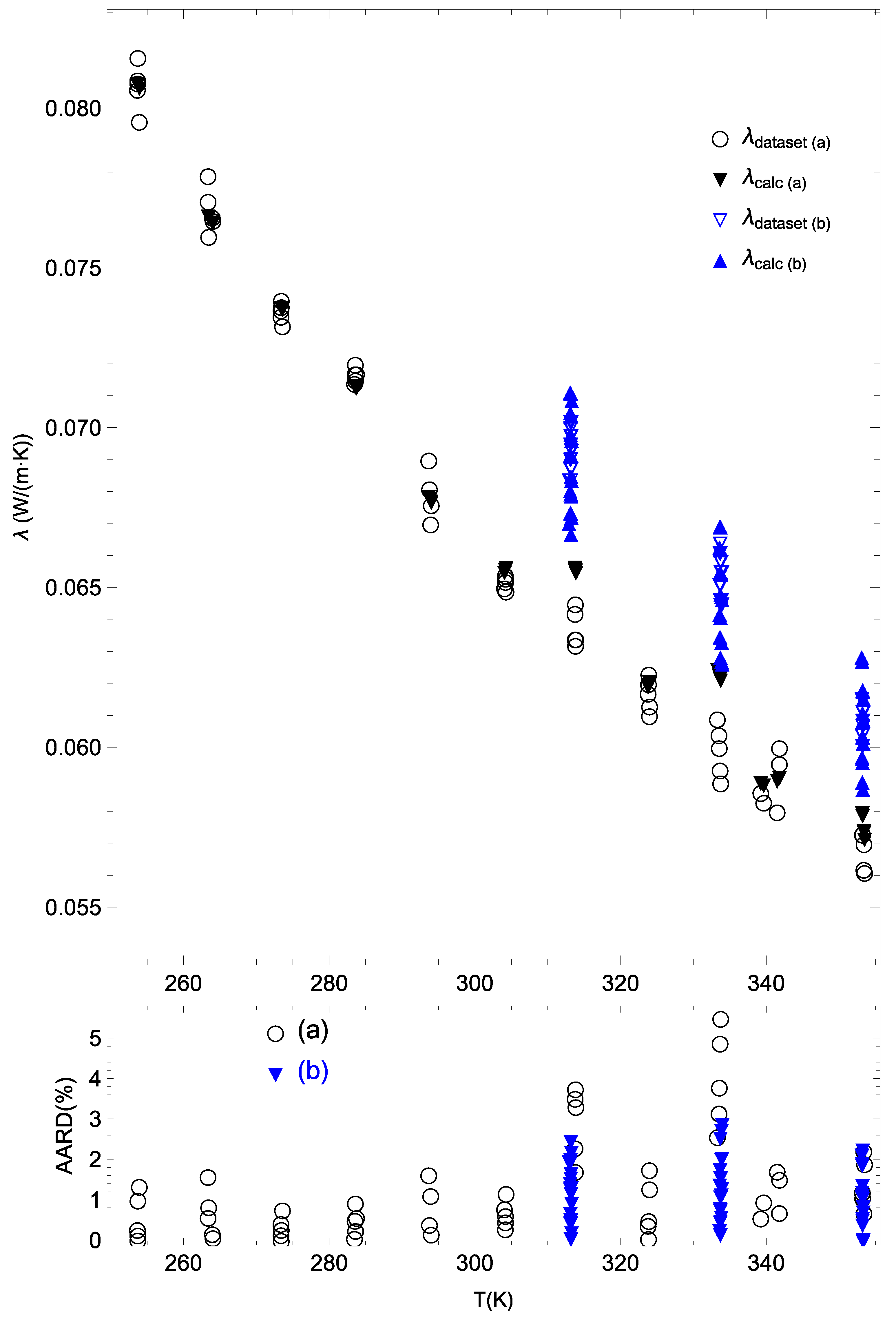
Table 5 shows the AARD% per fluid. Again, homogeneity in the results can be observed. The fluid with the largest deviation is R1336mzz(E), with an AARD% of 1.223% and a MARD% of 5.499%. Figure 3 shows the experimental and calculated conductivity of R1336mzz(E) fluid and the relative deviations. It is evident that the network can accurately reproduce the behavior of liquid thermal conductivity of this refrigerant as a function of the temperature. However, higher deviations can be seen at some specific temperatures. From an in-depth analysis of the results, it was found that this outcome could be due to the different temperature and pressure behaviors of the experimental point provided by the two sources [39,40] presenting λL data for R1336mzz(E).
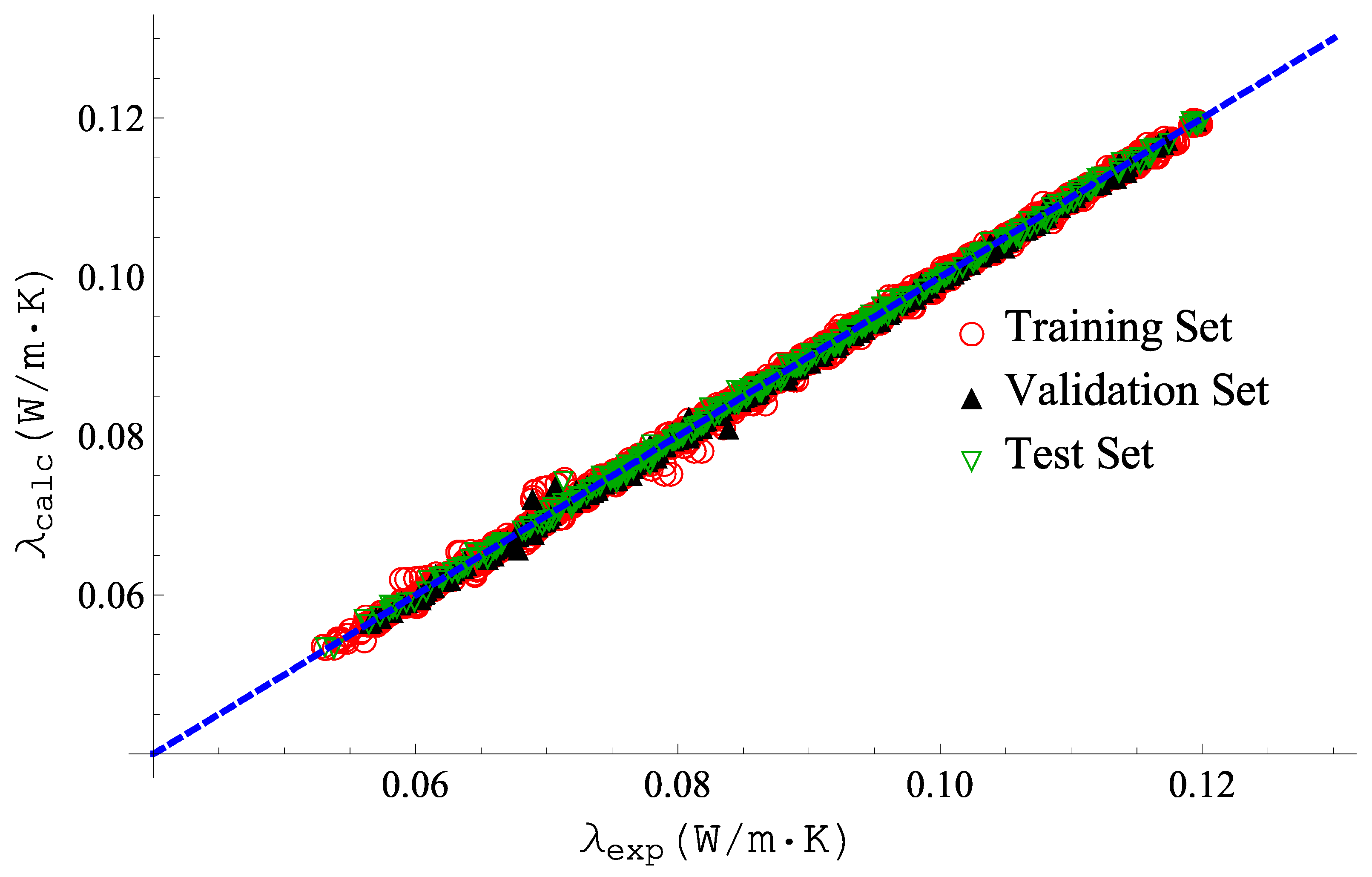
However, the behavior of the entire network is very satisfactory, as can also be seen in Figure 4 where an excellent agreement of the computed points with respect to the experimental data is evident. Furthermore, Figure 4 shows that for the training, validation, and test datasets, the behavior of the network is always close to the bisector of the first and third quadrants, demonstrating the good performance of the network architecture.
The deviations provided using the proposed neural network were compared with that given using Equation (1) and the models used in REFPROP 10.0. The results of these models are also reported in Table 5. The results for R1336mmz(E) provided by REFPROP 10.0 are not reported in this table since a model to calculate its thermal conductivity is currently not available in the software. This table shows that the proposed ANN ensured the lowest AARD% for all the studied low-GWP refrigerants, while REFPROP 10.0 gave the highest overall AARD% for the complete dataset. This outcome is due to high deviations obtained for R1224yd(Z) and R1336mzz(Z), for which preliminary models for thermal conductivity are available in the software. Instead, REFPROP 10.0 ensured accurate results for the other selected fluids. Despite its simplicity, Equation (1) generally provided good results. As expected, this correlation gave higher deviations for R1336mmz(E) since its λL data were not used in the regression of the coefficients.
A direct comparison between the results of the neural network and that of Equations (2) and (3) is not presented since it was not possible to compare the complete dataset with the calculations of the two models. In fact, Equation (2) needs the density as an input, but this property is not available for some of the studied refrigerants. Instead, Equation (3) can be used only to calculate λL along the saturation line.
Finally, it is not trivial to directly compare the results of the neural network presented in this work and that of Wang et al. [26] since they were developed using a different dataset. However, it is worth noting that, for the three common HFOs, i.e., R1234yf, R1234ze(E), and R1336mzz(Z), the presented ANN ensured better results than that of the literature model. The ANN of Wang et al. [26] provided the following AARD%: 1.63% for R1234yf, 4.33% for R1234ze(E), and 0.62% for R1336mzz(Z).

5. Conclusions

In this paper, a feed-forward network was used to describe the liquid thermal conductivity of low-GWP refrigerants. Specifically, the network was trained on a database of 3404 experimental data, achieving excellent results using the entire database. The absolute average relative deviation reached 0.389%, with a maximum absolute relative deviation of 6.074% on the whole dataset. Different methodologies, such as splitting the dataset into different subsets and the K-fold cross-validation technique, were implemented to avoid problems of overfitting and non-predictability of the network. In all cases, it was seen that the network succeeds with an excellent predictive rate on new thermal conductivity points. Moreover, a comparison was made with models from the literature to evaluate the goodness of the algorithm. It was found that the network ensured better results when compared with the following techniques to estimate the liquid thermal conductivity available in the literature: the correlation proposed by Tomassetti et al. [22] and the models used in REFPROP 10.0 [9]. The correlation gave an absolute average relative deviation of 2.585% for the complete dataset. Instead, the software provided an absolute average relative deviation of 3.820% for six refrigerants. Finally, it is worth remarking that the proposed neural network is more complex than many correlations available in the literature; therefore, it should be used only when high accuracy is required. In addition, it is not ensured that the proposed network could provide accurate values for the liquid thermal conductivity of low-GWP refrigerants that were not considered in its development.

Author Contributions

Conceptualization, M.P.; Methodology, M.P., S.T. and G.D.N.; Data curation, S.T.; Writing—original draft, M.P. and S.T.; Writing—review & editing, M.P., S.T. and G.D.N. All authors have read and agreed to the published version of the manuscript.

Funding

This research received no external funding.

Data Availability Statement

No new data were created or analyzed in this study. Data sharing is not applicable to this article.

Conflicts of Interest

The authors declare no conflict of interest.

References

  1. Regulation, E. No 517/2014 of the European Parliament and the Council of 16 April 2014 on Fluorinated Greenhouse Gases and Repealing Regulation (EC) No 842/2006. 2014. Available online: http//eur-lex.Eur.eu/legal-content/EN/TXT/PDF (accessed on 15 May 2016).
  2. UNEP. Amendment to the Montreal Protocol on Substances that Deplete the Ozone Layer (Kigali Amendment). Int. Leg. Mater. 2017, 56, 193–205. [Google Scholar] [CrossRef] [Green Version]
  3. McLinden, M.O.; Huber, M.L. (R) Evolution of refrigerants. J. Chem. Eng. Data 2020, 65, 4176–4193. [Google Scholar] [CrossRef] [PubMed]
  4. McLinden, M.O.; Brown, J.S.; Brignoli, R.; Kazakov, A.F.; Domanski, P.A. Limited options for low-global-warming-potential refrigerants. Nat. Commun. 2017, 8, 14476. [Google Scholar] [CrossRef] [PubMed] [Green Version]
  5. Domanski, P.A.; Brignoli, R.; Brown, J.S.; Kazakov, A.F.; McLinden, M.O. Low-GWP refrigerants for medium and high-pressure applications. Int. J. Refrig. 2017, 84, 198–209. [Google Scholar] [CrossRef]
  6. Uddin, K.; Saha, B.B. An Overview of Environment-Friendly Refrigerants for Domestic Air Conditioning Applications. Energies 2022, 15, 8082. [Google Scholar] [CrossRef]
  7. Uddin, K.; Saha, B.B.; Thu, K.; Koyama, S. Low GWP refrigerants for energy conservation and environmental sustainability. In Advances in Solar Energy Research; Springer: Berlin/Heidelberg, Germany, 2019; pp. 485–517. [Google Scholar]
  8. Poling, B.E.; Prausnitz, J.M.; O’Connell, J.P. The Properties of Gases and Liquids, 5th ed.; McGraw-Hill: New York, NY, USA, 2001; ISBN 9780070116825. [Google Scholar]
  9. Huber, M.L. Models for Viscosity, Thermal Conductivity, and Surface Tension of Selected Pure Fluids as Implemented in REFPROP v10.0; National Institute of Standards and Technology: Gaithersburg, MD, USA, 2018.
  10. Kang, K.; Li, X.; Gu, Y.; Wang, X. Thermal conductivity prediction of pure refrigerants and mixtures based on entropy-scaling concept. J. Mol. Liq. 2022, 368, 120568. [Google Scholar] [CrossRef]
  11. Yang, X.; Kim, D.; May, E.F.; Bell, I.H. Entropy Scaling of Thermal Conductivity: Application to Refrigerants and Their Mixtures. Ind. Eng. Chem. Res. 2021, 60, 13052–13070. [Google Scholar] [CrossRef]
  12. Fouad, W.A.; Vega, L.F. Transport properties of HFC and HFO based refrigerants using an excess entropy scaling approach. J. Supercrit. Fluids 2018, 131, 106–116. [Google Scholar] [CrossRef]
  13. Liu, H.; Yang, F.; Yang, X.; Yang, Z.; Duan, Y. Modeling the thermal conductivity of hydrofluorocarbons, hydrofluoroolefins and their binary mixtures using residual entropy scaling and cubic-plus-association equation of state. J. Mol. Liq. 2021, 330, 115612. [Google Scholar] [CrossRef]
  14. Khosharay, S.; Khosharay, K.; Di Nicola, G.; Pierantozzi, M. Modelling investigation on the thermal conductivity of pure liquid, vapour, and supercritical refrigerants and their mixtures by using Heyen EOS. Phys. Chem. Liq. 2018, 56, 124–140. [Google Scholar] [CrossRef]
  15. Niksirat, M.; Aeenjan, F.; Khosharay, S. Introducing hydrogen bonding contribution to the Patel-Teja thermal conductivity equation of state for hydrochlorofluorocarbons, hydrofluorocarbons and hydrofluoroolefins. J. Mol. Liq. 2022, 351, 118631. [Google Scholar] [CrossRef]
  16. Liu, Y.; Wu, C.; Zheng, X.; Li, Q. Modeling thermal conductivity of liquid hydrofluorocarbon, hydrofluoroolefin and hydrochlorofluoroolefin refrigerants. Int. J. Refrig. 2022, 140, 139–149. [Google Scholar] [CrossRef]
  17. Di Nicola, G.; Coccia, G.; Tomassetti, S. A modified Kardos equation for the thermal conductivity of refrigerants. J. Theor. Comput. Chem. 2018, 17, 1850012. [Google Scholar] [CrossRef]
  18. Yang, S.; Tian, J.; Jiang, H. Corresponding state principle based correlation for the thermal conductivity of saturated refrigerants liquids from Ttr to 0.90 Tc. Fluid Phase Equilibria 2020, 509, 112459. [Google Scholar] [CrossRef]
  19. Latini, G.; Sotte, M. Refrigerants of the methane, ethane and propane series: Thermal conductivity calculation along the saturation line. Int. J. Air-Cond. Refrig. 2011, 19, 37–43. [Google Scholar] [CrossRef] [Green Version]
  20. Latini, G.; Sotte, M. Thermal conductivity of refrigerants in the liquid state: A comparison of estimation methods. Int. J. Refrig. 2012, 35, 1377–1383. [Google Scholar] [CrossRef]
  21. Di Nicola, G.; Ciarrocchi, E.; Coccia, G.; Pierantozzi, M. Correlations of thermal conductivity for liquid refrigerants at atmospheric pressure or near saturation. Int. J. Refrig. 2014, 45, 168–176. [Google Scholar] [CrossRef]
  22. Tomassetti, S.; Coccia, G.; Pierantozzi, M.; Di Nicola, G. Correlations for liquid thermal conductivity of low GWP refrigerants in the reduced temperature range 0.4 to 0.9 from saturation line to 70 MPa. Int. J. Refrig. 2020, 117, 358–368. [Google Scholar] [CrossRef]
  23. Rykov, S.V.; Kudryavtseva, I. V Heat Conductivity of Liquid Hydrofluoroolefins and Hydrochlorofluoroolefins on the Line of Saturation. Russ. J. Phys. Chem. A 2022, 96, 2098–2104. [Google Scholar] [CrossRef]
  24. Pierantozzi, M.; Petrucci, G. Modeling thermal conductivity in refrigerants through neural networks. Fluid Phase Equilibria 2018, 460, 36–44. [Google Scholar] [CrossRef]
  25. Ghaderi, F.; Ghaderi, A.H.; Ghaderi, N.; Najafi, B. Prediction of the thermal conductivity of refrigerants by computational methods and artificial neural network. Front. Chem. 2017, 5, 99. [Google Scholar] [CrossRef] [PubMed] [Green Version]
  26. Wang, X.; Li, Y.; Yan, Y.; Wright, E.; Gao, N.; Chen, G. Prediction on the viscosity and thermal conductivity of hfc/hfo refrigerants with artificial neural network models. Int. J. Refrig. 2020, 119, 316–325. [Google Scholar] [CrossRef]
  27. Ogedjo, M.; Kapoor, A.; Kumar, P.S.; Rangasamy, G.; Ponnuchamy, M.; Rajagopal, M.; Banerjee, P.N. Modeling of sugarcane bagasse conversion to levulinic acid using response surface methodology (RSM), artificial neural networks (ANN), and fuzzy inference system (FIS): A comparative evaluation. Fuel 2022, 329, 125409. [Google Scholar] [CrossRef]
  28. Khamparia, A.; Pandey, B.; Pandey, D.K.; Gupta, D.; Khanna, A.; de Albuquerque, V.H.C. Comparison of RSM, ANN and Fuzzy Logic for extraction of Oleonolic Acid from Ocimum sanctum. Comput. Ind. 2020, 117, 103200. [Google Scholar] [CrossRef]
  29. Latini, G.; Nicola, G.D.; Pierantozzi, M.; Coccia, G.; Tomassetti, S. Artificial Neural Network Modeling of Liquid Thermal Conductivity for alkanes, ketones and silanes. Proc. J. Phys. Conf. Ser. 2017, 923, 012054. [Google Scholar] [CrossRef] [Green Version]
  30. Mulero, Á.; Pierantozzi, M.; Cachadiña, I.; Di Nicola, G. An Artificial Neural Network for the surface tension of alcohols. Fluid Phase Equilibria 2017, 449, 28–40. [Google Scholar] [CrossRef]
  31. Hosseini, S.M.; Pierantozzi, M.; Moghadasi, J. Viscosities of some fatty acid esters and biodiesel fuels from a rough hard-sphere-chain model and artificial neural network. Fuel 2019, 235, 1083–1091. [Google Scholar] [CrossRef]
  32. Alam, M.J.; Yamaguchi, K.; Hori, Y.; Kariya, K.; Miyara, A. Measurement of thermal conductivity and viscosity of cis-1-chloro-2, 3, 3, 3-tetrafluoropropene (R-1224yd (Z)). Int. J. Refrig. 2019, 104, 221–228. [Google Scholar] [CrossRef]
  33. Perkins, R.A.; Huber, M.L.; Assael, M.J. Measurement and Correlation of the Thermal Conductivity of trans-1-Chloro-3, 3, 3-trifluoropropene (R1233zd (E)). J. Chem. Eng. Data 2017, 62, 2659–2665. [Google Scholar] [CrossRef]
  34. Alam, M.J.; Islam, M.A.; Kariya, K.; Miyara, A. Measurement of thermal conductivity and correlations at saturated state of refrigerant trans-1-chloro-3, 3, 3-trifluoropropene (R-1233zd (E)). Int. J. Refrig. 2018, 90, 174–180. [Google Scholar] [CrossRef]
  35. Perkins, R.A.; Huber, M.L. Measurement and Correlation of the Thermal Conductivity of 2, 3, 3, 3-Tetrafluoroprop-1-ene (R1234yf) and trans-1, 3, 3, 3-Tetrafluoropropene (R1234ze (E)). J. Chem. Eng. Data 2011, 56, 4868–4874. [Google Scholar] [CrossRef]
  36. Miyara, A.; Fukuda, R.; Tsubaki, K. Thermal conductivity of saturated liquid of R1234ze (E)+ R32 and R1234yf+ R32 mixtures. Trans. Jpn. Soc. Refrig. Air Cond. Eng. 2011, 28, 435–443. [Google Scholar]
  37. Miyara, A.; Tsubaki, K.; Sato, N.; Fukuda, R. Thermal conductivity of saturated liquid HFO-1234ze (E) and HFO-1234ze (E)+ HFC-32 mixture. In Proceedings of the 23rd IIR International Congress of Refrigeration, Prague, Czech Republic, 21–26 August 2011. [Google Scholar]
  38. Ishida, H.; Mori, S.; Kariya, K.; Miyara, A. Thermal conductivity measurements of low GWP refrigerants with hot-wire method. In Proceedings of the 24th International Congress of Refrigeration (ICR), Yokohama, Japan, 16–22 August 2015. [Google Scholar]
  39. Mondal, D.; Kariya, K.; Tuhin, A.R.; Miyoshi, K.; Miyara, A. Thermal conductivity measurement and correlation at saturation condition of HFO refrigerant trans-1, 1, 1, 4, 4, 4-hexafluoro-2-butene (R1336mzz (E)). Int. J. Refrig. 2021, 129, 109–117. [Google Scholar] [CrossRef]
  40. Haowen, G.; Xilei, W.; Yuan, Z.; Zhikai, G.; Xiaohong, H.; Guangming, C. Experimental and Theoretical Research on the Saturated Liquid Thermal Conductivity of HFO-1336mzz (E). Ind. Eng. Chem. Res. 2021, 60, 9592–9601. [Google Scholar] [CrossRef]
  41. Perkins, R.A.; Huber, M.L. Measurement and Correlation of the Thermal Conductivity of cis-1, 1, 1, 4, 4, 4-hexafluoro-2-butene. Int. J. Thermophys. 2020, 41, 103. [Google Scholar] [CrossRef]
  42. Alam, M.J.; Islam, M.A.; Kariya, K.; Miyara, A. Measurement of thermal conductivity of cis-1, 1, 1, 4, 4, 4-hexafluoro-2-butene (R-1336mzz (Z)) by the transient hot-wire method. Int. J. Refrig. 2017, 84, 220–227. [Google Scholar] [CrossRef]
  43. Akasaka, R.; Fukushima, M.; Lemmon, E.W. A Helmholtz Energy Equation of State for cis-1-chloro-2, 3, 3, 3-tetrafluoropropene (R-1224yd (Z)). In Proceedings of the European Conference on Thermophysical Properties, Graz, Austria, 3–8 September 2017. [Google Scholar]
  44. Richter, M.; McLinden, M.O.; Lemmon, E.W. Thermodynamic Properties of 2,3,3,3-Tetrafluoroprop-1-ene (R1234yf): Vapor Pressure and p–ρ–T Measurements and an Equation of State. J. Chem. Eng. Data 2011, 56, 3254–3264. [Google Scholar] [CrossRef]
  45. Thol, M.; Lemmon, E.W. Equation of State for the Thermodynamic Properties of trans-1, 3, 3, 3-Tetrafluoropropene [R-1234ze (E)]. Int. J. Thermophys. 2016, 37, 28. [Google Scholar] [CrossRef]
  46. Akasaka, R.; Lemmon, E.W. Fundamental Equations of State for cis-1, 3, 3, 3-Tetrafluoropropene [R-1234ze (Z)] and 3, 3, 3-Trifluoropropene (R-1243zf). J. Chem. Eng. Data 2019, 64, 4679–4691. [Google Scholar] [CrossRef]
  47. Tanaka, K.; Ishikawa, J.; Kontomaris, K.K. Thermodynamic properties of HFO-1336mzz (E)(trans-1, 1, 1, 4, 4, 4-hexafluoro-2-butene) at saturation conditions. Int. J. Refrig. 2017, 82, 283–287. [Google Scholar] [CrossRef]
  48. Lemmon, E.W.; Bell, I.H.; Huber, M.L.; McLinden, M.O. NIST Standard Reference Database 23: Reference Fluid Thermodynamic and Transport Properties-REFPROP, Version 10.0, National Institute of Standards and Technology, 2018. 2018. Available online: http//www.nist.gov/srd/nist23.cfm (accessed on 25 October 2022).
  49. Sakoda, N.; Higashi, Y. Measurements of PvT Properties, Vapor Pressures, Saturated Densities, and Critical Parameters for cis-1-Chloro-2, 3, 3, 3-tetrafluoropropene (R1224yd (Z)). J. Chem. Eng. Data 2019, 64, 3983–3987. [Google Scholar] [CrossRef]
  50. Basheer, I.A.; Hajmeer, M. Artificial neural networks: Fundamentals, computing, design, and application. J. Microbiol. Methods 2000, 43, 3–31. [Google Scholar] [CrossRef] [PubMed]
  51. Krogh, A. What are artificial neural networks? Nat. Biotechnol. 2008, 26, 195–197. [Google Scholar] [CrossRef] [PubMed]
  52. Bishop, C.M. Neural networks and their applications. Rev. Sci. Instrum. 1994, 65, 1803–1832. [Google Scholar] [CrossRef]
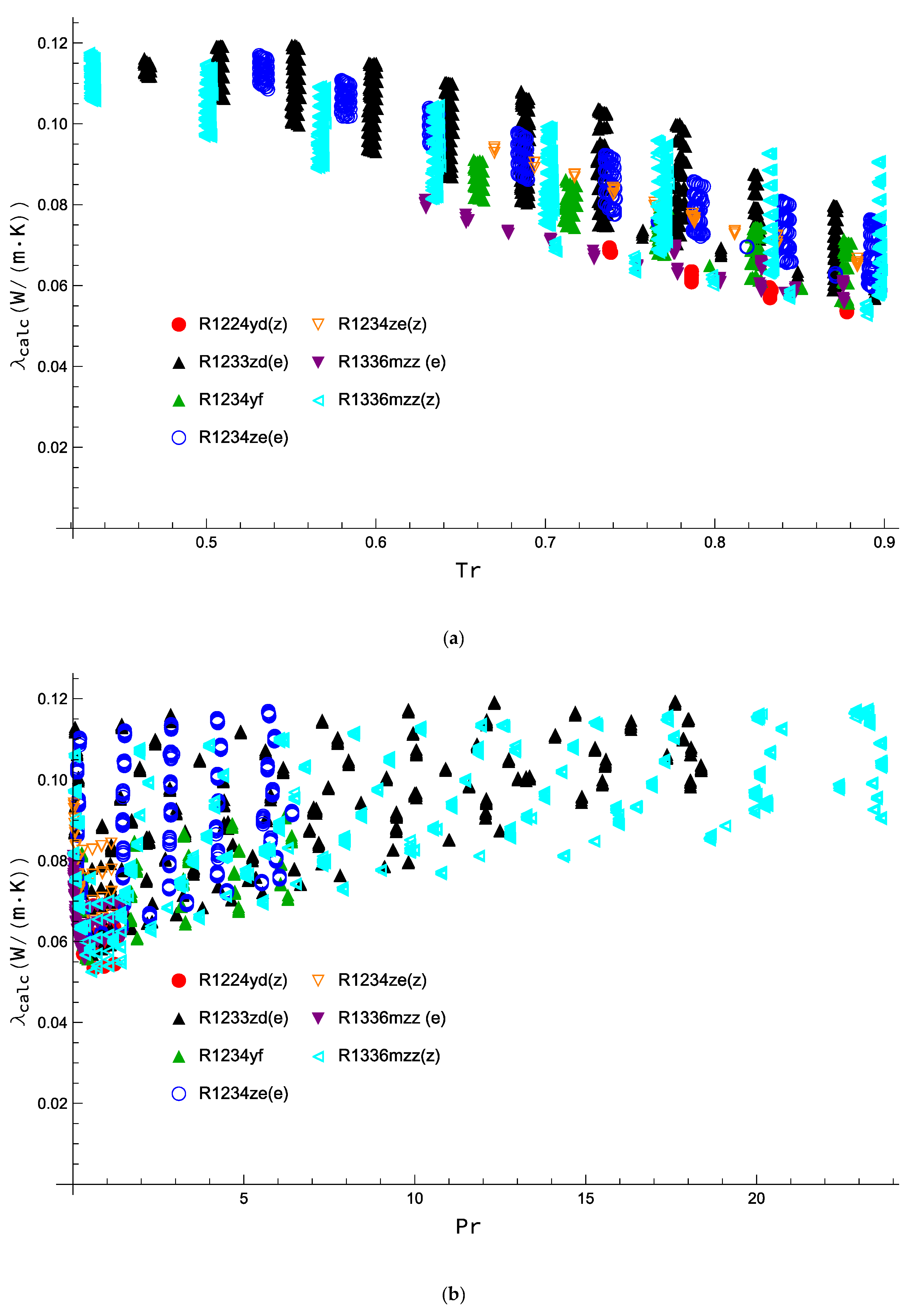
Figure 1. Liquid thermal conductivity behavior of the analyzed halogenated alkene refrigerants as a function of the reduced temperature (a) and the reduced pressure (b).
Applsci 13 00260 g001
Figure 2. Absolute average percent deviation between data collected and the ANN results vs. the number of neurons in the hidden layer.
Applsci 13 00260 g002
Figure 3. Behavior of R1336mzz(E) and absolute relative average percent deviation related to experimental temperature. (a) corresponds to Ref. [40] and (b) corresponds to Ref. [39].
Applsci 13 00260 g003
Figure 4. Correlation between the experimental and the corresponding calculated thermal conductivity data divided into the training, validation, and test sets.
Applsci 13 00260 g004
Table 3. Statistical parameters for the individual datasets including the training set, validation set, test set, and the entire dataset.
Data SetPoint N.AARD%MARD%RMSE
Training set27230.3906.0740.0005
Validation Set3400.3964.9450.0005
Test Set3410.3754.5980.0005
Overall34040.3892.0700.0003
Table 4. Performance of the ANN using a 4-fold cross-validation procedure.
ModelTraining Set
Point N.
Test Set
Point N.
Training Set AARD%
RMSE
Test Set
AARD%
RMSE
Cross Validation 125538510.557
0.0007
0.643
0.0022
Cross Validation 225538510.904
0.0011
0.853
0.0026
Cross Validation 325538510.354
0.0004
0.932
0.0032
Cross Validation 425538510.417
0.0005
1.087
0.0032
Table 5. Average absolute relative and maximum absolute relative deviations between the experimental λL data of the studied refrigerants and the calculations provided by the proposed neural network, Equation (1) and REFPROP 10.0.
Fluid NameN. of
Points
This WorkEquation (1)REFPROP 10.0
AARD%MARD%AARD%MARD%AARD%MARD%
R1224yd(Z)530.4511.2993.0415.8966.3658.861
R1233zd(E)11320.2601.5451.1553.9300.3371.584
R1234yf2670.2901.1631.4467.2420.3031.557
R1234ze(E)4940.2512.2351.6345.9410.3362.041
R1234ze(Z)610.5601.5741.7715.0801.7755.705
R1336mzz(E)1181.2235.4996.45613.197--
R1336mzz(Z)12790.4906.0744.12019.0189.39013.84
Overall34040.389-2.585-3.82-
Disclaimer/Publisher’s Note: The statements, opinions and data contained in all publications are solely those of the individual author(s) and contributor(s) and not of MDPI and/or the editor(s). MDPI and/or the editor(s) disclaim responsibility for any injury to people or property resulting from any ideas, methods, instructions or products referred to in the content.