An Efficient Prediction System for Coronary Heart Disease Risk Using Selected Principal Components and Hyperparameter Optimization

Abstract

Medical science-related studies have reinforced that the prevalence of coronary heart disease which is associated with the heart and blood vessels has been the most significant cause of health loss and death globally. Recently, data mining and machine learning have been used to detect diseases based on the unique characteristics of a person. However, these techniques have often posed challenges due to the complexity in understanding the objective of the datasets, the existence of too many factors to analyze as well as lack of performance accuracy. This research work is of two-fold effort: firstly, feature extraction and selection. This entails extraction of the principal components, and consequently, the Correlation-based Feature Selection (CFS) method was applied to select the finest principal components of the combined (Cleveland and Statlog) heart dataset. Secondly, by applying datasets to three single and three ensemble classifiers, the best hyperparameters that reflect the pre-eminent predictive outcomes were investigated. The experimental result reveals that hyperparameter optimization has improved the accuracy of all the models. In the comparative studies, the proposed work outperformed related works with an accuracy of 97.91%, and an AUC of 0.996 by employing six optimal principal components selected from the CFS method and optimizing parameters of the Rotation Forest ensemble classifier.

1. Introduction

1.1. Motivation and Background

Coronary Heart Disease (CHD) occurs when the heart’s arteries are unable to supply the heart with adequate oxygen-rich blood; thus, making it one of the most complicated diseases to treat. Among the cause attributed to coronary complication is plaque; a waxy substance that gets deposited inside the lining of major coronary arteries and, over time, partially or completely obstructs blood flow into the arteries [1,2]. CHD is often classified as a silent killer as many people do not realize that they have CHD until they have chest discomfort, a heart attack, or sudden cardiac arrest because they have no symptoms. Hence, early detection is thus a high priority to provide needful advice and if necessary, ensure effective medical care [3,4]. CHDs are the leading cause of death worldwide, claiming the lives of an estimated 17.9 million people annually. Heart attacks and strokes account for more than four out of every five CHD deaths, with one-third of these deaths occurring before age 70 [5].

Several factors have been recognized as risk variables for coronary heart disease through medical and clinical studies. These are categorized into two groups. The first group of risk variables comprises those that cannot be changed, such as age, gender, and family history [6]. The second group includes those that can be altered, such as nicotine consumption, undue alcohol intake, dietary habits, extreme cholesterol, overweight, and physical inactivity [7,8]. Subsequently, these risk variables can be eliminated or reduced by altering one’s lifestyle and taking appropriate medication [9]. CHD diagnosis is difficult, specifically in developing and underdeveloped countries where qualified expertise and equipment are scarce [10]. However, it is acknowledged that CHD diagnostic task is a challenging process which involves a careful review of the patient’s medical history, a heart specialist assessment of various symptoms, and physical cross-examination report [11,12]. Due to the complexity of the process, inaccurate detection or delays in clinical treatment might lead to an increase in health loss and mortality, thus the implementation of an automated and intelligent coronary heart disease risk prediction model that is efficient is highly desirable [13].

With the massive amounts of patient data that have been available in recent years, the diagnosis of CHD may now be done automatically using statistical approaches to predict the likelihood of each patient having this chronic disease. In this connection, Machine learning (ML) offers a significant impact as an analytical technique to improve prediction results in many applications [14,15,16,17,18,19,20,21], especially of heart disease risk [22,23,24]. As an overview, the ML mechanism is dependent on data that are provided to the machine (training sets) for which disease status (disease or no disease) is known. The next stage involves applying the outcome of this algorithm to a variable dataset to predict the disease status and consequently potentially minimize required clinical intervention [25,26,27]. Data mining-based CHD prediction systems could help doctors make accurate prognostications based on patient clinical data [28]. Feature selection is efficient for prediction performance and is vital in many real-world applications, particularly in medical diagnostics, where physicians, doctors, and medical experts can investigate the most important symptoms that have a substantial influence on the likelihood of developing the disease [29,30].

1.2. Purpose, Contribution, and Paper Structure

This research work aims to implement an unconventional method of feature extraction and feature selection on a combined Cleveland and Statlog heart datasets to improve the result of coronary heart disease risk prediction. As an initial stage, the principal components of the combined heart dataset were determined, and then, the best principal components were obtained by applying the Correlation-based Feature Selection (CFS) method with the Best First search procedure. Thenceforth, the single and ensemble machine learning algorithms were trained on full and selected principal components. This entails the hyperparameter optimization analysis to attain the best hyperparameters that impact the performance of the classifiers significantly in view of improving the prediction outcomes.

The key contributions of this research work are summarized as follows:

• An accurate coronary heart risk prediction system has been developed based on selected principal components and machine learning algorithms.
• The impact of selecting significant principal components using the CFS technique to improve the prediction results for heart disease diagnosis by reducing the training time has been investigated.
• The performance of the single classifiers such as Decision Tree (DT), Support Vector Machines (SVM), K-Nearest Neighbors (KNN), and ensemble classifiers including AdaBoost M1 (AB), Bagging (BG), and Rotation Forest (RTF) has been examined with and without hyperparameter optimization.
• A performance comparison of state-of-the-art works on coronary heart disease risk prediction with the proposed method has been provided.

The rest of the paper is organized as follows: Section 2 details the related works, and Section 3 focuses on materials and methods. Results and analysis are detailed in Section 4; a discussion is provided in Section 5. Finally, the conclusion and future work is given in Section 6.

2. Related Works

This section discusses the most up-to-date approaches for detecting coronary heart disease using machine learning algorithms, as demonstrated by numerous successful research studies. A summary of related works is provided in Table 1.

Table 1. Summary of the related works.

No.	Author(s) & Year	Feature Selection (FS), Classifiers Trained, & Validation Method	Performance Metrics & Software (SW)	Remarks
1.	Javeed et al. [31], 2019	FS: Random search algorithm Classifiers: RF Hold-out (70:30) validation	Accuracy, sensitivity, specificity, MCC, and ROC-AUC SW: Python programming	Only one classifier has been trained and the dataset samples become fewer when using hold-out validation.
2.	Alam et al. [32], 2019	FS: InfoGain, GainRatio, Correlation, OneR, and ReliefF Classifiers: RF 10-fold cross-validation (CV)	Accuracy and AUC SW: Weka	One classifier has been utilized and the accuracy achieved was a moderate value.
3.	Mohamed et al. [33], 2019	FS: Parasitism-predation algorithm Classifiers: KNN with 10-fold CV	Accuracy and execution time SW: Matlab 2017a	Only one classifier has been trained and achieved moderate accuracy.
4.	Pasha et al. [34], 2020	FS: Novel feature reduction Classifiers: LR, RF, BRT, SGB, and SVM Hold-out (70:30) validation	Accuracy and AUC SW: R programming	Dataset samples were lesser with the 70:30 train-test split resulting in high variance.
5.	Saqlain et al. [35], 2019	FS: MFSFSA, FFSA, RFSA Classifiers: RBF SVM with 10-fold CV	Accuracy, sensitivity, and specificity SW: not specified	Only one classifier has been trained and the accuracy achieved was poor.
6.	Bharti et al. [36], 2021	FS: LASSO Classifiers: LR, KNN, SVM, RF, DT, and DL with 10-fold cross-validation	Accuracy, specificity, and sensitivity SW: Python programming	Achieved good accuracy of 94.2%. However, the specificity and sensitivity are poor.
7.	Muhammad et al. [37], 2020	FS: FCBF, mRMR, LASSO, and Relief Classifiers: KNN, DT, Extra-Tree (ET), RF, LR, NB, ANN, SVM, AdaBoost, and GB with 10-fold cross-validation	Accuracy, Sensitivity, Specificity, AUC, Precision, F1-Score, MCC SW: Python programming	ET classifier provided 92.09% of accuracy with full features, and 94.41% with Relief FS.
8.	Ali et al. [38], 2019	FS: Chi-square Classifiers: Optimized deep neural network	Accuracy, specificity, sensitivity, MCC, and AUC SW: Python programming	Though sensitivity is 100%, the accuracy is about 7% less than that.
9.	Kanagarathinam et al. [39], 2022	FS: Pearson’s correlation coefficient Classifiers: NB, XGBoost, k-NN, SVM, MLP, and CatBoost 10-fold cross-validation, 80:20 train-test	Accuracy and AUC SW: Python programming	With the CatBoost classifier achieved 94.34% of accuracy, whereas other classifiers underperformed.
10.	Gupta et al. [40], 2022	Classifiers: LR, SVM, NB, DT, KNN, and RF 70:30 train-test split	Accuracy, sensitivity, specificity, precision, and F1 score SW: Python programming	No feature selection method was employed. Lesser number of observations for validating the model.
11.	Saboor et al. [41], 2022	Classifiers: AB, LR, ET, MNB, CART, SVM, LDA, RF, and XGB.10-fold cross-validation	Accuracy, precision, recall, and F measure SW: Python programming	Achieved better accuracy value by performing hyperparameter tuning but no feature selection technique has been applied.
12.	Chang et al. [42], 2022	FS: Correlation Classifiers: KNN, DT, SVM, RF and LR 10-fold cross-validation	Accuracy SW: Python programming	The achieved accuracy was not up to the level.
13.	Krittanawong (2020), [43]	Classifiers: CNN, SVM, Boosting, RF, DT	AUC, Sensitivity, and Specificity SW: R version 3.2.3	AUC of 0.93 for CAD with custom-built, and 0.92 for Stroke with SVM.
14.	Alaa et al. (2019), [44]	Ensemble of 3 pipelines using AutoPrognosis with RF, XGBoost, NN etc.	AUC-ROC SW: Python programming	The cholesterol biomarkers were not included. Feature selection has not been employed in this work.
15.	Joloudari et al. (2020), [45]	FS: RTs, DT, CHAID, and SVM Classifier: RTs, DT, CHAID, and SVM with 10-fold CV	Accuracy and AUC SW: IBM Spss Modeler 18.0	Unbalanced dataset and the methods used for attribute ranking also used for classification task.
16.	Baccouche et al. (2020), [46]	FS: Model-based and Recursive feature elimination Classifiers: Ensemble Deep learning80:20 train-test ratio	Accuracy and F1-Score SW: Python programming	The methodology is computationally expensive and does not validate on benchmark datasets.

Javeed et al. [31] developed an efficient and less complex model to increase coronary heart disease risk prediction on the Cleveland dataset using a random search algorithm (RSA) and Random Forest (RF) model. The dataset was split into 70% for training and 30% for testing to evaluate the model. The model achieved an accuracy of 93.33% using a subset of 7 features that accounted for a 3.3% improvement compared to standard RF. The AUC of 0.947 is obtained with the improved version of the RSA-RF model. Alam et al. [32] proposed a ranking-based feature selection method for medical data classification. The RF classifier with 10-fold cross-validation was implemented on the selected ten distinct disease datasets, including Statlog heart data. The feature ranking methods such as Information Gain, Gain Ratio, Correlation, OneR, and Relief attribute evaluators were utilized from the Weka tool. It can be concluded that the RF with 12 attributes selected from the Relief method (excluding feature ‘chol’) performed better than other techniques. It achieved 85.5% of accuracy and an AUC of 0.915.

Mohamed et al. [33] developed a meta-heuristic technique called Parasitism-Predation Algorithms (PPA) for selecting feature subsets to improve the classification accuracy by combining cat swarm optimization (CSO), cuckoo search (CS), and crow search algorithm (CSA). The PPA achieved an accuracy of 86.17% in 49.13 s when the KNN classifier was applied to the selected four features extracted from the Statlog heart dataset using 10-fold cross-validation. Pasha et al. [34] proposed a novel feature reduction (NFR) model for effective heart disease risk prediction on Cleveland, Hungarian, Statlog, and Switzerland datasets. The missing values have been replaced with a mean value of the column, and 70:30 hold-out validation is applied. The performance of Logistic Regression (LR), RF, boosted regression tree (BRT), stochastic gradient boosting (SGB), and SVM algorithms were evaluated by reducing the features based on various subset combinations with maximum accuracies, AUC values, and the slightest difference between them. The results of the proposed model reported an accuracy of 92.53% and an AUC of 0.9268 using LR (9 features) on the Cleveland dataset.

Saqlain et al. [35] projected a feature subset selection method to improve the cardiovascular risk prediction outcomes using mean fisher score-based feature selection algorithms (MFSFSA), forward feature selection algorithm (FFSA), and reverse feature selection algorithm (RFSA). Feature subsets of four UCI heart datasets, Cleveland, Hungarian, Switzerland, and SPECTF, were obtained and fed to the RBF kernel-based SVM classifier. An accuracy of 81.19% is achieved on the Cleveland dataset with seven attributes. Rohit Bharti et al. [36] discussed three methods (without FS and outlier detection, with FS and no outlier detection, and with FS and outlier detection) in predicting heart disease using machine learning and DL on the UCI heart dataset. They claimed that the third method provided better results than the first two approaches. The least absolute shrinkage and selection operation (LASSO) feature selection technique has been applied to select essential features for heart disease and they trained the dataset using LR, KNN, SVM, RF, and DT classifiers. The KNN method achieved 84.8% accuracy, 77.7% specificity, and 85.0% sensitivity, while the deep learning achieved 94.2% accuracy, 82.3% specificity, and 83.1% sensitivity, respectively.

Muhammad et al. [37] generated an intelligent predictive model for the early diagnosis of heart disease by training various machine learning classifiers on the best features of the Cleveland dataset using 10-fold cross-validation. Four feature selection algorithms, namely fast correlation-based filter (FCBF), minimal redundancy maximal relevance (mRMR), LASSO, and Relief, were applied to obtain the essential and more correlated features. An accuracy of 94.41% was gained with the Extra Tree classifier. Ali et al. [38] used hold-out validation with a 70:30 ratio for training and testing datasets to construct an autonomous diagnostic system for heart disease identification employing chi-square feature selection and an improved deep neural network (DNN) for classification on the Cleveland heart dataset. On the test dataset, the proposed hybrid model has an accuracy of 93.33% and an AUC of 0.94.

Kanagarathinam et al. [39] created a dataset named ‘Sathvi’ consisting of 531 observations with 12 features and no missing values by combining the Cleveland, the Hungarian, the Long Beach, and the Switzerland heart datasets. They considered ten features, age, sex, cp, trestbps, chol, fbs, restecg, thalach, exang, and oldpeak, for predicting cardiovascular disease. Redundant features were eliminated using Pearson’s correlation coefficient method. In this work, the ML models were trained using 80.20 hold-out validation, and they achieved an accuracy of 87.85% with the CatBoost algorithm. Further, the CatBoost algorithm has been trained using a 10-fold CV and achieved an accuracy ranging between 88.67% to 98.11%, with a mean accuracy of 94.34%. Gupta et al. [40] developed a machine learning model to identify the risky people suffering from heart disease by splitting the Cleveland heart dataset into a 70:30 ratio for training and testing. The model performed standardization of data to the standard scales and trained various algorithms. It attained the highest accuracy of 92.30% using Logistic Regression. Furthermore, they tuned the KNN classifier with a k value between 2 and 20 and achieved the best accuracy of 90.11% at k = 14. Saboor et al. [41] performed standardization of heart dataset attributes for best prediction results, followed by hyperparameter tuning of machine learning classifiers using the GridSearchCV method to improve the accuracy of heart disease prediction. They evaluated the performance of the classifier models and concluded that the standardization and hyperparameter tuning improved the prediction accuracy. An accuracy of 96.72%, a precision of 98%, a recall of 98%, and an F-measure of 98% were achieved using an SVM classifier with a Sigmoid kernel and complexity parameter, C = 0.5. A similar methodology block diagram proposed by this work is given in Figure 1.

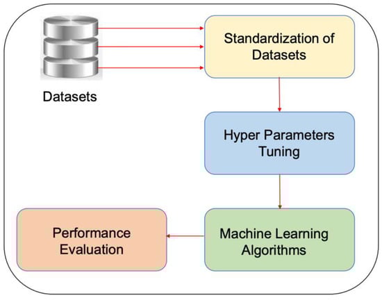
Figure 1. Methodology block diagram.

From Figure 1, the work in [41] has not employed the feature selection to avoid noise or redundant data. Chang et al. [42] developed a python-based application for heart disease detection using the Random Forest algorithm by performing explorative data analysis of heart disease dataset features. The importance of heart dataset attributes using a correlation matrix plot was evaluated, and an accuracy of 83% was achieved in training data.

Krittanawong et al. [43] assessed the predictive ability of machine learning algorithms in CVD. They developed a comprehensive strategy with MEDLINE, Embase, and Scopus databases to predict coronary artery disease (CAD), stroke, heart failure, and cardiac arrhythmias. They achieved an AUC of 0.88, and 0.93 with boosting and custom-built algorithms, respectively, to predict CAD. They obtained an AUC of 0.92, 0.91, 0.90 with SVM, boosting, and CNN algorithms, respectively, to predict stroke. They were not able to provide a confusion matrix for the meta-analytic approach to report all possible evaluation matrices. Alaa et al. [44] developed a machine learning model based on AutoPrognosis to improve heart disease risk prediction with non-traditional variables using UK Biobank (473 variables). They compared the model with Framingham score, and Cox proportional hazards (CoxPH) models in terms of AUC-ROC. They obtained an AUC-ROC of 0.774 compared to that of Framingham score and Cox PH models is 0.724, and 0.734, respectively. The main drawback is that the cholesterol biomarkers were not included in the development of a model.

Joloudari et al. [45] discussed feature selection methods that provide a ranking for the attributes of the dataset to select the best among them in heart disease risk prediction. Several data mining techniques, namely random trees (RTs), decision tree (C5.0), Chi-squared automatic interaction detection (CHAID), and SVM, were utilized to obtain the best-ranked attributes of the Z-Alizadeh Sani heart dataset comprising 303 observations with 55 attributes. An accuracy of 91.47% and AUC of 96.7% have been achieved by selecting 40 attributes with the random tree method. Baccouche et al. [46] proposed an ensemble of deep learning neural networks to classify heart disease patients from the dataset of 800 samples with 141 features collected from Medica Norte Hospital. A comparable ensemble learning model proposed in this work is given in Figure 2.

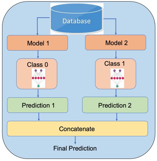
Figure 2. The ensemble learning model.

In Figure 2, model 1 depicts long short-term memory (LSTM), gated recurrent units (GRU), BiLSTM, and BiGRU, and Model 2 is a convolutional neural network (CNN). After performing various preprocessing techniques, the experiments have been carried out with the combination of BiLSTM or BiGRU and CNN. It achieved an accuracy of 96%, and an ACU of 0.99 with BiGRU + CNN by selecting 60 features and tuning the hyperparameters. However, this method necessitates the selection of significant model parameters and more time to train the classification model.

Table 2 provides hyperparameter tuning performed in related works.

Table 2. Hyperparameter tuning performed in related works.

Ref.	Model	Hyperparameters Tuned
[31]	RF	Number of decision trees, E depth of each tree, D
[36]	Deep learning	Dropout layer
[37]	KNN	Number of nearest neighbors, K
	SVM	Kernel
	LR	Regularization strength, C
	ANN	Number of hidden neurons
[38]	DNN	Number of neurons in the first hidden layer, N1 Number of neurons in the second hidden layer, N2
[41]	SVM	Complexity parameter, C and Kernel
[44]	AutoPrognosis	Weighted ML pipelines with XGBoost ensemble (200 estimators)
[46]	Deep learning	Number of epochs, dropout rate, optimizer, learning rate

From the related works, it is understood that selecting significant features in [31,34,37,39] and an ensemble of classifiers as in [31,32,37,39,42,44,46] can substantially enhance the performance of machine learning algorithms in predicting the coronary heart disease risk at an early stage. However, the feature selection is a challenging task as it grows exponentially depending on the number of features in the dataset. The accuracy of the classifiers in predicting coronary heart disease risk varies between 81.19% [35] to 96.72% [41]. Researchers [40,41,43,44] have not employed any feature selection techniques in their works. From Table 2, very few research studies have optimized hyperparameters since tuning numerous ML models in order to identify the optimal hyperparameters is time-consuming. Nonetheless, effective dimensionality reduction and optimization of classifier hyperparameters can increase classifier performance in precisely predicting coronary heart disease risk.

3. Materials and Methods

This section discusses the methodology followed by the description of heart dataset features, data preprocessing, feature extraction, feature selection, machine learning classification, hyperparameter optimization, and performance evaluation. The experimental workflow of the proposed methodology is shown in Figure 3.

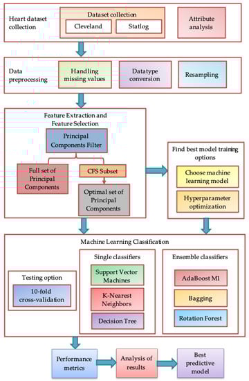
Figure 3. Block diagram of the proposed methodology.

3.1. Proposed Research Methodology

The experimental work is carried out by combining Cleveland and Statlog heart datasets to increase the number of observations. The features with categorical information were then converted from numerical to nominal data types during data preparation, and missing values in the dataset were discovered and data imputation deployed to address them. Subsequently, the principal components of the combined dataset were extracted and the Correlation-based Feature Selection (CFS) method with Best First forward direction search procedure was applied to select the finest principal components of the combined heart dataset. In order to avoid overfitting, resampling of the dataset was carried out. The 10-fold cross-validation technique has been preferred to assess the effectiveness of the machine learning algorithms and various single classifiers such as Support Vector Machines (SVM), K-Nearest Neighbors (KNN), J48 Decision Tree (DT), ensemble classifiers namely, AdaBoost M1 (AB), Bagging (BG), and Rotation Forest (RTF) were trained on the full set of principal components and selected components obtained from the CFS method.

Subsequently, the hyperparameter optimization that enhances the classifier’s performance in predicting coronary heart disease risk was performed to find the best hyperparameters of the classifiers. Finally, the effectiveness of the machine learning models has been assessed by computing the different performance measures using a confusion matrix and a comparative analysis of the anticipated work with the related works has been presented. The metrics accuracy, sensitivity, specificity, precision, and f-measure are calculated as the weighted average of both the target class 0 and 1.

3.2. Dataset Description

The Cleveland dataset [47] with 303 observations and the Statlog [48] with 270 observations from the University of California Irvine (UCI) machine learning repository are combined to yield a total of 573 observations. Table 3 summarizes the characteristics of the merged heart dataset.

Table 3. Description and value range of combined heart dataset attributes.

No.	Attribute	Description and Value Range of Attributes
1.	age	Age of the patients in years (29 to 77)
2.	sex	Gender of the patients (1 = male, 0 = female)
3.	cp	Chest pain type (1—typical angina, 2—atypical angina, 3—non-angina pain, 4—asymptomatic)
4.	trestbps	Resting blood pressure in mm Hg on admission to the hospital (94 to 200)
5.	chol	Serum cholesterol in mg/dl (126 to 564)
6.	fbs	Fasting blood sugar > 120 mg/dl (1—true, 0—false)
7.	restecg	Resting electrocardiographic results (0—normal, 1—ST-T wave abnormality, 2—definite left ventricular hypertrophy)
8.	thalach	Maximum heart rate achieved (71 to 202)
9.	exang	Exercise induces angina (1—yes, 0—no)
10.	oldpeak	ST depression induced by exercise relative to rest (−2.6 to 6.2)
11.	slope	The slope of the peak exercise ST segment (1—upsloping, 2—flat, 3—downsloping)
12.	ca	Number of major vessels colored by fluoroscopy (0–3)
13.	thal	The heart status (3—normal, 6—fixed defect, 7—reversible defect)
14.	target	Prediction attribute (0—absence of heart disease, 1—presence of heart disease)

The attributes with less than ten values, namely ‘sex’, ‘cp’, ‘fbs’, ‘restecg’, ‘exang’, ‘slope’, ‘ca’, thal’, and ‘target’ are classified as nominal or categorical type in Table 3. The leftover attributes ‘age’, ‘trestbps’, ‘chol’, ‘thalach’, and ‘oldpeak’, are considered numeric data type.

3.3. Data Preprocessing

The categorical information features are transformed to nominal type. The Cleveland dataset has five target classes (0, 1, 2, 3, 4) while Statlog has 1 and 2. In reference to Cleveland, the numbers in the range 1 to 4 are altered to 1 because the major goal of this study is to forecast whether a patient is at risk of coronary heart disease or not. The Statlog dataset target classes 1 (No heart disease), and 2 (Presence of disease) are converted to 0 and 1, respectively. As a result, the ‘target’ attribute in the datasets only has two classes: 0 and 1.

Data imputation is the procedure of substituting missing values of the attributes in the input data before training ML algorithms for the prediction problem. There are six missing valued instances in the Cleveland dataset. There are no missing values in the Statlog dataset. The missing values are replaced with the majority mark of that attribute and remain 573 total observations in which 314 accounted for 55% are target class 0 and 259 accounted for 45% are target class 1, as illustrated in Figure 4. In terms of the target class, the dataset appears to be balanced.

Figure 4. The target class distribution of the combined dataset.

From Figure 4, the blue color bar indicates class 0 observations, i.e., absence of coronary heart disease, and the red color bar indicates class 1 observations, i.e., presence of coronary heart disease.

3.4. Feature Extraction

The Principal Component Analysis (PCA) is a feature extraction technique; it is the method of determining the principal components and using them to transform the basis of the data, often simply using the foremost and discarding the remaining. The principal components are a set of p unit vectors, with the i-th vector indicating the direction of the best-fitting line. In contrast, the remaining components are perpendicular to the first i − 1 vectors. The first principal component can be described as a direction that maximizes the anticipated data’s variance. The i-th principal component maximizes the variance of the projected data in a direction orthogonal to the first i − 1 principal components.

The principal components can be proved to be eigenvectors of the data’s covariance matrix. As a result, the Eigen decomposition of the data covariance matrix is frequently used to determine the principal components [49]. PCA is described as an orthogonal linear transformation that transforms data to a new coordinate system such that the data’s maximum variance by certain scalar projection falls on the first coordinate termed as the first principal component, the second largest variance on the second coordinate, and so on. Hence, to obtain the principal components of the combined dataset, the maximum number of features to include in the transformed feature names is specified as 5, and the proportion of variance to retain the principal components is stated as 0.95. The principal components of the combined dataset are shown in Table 4.

Table 4. Principal components of the combined dataset.

No.	Principal Components
1.	−0.317slope = 1 − 0.317thal = 3 − 0.302thalach + 0.297oldpeak + 0.292cp = 4…
2.	−0.54restecg = 0 + 0.526restecg = 2 − 0.28thal = 7 + 0.278thal = 3 − 0.24sex = 1…
3.	0.476ca = 0 − 0.422ca = 1 − 0.364slope = 1 + 0.338slope = 3 + 0.295oldpeak…
4.	0.37sex = 1 − 0.347slope = 2 + 0.247thal = 7 − 0.271thal = 3 + 0.267thalach…
5.	−0.395fbs = 1 − 0.386cp = 3 + 0.345cp = 4 − 0.289trestbps − 0.278age...
6.	−0.438ca = 2 + 0.368ca = 1 + 0.352cp = 3 + 0.323sex = 1 − 0.253cp = 4...
7.	0.523thal = 6 + 0.364cp = 1 − 0.333thal = 7 − 0.315cp = 3 − 0.279chol...
8.	−0.488slope = 3 + 0.414slope = 2 − 0.273restecg = 1 − 0.271ca = 1 − 0.242cp = 4...
9.	0.593ca = 3 + 0.423cp = 2 − 0.337ca = 2 + 0.303thal = 6 − 0.295cp = 1...
10.	0.381cp = 2 + 0.367ca = 1 − 0.33ca = 2 − 0.285thal = 6 + 0.272cp = 1...
11.	−0.376slope = 3 + 0.355trestbps − 0.344cp = 2 + 0.324thal = 6 − 0.308oldpeak...
12.	−0.494cp = 1 − 0.423ca = 3 + 0.382fbs = 1 + 0.313cp = 2 − 0.233restecg = 1...
13.	0.642restecg = 1 + 0.36ca = 2 − 0.221fbs = 1 + 0.214thalach − 0.209exang = 1...
14.	−0.625fbs = 1 + 0.429thal = 6 − 0.382restecg = 1 + 0.309chol − 0.217exang = 1...
15.	−0.577chol + 0.425age − 0.305thalach + 0.268trestbps − 0.234cp = 1...
16.	−0.607trestbps + 0.396age − 0.383thalach + 0.294chol + 0.211ca = 0...
17.	0.592exang = 1 + 0.448sex = 1 − 0.286cp = 4 + 0.225cp = 3 − 0.209fbs = 1...
18.	0.616sex = 1 − 0.439exang = 1 + 0.256cp = 4 + 0.237thal = 3 − 0.209cp = 1...

From Table 4, a total of 18 transformed features, referred to as principal components, with a maximum of 5 feature names, were obtained from the 13 predictors of the combined heart dataset.

3.5. Feature Selection

Improving the performance of machine learning algorithms necessitates the selection of relevant, trustworthy, and reliable features. The process of selecting an optimal subset of attributes from which to build a machine learning model is known as feature selection. Correlation-based Feature Selection (CFS) is a primary filter method that uses a correlation-based heuristic evaluation function to rank feature subsets. The evaluation function is biased in favor of subsets with attributes that are substantially correlated with the target class but uncorrelated with one another. A higher score is given to subsets with a strong association with the target class label but a poor correlation with other features. Irrelevant attributes should be eliminated because they have no or minimum correlation with the target class. As redundant features are heavily correlated to one or more of the remaining features, they should be eliminated.

The CFS feature subset evaluation function is given by

$$M_S=\frac{K{\overline{r}}_{cf}}{\sqrt{K+K\left(K-1\right){\overline{r}}_{ff}}}$$

(1)

where M_S is the heuristic ‘merit’ of a feature subset S containing K features, ${\overline{r}}_{cf}$ is the average of class-attribute correlations $\left(f\in S\right)$, and ${\overline{r}}_{ff}$ is the average of attribute-attribute intercorrelations. The numerator of Equation (1) reflects how well a group of features predicts the class and the denominator represents how much redundancy exists among the features. CFS has a modest level of time complexity. The pairwise feature correlation matrix is computed using $m\left(\left(n^2-n\right)/2\right)$ operations, where n is the starting number of features and m is the number of observations. Equation (1) is the basis of CFS that provides rank on attribute subsets in the search area of all feasible attribute subsets [50,51].

Search algorithms are required for feature selection since they allow for feature searching. The attribute evaluator uses a single attribute, or a combination of attributes retrieved by the search method as input to determine its worth. The search process can begin with no or all attributes, or at any point in the feature space. It comes to a halt when any remaining features are added or removed, resulting in a drop in evaluation. By traversing the area from one end to the other and noting the order in which attributes are selected, it can also generate a ranked list of attributes. The phases of the correlation-based feature selection method in selecting principal components are shown in Figure 5.

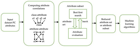
Figure 5. Phases of correlation-based feature selection method.

Best First with Forward search direction is one of the most extensively used search methods in the CFS attribute evaluation. Forward search begins with an empty feature set and gradually adds features in subsequent cycles. A stop criterion is implemented to prevent the best first search from searching the whole attribute subset search area. If five consecutive fully extended subsets demonstrate no enhancement over the present best subset, the search will be terminated. The dataset is made up of PC attributes that are supplied to the CFS function. CFS computes class-attribute and attribute-attribute correlations before searching the attribute subset space. The subset selected during the search with the highest merit (as determined by Equation (1)) is utilized to reduce the dimensionality of the original data. After that, the reduced dataset can be fed into a machine learning algorithm for training and validation.

By performing the processes as illustrated in Figure 5, the CFS method evaluated a total of 98 subsets. With the best subset merit value of 0.335, the CFS method selected six transformed components out of 18, which accounted for just 33.33% of the entire feature dimension. The optimal components 1, 3, 6, 8, 13, and 16 were included from Table 2 to assess the machine learning model’s performance.

3.6. Machine Learning Classifiers

In this work, three single classifiers, Support Vector Machines, K-Nearest Neighbors, and J48 Decision Tree, and three ensemble classifiers AdaBoost M1, Bagging, and Rotation Forest were employed to predict the accuracy of coronary heart disease risk. The brief discussion about the classifiers is as follows.

3.6.1. Support Vector Machines

Support Vector Machines is a supervised machine learning algorithm to solve classification issues based on the theory of statistics [52]. For a given training dataset of n points, $\left(x_1,y_1\right)\left(x_2,y_2\right),\dots \left(x_n,y_n\right)$, where $y_i$ is 1 or −1, representing the class to which the point, $x_i$ belongs to. A hyperplane is defined as a set of data points x that satisfy the equation

$$w^{\mathrm{T}}.x-b=0$$

(2)

where $w$ is a normal vector, perpendicular to the hyperplane’s surface, and b is the value of the offset from the origin. The $\frac{b}{\parallel w\parallel }$ parameter defines the hyperplane’s offset from the origin along the normal vector $w$.

Kernel or Kernel trick is the process of utilizing a linear classifier to resolve nonlinear problems. The commonly used SVM kernels are Polynomial, Radial Basis Function (RBF), and Pearson VII Universal Kernel (PUK).

The Polynomial kernel for the degree d is defined as

$$K\left(x,y\right)={\left(x^{T}y+c\right)}^d$$

(3)

where x and y are the feature vectors of input space, and c is a constant. The second most widely used kernel is RBF, defined as

$$K\left(x, x^{\prime }\right)=\exp \left(-\frac{{\parallel x-x^{\prime }\parallel }^2}{2{\sigma }^2}\right)$$

(4)

where $x$ and $x^{\prime }$ are the feature vectors of input space, $\sigma$ is a constant. The Pearson VII function of PUK is defined as

$$f\left(x\right)=\frac{H}{{\left. [1+{\left(\frac{2\left(x-x_0\right)\sqrt{2^{\frac{1}{\omega }}-1}}{\sigma }\right)}^2\right]}^{\omega }}$$

(5)

where the $H$ is the peak height at $x_0$, $x$ is an independent variable, and the parameters $\omega$, and $\sigma$ control the width and tailing factor of the peak [53].

3.6.2. K-Nearest Neighbors

The K-Nearest Neighbors algorithm determines the class of an instance by comparing it to a nearby instance from the training dataset [12]. The distance measure is utilized to calculate the neighbors, which can be chosen from a variety of possibilities. Euclidean distance is the most widely used distance metric for numeric variables [51]. Giving each neighbor a weight of 1/d, where d is the distance between them, is a popular weighing approach [54]. The parameter to be optimized for the KNN classifier are the number of nearest neighbors and the distance weighting.

3.6.3. Decision Tree

The representation of the decision tree model is a binary tree. Each internal node in a classification tree is labeled with an input attribute, and the node’s output leads to a subordinate decision node on a different input attribute. A target class variable is labeled on each leaf of the tree [55]. Each node represents a split point on a single input variable (x) (assuming the variable is numeric). The tree’s leaf nodes have an output variable (y) that is used to create a prediction. Predictions are created by going through the tree’s splits until reaching a leaf node and then displaying the class value at that node [56]. For the J48 decision tree, the important parameters to be tuned are the confidence factor and the minimum number of instances for the leaf.

3.6.4. AdaBoost M1

The most ideal method to operate with AdaBoost M1 is the decision tree with one classification decision, known as the decision stump [57]. The training data are used to build a weak classifier that is a decision stump using the weighted observations. Each decision stump makes a single decision on one input parameter and returns a first- or second-class result of +1.0 or −1.0 because only binary classification problems are allowed. Weak classifiers are introduced one by one and trained using weighted training data [58]. For every sample in the training dataset, each weak learner provides an output hypothesis h() that fixes a prediction $h\left(x_i\right)$. A weak learner is chosen and given a coefficient, ${\alpha }_t$, at each iteration t so that the total training error, $E_t$, given in (6) of the resultant t-stage boosting classifier is minimized.

$$E_t={\displaystyle \sum }_{i}E\left. [F_{t-1}\left(x_i\right)+{\alpha }_{t}h\left(x_i\right)\right]$$

(6)

where $F_{t-1}\left(x\right)$ is the boosted classifier that was created during the earlier training stage, $E\left(F\right)$ is the error function, and ${\alpha }_{t}h\left(x_i\right)=f_t\left(x\right)$ is the weak classifier under consideration for inclusion in the final classifier [59]. The parameters of the AdaBoostM1 algorithm to be optimized are the base classifier and the number of iterations.

3.6.5. Bagging

Bagging generates m new training sets, $D_i$ named as the bootstrap sample, each of size $n^{\prime }$, by sampling original training dataset D of size n uniformly with replacement. Some samples may be replicated in each $D_i$ by sampling with replacement. If, $n^{\prime }=n$, then the set $D_i$ is anticipated to include the percentage (1 − 1/e) (63.2%) of the unique samples of D, with the remainder being duplicated, for big n [60]. Then, using these m bootstrap samples, m models are trained and integrated by averaging the outcome (for regression) or polling (for classification). Thereafter, the ensemble generates decision trees from bootstrapping samples, by assessing each feature and calculating the number of samples for which the feature’s existence or absence results in a positive or negative outcome [61]. The reduced error pruning tree (REPTree) is used as the default base classifier of the Bagging. The parameters of Bagging to be optimized are the base classifier and the number of iterations.

3.6.6. Rotation Forest

The Rotation Forest partitions the feature set for each tree and performs a principal component analysis on each feature subset before recombining the retrieved features over the whole training set [62]. It performs sampling independently on each feature subset for each tree. Steps involved in constructing a rotation forest algorithm are as follows:

Let T be the number of trees needed to be developed. For each tree T:

Split the features of the training dataset into K disjoint subsets randomly of equal size. Each feature subset consists of M = n/K features. For each of the K datasets:

Bootstrap 75 percent of the data from each K dataset and use the bootstrapped sample in subsequent phases.

On the i-th subset in K, perform a principal component analysis. All the principal components should be kept to preserve the variability of information in the dataset. Every feature j in the K-th subset will have a principal component, a. Let a_ij be the principal component for the i-th subset’s j-th attribute.

Store all the principal components for each subset.

Make an $n\times \sum _j{M}_j$ rotation matrix $R_i$, with n equaling the total number of features. Rearrange the principal components in the matrix such that they correspond to the feature’s position in the original training dataset X.

$$R_i=\left. [\begin{array}{c}\begin{array}{cccc}{a}_{i1}^{\left(1\right)},\dots ,a_{i1}^{\left(M_1\right)}& \left. [0\right]& \cdots & \left. [0\right]\\ \left. [0\right]& a_{i2}^{\left(1\right)}, \dots ,a_{i2}^{\left(M_2\right)}& \cdots & \left. [0\right]\\ ⋮& ⋮& \ddots & ⋮\\ \left. [0\right]& \left. [0\right]& \cdots & a_{iK}^{\left(1\right)}, \dots ,a_{iK}^{\left(M_K\right)}\end{array}\end{array}\right]$$

(7)

Using matrix multiplication, project the training dataset onto the rearranged rotation matrix, $R_i^a$, and create a decision tree with the projected dataset. Save the tree as well as the rotation matrix to compute the confidence of the input instance [63].

The base classifier used, the number of iterations to be performed, and the percentage of instances to be removed were optimized in the Rotation Forest ensemble.

3.7. Hyperparameter Optimization

Hyperparameters are crucial for machine learning algorithms because they directly regulate the behavior of training algorithms and have a major impact on model performance. Although many hyperparameters have known characteristics, it is unknown what impact they will impose on the performance of the final model on a particular dataset [64]. Hence, the adoption of the type of hyperparameters and tuning technique has a direct bearing on the enhancement of its efficiency. Consequently, the goal of optimization is to minimize the cost function or total error while optimizing the performance measure of the machine learning algorithm on training data. The hyperparameters and their value range of machine learning modes tuned in this work are listed in Table 5.

Table 5. Hyperparameters and their value range of machine learning models.

Classifier	Hyperparameters	Value Range
SVM	Complexity parameter, C	1–7
	Type of kernel	PolyKernel, PUK, RBF
KNN	Number of neighbors, K	1, 3, 5, 7
	Distance weighting	No distance weighting, 1/distance, 1-distance
J48	Confidence factor, C	0.25, 0.50, 0.75
	Minimum number of instances per leaf, M	1–3
AdaBoostM1	Base classifier	Decision stump, J48
	Number of iterations, I	10, 20, 30
Bagging	Base classifier	REPTree, J48
	Number of iterations, I	10, 20, 30
ROTF	Base classifier	J48, Random Forest
	Number of iterations, I	10, 20, 30
	Removed percentage, P	40, 50

From Table 5, the typical hyperparameters that show the impact on the model’s performance in improving the prediction risk of coronary heart disease have been included in this work.

3.8. Performance Metrics

The confusion matrix shown in Table 6 depicts the evaluation of various performance metrics of a classifier. True positives are the number of responses proportional to the positive class that were correctly predicted as positive. True negatives are the number of responses equal to the negative class that were correctly predicted as negative. False positives are the number of responses equivalent to the negative class but predicted as positive. False negatives are the number of responses equal to the positive class but predicted as negative.

Table 6. Confusion Matrix.

	Predicted Class
		Low Risk (0)	High Risk (1)
True class	Low risk (0)	True Negative (TN)	False Positive (FP)
	High risk (1)	False Negative (FN)	True Positive (TP)

The performance metrics such as accuracy, sensitivity (recall), specificity, precision, F-measure, the area under the ROC curve, cost, and training time of the machine learning models are computed using the confusion matrix in Table 6.

4. Results and Analysis

The results of machine learning classifiers on the complete set of principal components and optimal components selected from the CFS method, followed by the results of hyperparameter optimization on the optimal set of principal components and comparative analysis with the related works, are discussed in this section.

4.1. Results of Classifiers without Hyperparameter Optimization

The performance metrics of the machine learning classifiers with 10-fold cross-validation on the complete set of 18 principal components (PCs) and six optimal PCs selected from CFS with the Best First search method are provided in Table 7.

Table 7. Performance comparison of machine learning algorithms on a complete and optimal set of principal components.

	On a Complete Set of PCs								On Optimal PCs
Model	Acc.	Sen.	Spe.	Pre.	F-mea.	AUC	Cost	Time (ms)	Acc.	Sen.	Spe.	Pre.	F-mea.	AUC	Cost	Time (ms)
SVM	84.82	84.82	83.62	85.00	84.91	0.842	87	100	84.64	84.64	83.00	85.14	84.89	0.838	88	50
KNN	96.34	96.34	96.10	96.34	96.34	0.945	21	0	95.81	95.81	95.73	95.81	95.81	0.963	24	0
J48	92.32	92.32	92.38	92.36	92.34	0.965	44	120	93.89	93.89	93.68	93.89	93.89	0.967	35	10
AB	81.85	81.85	80.30	82.15	82.00	0.913	104	150	87.26	87.26	86.45	87.32	87.29	0.953	73	30
BG	89.35	89.35	88.51	89.46	89.41	0.967	61	160	91.97	91.97	91.69	91.97	91.97	0.970	46	40
RTF	96.16	96.16	96.02	96.16	96.16	0.996	22	800	95.99	95.99	95.40	96.09	96.04	0.992	23	120

Acc.—Accuracy, Sen.—Sensitivity, Spe.—Specificity, F-mea.—F-measure, AUC—Area Under the ROC curve, ms—milliseconds.

Table 7 shows that, on a complete set of PCs, the KNN classifier produced the best accuracy of 96.34% at a cost of 21 instances in 0 ms while the RTF classifier delivered an accuracy of 96.16% and the highest AUC of 0.996 at a cost of 22 observations in 800 ms. In comparison, on optimal PCs, the accuracy of J48, AB, and BG classifiers has been improved while that of SVM, KNN, and RTF classifiers has been decreased. RTF attained the best accuracy of 95.99% and an AUC of 0.992 at a cost of 23 samples in 120 ms. The accuracy of KNN has dropped to 95.81%, and its AUC increased to 0.963 in 0 ms. The other metrics such as sensitivity, specificity, precision, and F-measure are equivalent to the accuracy value since they have been computed as the weighted average of both target class 0 and 1. The ROC plots of the Rotation Forest ensemble on complete and optimal components are shown in Figure 6.

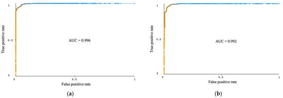
Figure 6. ROC plots of the Rotation Forest ensemble classifier with J48 as the base classifier. (a) Using a complete set of principal components; (b) using optimal set of principal components.

Figure 6a shows the ROC plot, that is, the true positive rate versus the false positive rate of the Rotation Forest ensemble with the J48 base classifier on 18 principal components of the combined dataset with an AUC of 0.996. Figure 6b shows the ROC plots of the Rotation Forest on six optimal components selected from the CFS method with an AUC of 0.992. Overall, with the dimensionality reduction, the accuracy of SVM, KNN, and RTF has declined, and that of J48, AB, and BG has increased, the AUC of all the classifiers has improved except for SVM, and the training time of all the classifiers has dropped to more than 50%. The KNN classifier stood as the best algorithm on full PCs with the cost of just 21 instances out of 573 in 0 ms of training time. The comparison of the model’s training time is shown in Figure 7.

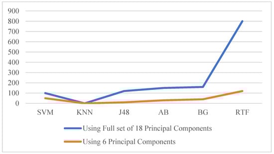
Figure 7. Comparison of the model’s training time (in milliseconds).

Figure 7 shows that the training time of the models on an optimal set of principal components by removing the irrelevant ones using the CFS method has significantly dropped, especially for the Rotation Forest ensemble, compared to that on a complete set of components.

4.2. Results of Classifiers with Hyperparameter Optimization

Our proposed work mainly aims to determine the best predictive model for coronary heart disease risk by comparing the performance of the various supervised machine learning models. However, the optimum performance of the model can be achieved by configuring the best parameters during the modeling process. Therefore, we performed the hyperparameter optimization to find the best hyperparameters of the classifier at which it will provide the best predictive outcomes on the selected components. In order to assess the performance of the classifier, a batch size of 100 instances was utilized for all the experiments.

4.2.1. Hyperparameter Optimization of SVM

For the SVM classifier, the complexity parameter (C) and the Kernel function were adjusted in this work. The complexity parameter (C) in SVM determines how often the classifier avoids making mistakes when classifying the training instances. The results of SVM hypermeter optimization are provided in Table 8.

Table 8. Prediction accuracy of support vector machine hyperparameter optimization.

Training No.	Complexity Parameter, C	Kernel	Accuracy
1.	1	PolyKernel	84.6422
2.	2	PolyKernel	84.8168
3.	3	PolyKernel	84.6422
4.	4	PolyKernel	84.8168
5.	5	PolyKernel	84.9913
6.	6	PolyKernel	84.9913
7.	7	PolyKernel	84.8168
8.	1	Pearson VII Universal	87.2600
9.	2	Pearson VII Universal	89.8778
10.	3	Pearson VII Universal	90.4014
11.	4	Pearson VII Universal	91.2740
12.	5	Pearson VII Universal	91.7976
13.	6	Pearson VII Universal	92.6702
14.	7	Pearson VII Universal	93.1937
15.	1	Radial Basis Function	69.6335
16.	2	Radial Basis Function	85.3403
17.	3	Radial Basis Function	84.2932
18.	4	Radial Basis Function	83.7696
19.	5	Radial Basis Function	84.2932
20.	6	Radial Basis Function	83.7696
21.	7	Radial Basis Function	83.7696

From Table 8, a total of 21 trainings were performed by changing the C values from 1 to 7, and three kernels, namely PolyKernel, Pearson VII Universal Kernel (PUK) function, and Radial Basis Function (RBF), were used. The SVM with PUK and C = 7 produced the best accuracy of 93.1937% at the 14th training, which accounted for an 8.55% improvement.

4.2.2. Hyperparameter Optimization of KNN

For the KNN classifier, the distance function for finding the neighbors is maintained as Euclidean distance for all the trainings. The number of nearest neighbors (K) and the distance weighting (no distance weighting, weight by 1/distance, weight by 1-distance) were tuned, and the results are provided in Table 9.

Table 9. Prediction accuracy of k-nearest neighbor hyperparameter optimization.

Training No.	Number of Neighbors, K	Distance Weighting	Accuracy
1.	1	No distance weighting	95.8115
2.	3	No distance weighting	89.5288
3.	5	No distance weighting	85.1658
4.	7	No distance weighting	84.8168
5.	1	1/distance	95.8115
6.	3	1/distance	96.6841
7.	5	1/distance	97.0332
8.	7	1/distance	96.6841
9.	1	1-distance	95.8115
10.	3	1-distance	90.4014
11.	5	1-distance	88.3072
12.	7	1-distance	85.3403

From Table 9, a total of 12 experiments were conducted by changing the K values such as 1, 3, 5, and 7 for each distance weighting function. For K = 1, the classifier yielded the same accuracy of 95.8115% on various distance functions. As the K value increased, the accuracy was decreased with no distance and 1-distance weighting functions. The best prediction accuracy of 97.0332% has obtained at K = 5, with an inverse distance weighting function at the 7th training.

4.2.3. Hyperparameter Optimization of J48 DT

For the J48 decision tree classifier, the confidence factor (C) used for pruning and the minimum number of instances per leaf (M) were tuned with the unpruned option as False for all the trainings. The results are provided in Table 10.

Table 10. Prediction accuracy of j48 decision tree hyperparameter optimization.

Training No.	Confidence Factor, C	Min. Number of Instances per Leaf, M	Accuracy
1.	0.25	1	95.1134
2.	0.25	2	93.8918
3.	0.25	3	93.1937
4.	0.50	1	95.1134
5.	0.50	2	93.8918
6.	0.50	3	93.5428
7.	0.75	1	95.4625
8.	0.75	2	93.8918
9.	0.75	3	92.6702

From Table 10, J48 has been trained 9 times by changing the C values to 0.25, 0.5, and 0.75 and M values to 1, 2, and 3. The accuracy of J48 at M = 1, C = 0.25 and 0.5 is 95.1134%, and the accuracy at M = 2, C = 0.25, 0.5 and 0.75 is 93.8918%. The best accuracy yielded by J48 is 95.4625% at an M value of 1 and a C value of 0.75 at the 7th training.

4.2.4. Hyperparameter Optimization of AdaBoost M1

For the AdaBoost M1 ensemble, the base classifier and the number of iterations (I) to be performed were tuned to improve its performance in predicting heart disease. The weight threshold has been maintained at 100 for all the trainings. The results of AdaBoost M1 hyperparameter optimization are given in Table 11.

Table 11. Prediction accuracy of Adaboost M1 hyperparameter optimization.

Training No.	Base Classifier	Number of Iterations, I	Accuracy
1.	Decision Stump	10	87.2600
2.	Decision Stump	20	90.0524
3.	Decision Stump	30	90.9250
4.	J48	10	97.2077
5.	J48	20	97.0332
6.	J48	30	97.3822

From Table 11, the AdaBoost M1 has been trained 6 times by changing the base classifier Decision Stump and J48 with the number of iterations values as 10, 20, and 30 for each case. With this optimization, it provided remarkable performance improvement, about a 10% of increase in accuracy. The best accuracy of 97.3822% has been achieved using J48 as the base classifier and I = 30 at the 6th training.

4.2.5. Hyperparameter Optimization of Bagging

For the bagging, the base classifier and the number of iterations were tuned, and the results are shown in Table 12.

Table 12. Prediction accuracy of bagging hyperparameter optimization.

Training No.	Base Classifier	Number of Iterations, I	Accuracy
1.	REPTree	10	91.9721
2.	REPTree	20	91.6230
3.	REPTree	30	92.6702
4.	J48	10	94.2408
5.	J48	20	94.7644
6.	J48	30	94.4154

From Table 12, the bagging yielded the best accuracy of 94.7644% using J48 as the base classifier and I = 20 at the 5th training. For both AdaBoost and Bagging, the base classifier J48 maintains the values of C = 0.25 and M = 2.

4.2.6. Hyperparameter Optimization of RTF

For the Rotation Forest ensemble, along with the base classifier and number of iterations, the percentage of instances to be removed (P) is also tuned. The results of Rotation Forest hyperparameter optimization are postulated in Table 13.

Table 13. Prediction accuracy of rotation forest hyperparameter optimization.

Training No.	Base Classifier	Number of Iterations, I	Removed Percentage, P	Accuracy
1.	J48	10	50	95.9860
2.	J48	20	50	95.9860
3.	J48	30	50	96.3351
4.	J48	10	40	95.2880
5.	J48	20	40	95.9860
6.	J48	30	40	95.9860
7.	RF	10	50	97.7312
8.	RF	20	50	97.5567
9.	RF	30	50	97.7312
10.	RF	10	40	97.9058
11.	RF	20	40	97.7312
12.	RF	30	40	97.7312

From Table 13, Rotation Forest has been trained 12 times by tuning the base classifiers (J48 and Random Forest), iterations (10, 20, and 30), and removed percentage (50 and 40). The base classifier Random Forest provided a betterment in accuracy by about 2% compared to that offered by J48. The utmost accuracy of 97.9058% is attained at I = 10 and P = 40 at the 10th training.

The accuracy comparison of machine learning models without and with optimization on selected principal components from the CFS method is provided in Table 14.

Table 14. Accuracy comparison of machine learning models without and with optimization.

No.	Classifier	Without Optimization	With Optimization	Improvement
1.	Support Vector Machines	84.64	93.19	8.55
2.	K-Nearest Neighbors	95.81	97.03	1.22
3.	J48 Decision Tree	93.89	95.46	1.57
4.	AdaBoost M1	87.26	97.38	10.12
5.	Bagging	91.97	94.76	2.79
6.	Rotation Forest	95.99	97.91	1.92

From Table 14, the accuracy of machine learning models without optimization varied between 84% and 96%, while with optimization, the accuracy varied between 93% and 98%. The variation in accuracy has dropped from about 12% to 5% with optimization. The bar plot of the accuracy comparison with and without optimization is shown in Figure 8.

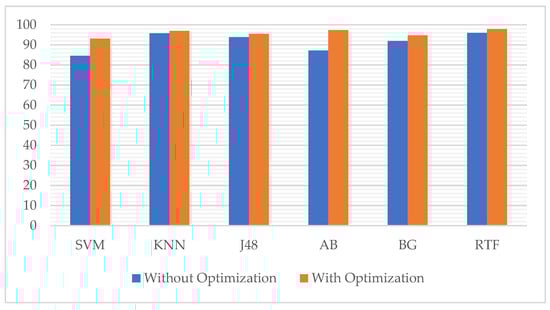
Figure 8. Accuracy comparison of machine learning models without and with optimization.

It is observed from Figure 8 that hyperparameter optimization has improved the accuracy of all models. The most remarkable improvement has been achieved by AdaBoost M1 with 10%, followed by SVM with 8.55%. The KNN model was the least improved, with an increase of 1.22%. The J48 accuracy has increased by about 1.57%. The accuracy of Bagging and Rotation Forest ensembles has been enhanced by about 2.79% and 1.92%, respectively. The maximum performance measures of the classifiers after hyperparameter optimization are provided in Table 15.

Table 15. Maximum performance measures of the classifiers after hyperparameter optimization.

On Selected Six Principal Components by the CFS Method
Model	Acc.	Sen.	Spe.	Pre.	F-mea.	AUC	Cost	Best Hyperparameters
SVM	93.19	93.19	92.56	93.28	93.24	0.929	39	C = 7, PUK kernel
KNN	97.03	97.03	96.88	97.04	97.03	0.988	17	K = 5, 1/distance weight
J48	95.46	95.46	95.24	95.5	95.46	0.969	26	C = 0.75, M = 1
AB	97.38	97.38	97.10	97.40	97.39	0.989	15	J48 base classifier, I = 30
BG	94.76	94.76	94.46	94.77	94.77	0.987	30	J48 base classifier, I = 20
RTF	97.91	97.91	97.66	97.92	97.91	0.996	12	RF base classifier, I = 10, P = 40

From Table 15, the Rotation Forest ensemble outperformed other classifiers with an accuracy of 97.91%, sensitivity of 97.91%, specificity of 97.66%, precision of 97.92%, F-measure of 97.91%, and AUC of 0.996 using the Random Forest as the base classifier. The total number of misclassified instances has been reduced to 12 out of 573 instances. The classifier errors plot of the Rotation Forest is shown in Figure 9.

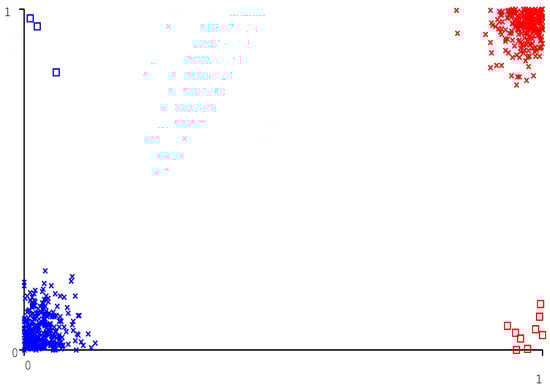
Figure 9. Classifier errors plot of rotation forest ensemble.

From Figure 9, the squares indicate incorrectly classified instances, and the cross marks denote correctly classified instances. The three blue squares indicate that three instances are incorrectly predicted as the presence of heart disease, and the nine red squares signify the nine instances are incorrectly predicted as the absence of heart disease. The blue cross marks indicate the instances that are correctly classified as the absence of heart disease, and the red cross marks imply the instances that are correctly classified as the presence of heart disease. The ROC plot of the Rotation Forest ensemble after optimization is shown in Figure 10.

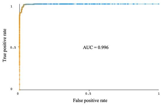
Figure 10. Roc plot of the rotation forest ensemble after optimization.

From Figure 10, the area under the ROC curve of the Rotation Forest ensemble on optimal components is 0.996, the same as that obtained with this ensemble on the complete set of principal components as in Figure 6a. An AUC value close to 1 indicates that the model can achieve a high true positive rate, the proportion of instances that are correctly identified as positive for the disease, while still maintaining a low false-positive rate, the proportion of individuals who are incorrectly classified as positive for the disease. The bar chart of the machine learning model’s cost (incorrectly classified instances) utilizing optimal components, based on Table 7 and Table 15, without and with hyperparameter optimization, is shown in Figure 11.

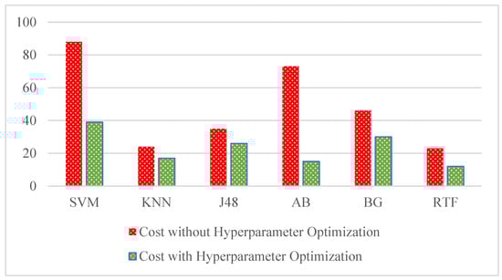
Figure 11. Cost comparison of machine learning models without and with optimization.

From Figure 11, the cost of all machine learning models has decreased with hyperparameter optimization. Specifically, the AdaBoost M1 model achieved a remarkable drop in cost from 73 to 15 instances, followed by the SVM classifier from 88 to 39 instances. The best-performed ensemble Rotation Forest has yielded a reduction in cost from 23 to 12 instances.

5. Discussion

The performance comparison of the proposed work with the state-of-the-art works in coronary heart disease risk prediction is provided in Table 16.

Table 16. Performance comparison of related works.

No.	Ref.	Year	FS	Classifier	#	Acc.	Sen.	Spe.	Pre.	F-mea.	AUC
1.	[31]	2019	RSA	RF	7	93.33	95.12	89.79	-	-	0.947
2.	[32]	2019	Relief	RF	12	85.50	85.60	-	85.50	85.50	0.915
3.	[33]	2020	PPA	KNN	4	86.17	-	85.00	-	-	-
4.	[34]	2020	NFR	LR	9	92.53	-	-	-	-	0.926
5.	[35]	2019	FFSA	SVM RBF	7	81.19	72.92	88.68	-	-	-
6.	[36]	2021	LASSO	DL	6	94.20	83.10	82.30	-	-	-
7.	[37]	2020	Relief	Extra Tree	6	94.41	94.93	94.89	95.46	95.00	0.942
8.	[38]	2019	Chi-square	DL	11	93.33	85.36	100	-	-	0.94
9.	[39]	2022	Pearson’s correlation	CatBoost	10	94.34	-	-	-	-	-
10.	[40]	2022	-	LR	13	92.30	96.08	87.50	90.74	93.34	-
11.	[41]	2022	-	SVM	13	96.72	98.00	-	98.00	98.00	-
12.	[42]	2022	Correlation	RF	-	83.00	-	-	-	-	-
13.	[45]	2020	RTs	RTs	44	91.47	-	-	-	-	0.967
14.	[46]	2020	Tree-based	BiGRU +CNN	60	96.00	92.00	-	99.00	95.00	0.990
15.	Proposed work	2022	PCA + CFS	Rotation Forest	6	97.91	97.91	97.66	97.92	97.91	0.996

FS—Feature Selection method, #—No. of features, RSA—Random Search Algorithm, RF—Random Forest, PPA—Parasitic-Predation Algorithms, NFR—Novel Feature Reduction, FFSA—Forward Feature Selection Algorithm, LASSO—Least Absolute Shrinkage and Selection Operator, DL—Deep Learning.

From Table 16, although prior studies employed feature selection and ensemble techniques, the highest accuracy obtained was 94.41% by Muhammad et al. [37] with the use of 6 optimal features (age, cp, fbs, ca, thal, and thalach) of the Cleveland dataset obtained from the Relief feature selection method and Extra Tree classifier. Bharti et al. [36] attained 94.20% with the six features (age, sex, exang, oldpeak, ca, and trestbps) obtained from the LASSO FS technique and Deep Learning. Ali et al. [38] achieved 100% specificity on the test set of 90 samples, but the accuracy (93.33%) is about 7% less, and the sensitivity (85.36%) is about 15% less than the specificity achieved. Javeed et al. [31] and Muhammad et al. [37] attained an AUC value of 0.947 and 0.942, respectively. Saboor et al. [41] achieved the utmost accuracy of 96.72% by standardization and tuning the hyperparameters of the SVM model on the full features of the Cleveland dataset. Joloudari et al. [45] used the random trees to rank the features of Al-Zadeh Sani’s heart data and achieved 91.47% of accuracy with the 44 selected features. The ensemble of deep learning networks employed in [46] selected 60 features from a tree-based random classifier and achieved 99% of precision but the accuracy is 3% less than that. In this work, eighteen (18) principal components have been obtained by specifying parameters variance covered as 0.95 and maximum attributes names as 5. Then, CFS with the best first search method was applied to select the best components to reduce the training time and we utilized 10-fold cross-validation for evaluating the performance of the machine learning classifiers. Cross-validation is a statistical resampling approach that tests and trains a machine learning model using various parts of the data on successive iterations. It also mitigates the risk of overfitting. Further, hyperparameter tuning of classifiers has been carried out to improve the predictive performance of the classifiers. Overall, our proposed work outperformed the related works with 97.91% of accuracy by employing six optimal principal components selected from the CFS method and optimizing the parameters of the Rotation Forest ensemble with the Random Forest as the base classifier. Our work provided about 4.6% higher accuracy than that in [38].

6. Conclusions and Future Work

The performance of machine learning models in predicting coronary heart disease risk has been improved by applying correlation-based feature selection to choose the best set of principal components from the combined (Cleveland + Statlog) heart dataset, and hyperparameter optimization to find the best hyperparameters for the models (SVM, KNN, J48 DT, AdaBoost M1, Bagging, and Rotation Forest) detailed in this paper. It has been shown that the training time of the classifiers has decreased when the feature selection is employed to eliminate the irrelevant components. In contrast, the classifier’s performance has improved with the hyperparameter optimization by reducing the number of incorrectly classified instances. The Rotation Forest ensemble with Random Forest as the base classifier achieved the utmost accuracy of 97.91% and AUC of 0.996 at the cost of 12 out of 573 instances using six principal components selected from the CFS method. The AdaBoost M1 with J48 as the base classifier yielded the highest improvement in accuracy about 10% followed by the SVM of 8.55%. The KNN classifier is trained in 0 ms of time on a full and optimal set of components. The hyperparameter optimization increased the training time of the machine learning models on the selected components because the tuning process has been carried out manually. In future, automatic hyperparameter optimization and new feature selection techniques could be considered to further improve the predictive performance of the machine learning models.

References

- Ghiasi, M.M.; Zendehboudi, S.; Mohsenipour, A.A. Decision tree-based diagnosis of coronary artery disease: CART model. Comput. Methods Programs Biomed. 2020, 192, 105400. [Google Scholar] [CrossRef] [PubMed]
- Fitriyani, N.L.; Syafrudin, M.; Alfian, G.; Rhee, J. HDPM: An Effective Heart Disease Prediction Model for a Clinical Decision Support System. IEEE Access 2020, 8, 133034–133050. [Google Scholar] [CrossRef]
- Yadav, D.C.; Pal, S. Prediction of Heart Disease Using Feature Selection and Random Forest Ensemble Method. Int. J. Pharm. Res. 2020, 12, 56–66. [Google Scholar] [CrossRef]
- Shahid, A.H.; Singh, M.P.; Roy, B.; Aadarsh, A. Coronary Artery Disease Diagnosis Using Feature Selection Based Hybrid Extreme Learning Machine. In Proceedings of the 2020 3rd International Conference on Information and Computer Technologies (ICICT), San Jose, CA, USA, 9–12 March 2020; pp. 341–346. [Google Scholar] [CrossRef]
- WHO. 2020. [Online]. Available online: https://www.who.int/health-topics/cardiovascular-diseases/#tab=tab_1 (accessed on 14 October 2021).
- Ryu, H.; Moon, J.; Jung, J. Sex Differences in Cardiovascular Disease Risk by Socioeconomic Status (SES) of Workers Using National Health Information Database. Int. J. Environ. Res. Public Health 2020, 17, 2047. [Google Scholar] [CrossRef] [PubMed]
- Yang, H.; Garibaldi, J.M. A hybrid model for automatic identification of risk factors for heart disease. J. Biomed. Inform. 2015, 58, S171–S182. [Google Scholar] [CrossRef] [PubMed]
- Sowmiya, C.; Sumitra, P. Analytical study of heart disease diagnosis using classification techniques. In Proceedings of the 2017 IEEE International Conference on Intelligent Techniques in Control, Optimization and Signal Processing (INCOS), Srivilliputtur, India, 23–25 March 2017; pp. 1–5. [Google Scholar] [CrossRef]
- Karthick, D.; Priyadharshini, B. Predicting the chances of occurrence of Cardio Vascular Disease (CVD) in people using classification techniques within fifty years of age. In Proceedings of the 2018 2nd International Conference on Inventive Systems and Control (ICISC), Coimbatore, India, 19–20 January 2018; pp. 1182–1186. [Google Scholar] [CrossRef]
- Dinesh, K.G.; Arumugaraj, K.; Santhosh, K.D.; Mareeswari, V. Prediction of Cardiovascular Disease Using Machine Learning Algorithms. In Proceedings of the 2018 International Conference on Current Trends towards Converging Technologies (ICCTCT), Coimbatore, India, 1–3 March 2018; pp. 1–7. [Google Scholar] [CrossRef]
- Gupta, A.; Kumar, R.; Arora, H.S.; Raman, B. MIFH: A Machine Intelligence Framework for Heart Disease Diagnosis. IEEE Access 2019, 8, 14659–14674. [Google Scholar] [CrossRef]
- Louridi, N.; Amar, M.; El Ouahidi, B. Identification of Cardiovascular Diseases Using Machine Learning. In Proceedings of the 2019 7th Mediterranean Congress of Telecommunications (CMT), Fez, Morocco, 24–25 October 2019; pp. 1–6. [Google Scholar] [CrossRef]
- Javeed, A.; Rizvi, S.S.; Zhou, S.; Riaz, R.; Khan, S.U.; Kwon, S.J. Heart Risk Failure Prediction Using a Novel Feature Selection Method for Feature Refinement and Neural Network for Classification. Mob. Inf. Syst. 2020, 2020, 8843115. [Google Scholar] [CrossRef]
- Vasant, P.; Ganesan, T.; Elamvazuthi, I.; Webb, J.F. Interactive fuzzy programming for the production planning: The case of textile firm. Int. Rev. Model. Simul. 2011, 4, 961–970. [Google Scholar]
- Ali, Z.; Alsulaiman, M.; Muhammad, G.; Elamvazuthi, I.; Mesallam, T.A. Vocal fold disorder detection based on continuous speech by using MFCC and GMM. In Proceedings of the 2013 7th IEEE GCC Conference and Exhibition (GCC), Doha, Qatar, 17–20 November 2013; pp. 292–297. [Google Scholar] [CrossRef]
- Gupta, R.; Elamvazuthi, I.; Dass, S.C.; Faye, I.; Vasant, P.; George, J.; Izza, F. Curvelet based automatic segmentation of supraspinatus tendon from ultrasound image: A focused assistive diagnostic method. Biomed. Eng. Online 2014, 13, 157. [Google Scholar] [CrossRef]
- Ali, Z.; Alsulaiman, M.; Elamvazuthi, I.; Muhammad, G.; Mesallam, T.A.; Farahat, M.; Malki, K.H. Voice pathology detection based on the modified voice contour and SVM. Biol. Inspired Cogn. Arch. 2016, 15, 10–18. [Google Scholar] [CrossRef]
- Ali, Z.; Elamvazuthi, I.; Alsulaiman, M.; Muhammad, G. Detection of Voice Pathology using Fractal Dimension in a Multiresolution Analysis of Normal and Disordered Speech Signals. J. Med. Syst. 2016, 40, 20. [Google Scholar] [CrossRef] [PubMed]
- Nurhanim, K.; Elamvazuthi, I.; Izhar, L.; Capi, G.; Su, S. EMG Signals Classification on Human Activity Recognition using Machine Learning Algorithm. In Proceedings of the 2021 8th NAFOSTED Conference on Information and Computer Science (NICS), Hanoi, Vietnam, 21–22 December 2021; pp. 369–373. [Google Scholar] [CrossRef]
- Rahim, K.N.K.A.; Elamvazuthi, I.; Izhar, L.I.; Capi, G. Classification of Human Daily Activities Using Ensemble Methods Based on Smartphone Inertial Sensors. Sensors 2018, 18, 4132. [Google Scholar] [CrossRef] [PubMed]
- Sharon, H.; Elamvazuthi, I.; Lu, C.-K.; Parasuraman, S.; Natarajan, E. Development of Rheumatoid Arthritis Classification from Electronic Image Sensor Using Ensemble Method. Sensors 2019, 20, 167. [Google Scholar] [CrossRef] [PubMed]
- Reddy, K.V.V.; Elamvazuthi, I.; Aziz, A.A.; Paramasivam, S.; Na Chua, H.; Pranavanand, S. Rotation Forest Ensemble Classifier to Improve the Cardiovascular Disease Risk Prediction Accuracy. In Proceedings of the 2021 8th NAFOSTED Conference on Information and Computer Science (NICS), Hanoi, Vietnam, 21–22 December 2021; pp. 404–409. [Google Scholar] [CrossRef]
- Reddy, K.V.V.; Elamvazuthi, I.; Aziz, A.A.; Paramasivam, S.; Na Chua, H.; Pranavanand, S. Heart Disease Risk Prediction Using Machine Learning Classifiers with Attribute Evaluators. Appl. Sci. 2021, 11, 8352. [Google Scholar] [CrossRef]
- Maurovich-Horvat, P. Current trends in the use of machine learning for diagnostics and/or risk stratification in cardiovascular disease. Cardiovasc. Res. 2021, 117, e67–e69. [Google Scholar] [CrossRef]
- Gonsalves, A.H.; Thabtah, F.; Mohammad, R.M.A.; Singh, G. Prediction of Coronary Heart Disease using Machine Learning. In Proceedings of the 2019 3rd International Conference on Deep Learning Technologies, Xiamen China, 5–7 July 2019; pp. 51–56. [Google Scholar] [CrossRef]
- Uddin, S.; Khan, A.; Hossain, E.; Moni, M.A. Comparing different supervised machine learning algorithms for disease prediction. BMC Med. Inform. Decis. Mak. 2019, 19, 281. [Google Scholar] [CrossRef]
- Beunza, J.-J.; Puertas, E.; García-Ovejero, E.; Villalba, G.; Condes, E.; Koleva, G.; Hurtado, C.; Landecho, M.F. Comparison of machine learning algorithms for clinical event prediction (risk of coronary heart disease). J. Biomed. Inform. 2019, 97, 103257. [Google Scholar] [CrossRef]
- Le, H.M.; Tran, T.D.; van Tran, L. Automatic heart disease prediction using feature selection and data mining technique. J. Comput. Sci. Cybern. 2018, 34, 33–48. [Google Scholar] [CrossRef]
- Bashir, S.; Khan, Z.S.; Khan, F.H.; Anjum, A.; Bashir, K. Improving Heart Disease Prediction Using Feature Selection Approaches. In Proceedings of the 2019 16th International Bhurban Conference on Applied Sciences and Technology (IBCAST), Islamabad, Pakistan, 8–12 January 2019; pp. 619–623. [Google Scholar] [CrossRef]
- Urbanowicz, R.J.; Meeker, M.; La Cava, W.; Olson, R.S.; Moore, J.H. Relief-based feature selection: Introduction and review. J. Biomed. Inform. 2018, 85, 189–203. [Google Scholar] [CrossRef]
- Javeed, A.; Zhou, S.; Yongjian, L.; Qasim, I.; Noor, A.; Nour, R. An Intelligent Learning System Based on Random Search Algorithm and Optimized Random Forest Model for Improved Heart Disease Detection. IEEE Access 2019, 7, 180235–180243. [Google Scholar] [CrossRef]
- Alam, Z.; Rahman, M.S. A Random Forest based predictor for medical data classification using feature ranking. Inform. Med. Unlocked 2019, 15, 100180. [Google Scholar] [CrossRef]
- Mohamed, A.-A.A.; Hassan, S.; Hemeida, A.; Alkhalaf, S.; Mahmoud, M.; Eldin, A.M.B. Parasitism—Predation algorithm (PPA): A novel approach for feature selection. Ain Shams Eng. J. 2020, 11, 293–308. [Google Scholar] [CrossRef]
- Pasha, S.J.; Mohamed, E.S. Novel Feature Reduction (NFR) Model With Machine Learning and Data Mining Algorithms for Effective Disease Risk Prediction. IEEE Access 2020, 8, 184087–184108. [Google Scholar] [CrossRef]
- Saqlain, S.M.; Sher, M.; Shah, F.A.; Khan, I.; Ashraf, M.U.; Awais, M.; Ghani, A. Fisher score and Matthews correlation coefficient-based feature subset selection for heart disease diagnosis using support vector machines. Knowl. Inf. Syst. 2019, 58, 139–167. [Google Scholar] [CrossRef]
- Bharti, R.; Khamparia, A.; Shabaz, M.; Dhiman, G.; Pande, S.; Singh, P. Prediction of Heart Disease Using a Combination of Machine Learning and Deep Learning. Comput. Intell. Neurosci. 2021, 2021, 8387680. [Google Scholar] [CrossRef]
- Muhammad, Y.; Tahir, M.; Hayat, M.; Chong, K.T. Early and accurate detection and diagnosis of heart disease using intelligent computational model. Sci. Rep. 2020, 10, 19747. [Google Scholar] [CrossRef]
- Ali, L.; Rahman, A.; Khan, A.; Zhou, M.; Javeed, A.; Khan, J.A. An Automated Diagnostic System for Heart Disease Prediction Based on χ2 Statistical Model and Optimally Configured Deep Neural Network. IEEE Access 2019, 7, 34938–34945. [Google Scholar] [CrossRef]
- Kanagarathinam, K.; Sankaran, D.; Manikandan, R. Machine learning-based risk prediction model for cardiovascular disease using a hybrid dataset. Data Knowl. Eng 2022, 140, 102042. [Google Scholar] [CrossRef]
- Gupta, C.; Saha, A.; Reddy, N.V.S.; Acharya, U.D. Cardiac Disease Prediction using Supervised Machine Learning Techniques. J. Phys. Conf. Ser. 2022, 2161, 012013. [Google Scholar] [CrossRef]
- Saboor, A.; Usman, M.; Ali, S.; Samad, A.; Abrar, M.F.; Ullah, N. A Method for Improving Prediction of Human Heart Disease Using Machine Learning Algorithms. Mob. Inf. Syst. 2022, 2022, 1410169. [Google Scholar] [CrossRef]
- Chang, V.; Bhavani, V.R.; Xu, A.Q.; Hossain, M. An artificial intelligence model for heart disease detection using machine learning algorithms. Healthc. Anal. 2022, 2, 100016. [Google Scholar] [CrossRef]
- Krittanawong, C.; Virk, H.U.H.; Bangalore, S.; Wang, Z.; Johnson, K.W.; Pinotti, R.; Zhang, H.; Kaplin, S.; Narasimhan, B.; Kitai, T.; et al. Machine learning prediction in cardiovascular diseases: A meta-analysis. Sci. Rep. 2020, 10, 16057. [Google Scholar] [CrossRef]
- Alaa, A.M.; Bolton, T.; Di Angelantonio, E.; Rudd, J.H.F.; van der Schaar, M. Cardiovascular disease risk prediction using automated machine learning: A prospective study of 423,604 UK Biobank participants. PLoS ONE 2019, 14, e0213653. [Google Scholar] [CrossRef] [PubMed]
- Joloudari, J.H.; Joloudari, E.H.; Saadatfar, H.; Ghasemigol, M.; Razavi, S.M.; Mosavi, A.; Nabipour, N.; Shamshirband, S.; Nadai, L. Coronary Artery Disease Diagnosis; Ranking the Significant Features Using a Random Trees Model. Int. J. Environ. Res. Public Health 2020, 17, 731. [Google Scholar] [CrossRef] [PubMed]
- Baccouche, A.; Garcia-Zapirain, B.; Olea, C.C.; Elmaghraby, A. Ensemble Deep Learning Models for Heart Disease Classification: A Case Study from Mexico. Information 2020, 11, 207. [Google Scholar] [CrossRef]
- Heart Disease Datasets. 2021. Available online: https://archive.ics.uci.edu/ml/datasets/heart+disease (accessed on 24 November 2020).
- Statlog Heart Dataset. Available online: http://archive.ics.uci.edu/ml/datasets/statlog+(heart) (accessed on 24 November 2020).
- Jolliffe, I.T.; Cadima, J. Principal component analysis: A review and recent developments. Philos. Trans. R. Soc. A Math. Phys. Eng. Sci. 2016, 374, 20150202. [Google Scholar] [CrossRef]
- Hall, M.A. Correlation-based Feature Selection for Machine Learning. Ph.D. Thesis, The University of Waikato, Hamilton, New Zealand, 1999. [Google Scholar]
- Gazeloglu, C. Prediction of heart disease by classifying with feature selection and machine learning methods. Prog. Nutr. 2020, 22, 660–670. [Google Scholar] [CrossRef]
- Abakar, K.A.A.; Yu, C. Performance of SVM based on PUK kernel in comparison to SVM based on RBF kernel in prediction of yarn tenacity. Indian J. Fibre Text. Res. 2014, 39, 55–59. [Google Scholar]
- Khan, S.R.; Noor, S. Short Term Load Forecasting using SVM based PUK kernel. In Proceedings of the 2020 3rd International Conference on Computing, Mathematics and Engineering Technologies (iCoMET), Sukkur, Pakistan, 29–30 January 2020. [Google Scholar] [CrossRef]
- Fan, G.-F.; Guo, Y.-H.; Zheng, J.-M.; Hong, W.-C. Application of the Weighted K-Nearest Neighbor Algorithm for Short-Term Load Forecasting. Energies 2019, 12, 916. [Google Scholar] [CrossRef]
- Sultana, M.; Haider, A.; Uddin, M.S. Analysis of data mining techniques for heart disease prediction. In Proceedings of the 2016 3rd International Conference on Electrical Engineering and Information Communication Technology (ICEEICT), Dhaka, Bangladesh, 22–24 September 2016. [Google Scholar] [CrossRef]
- Dhar, S.; Roy, K.; Dey, T.; Datta, P.; Biswas, A. A Hybrid Machine Learning Approach for Prediction of Heart Diseases. In Proceedings of the 2018 4th International Conference on Computing Communication and Automation (ICCCA), Greater Noida, India, 14–15 December 2018. [Google Scholar] [CrossRef]
- Kang, K.; Michalak, J. Enhanced version of AdaBoostM1 with J48 Tree learning method. arXiv 2018, arXiv:1802.03522. [Google Scholar]
- Freund, Y.; Schapire, R.E. Experiments with a New Boosting Algorithm. In Proceedings of the Thirteenth International Conference on Machine Learning, Bari, Italy, 3–6 July 1996; pp. 148–156. [Google Scholar]
- Kégl, B. The return of ADABOOST.MH: Multi-class Hamming trees. In Proceedings of the 2nd International Conference on Learning and Representations, Banff, AB, Canada, 14–16 April 2014. [Google Scholar]
- Breiman, L. Bagging predictors. Mach. Learn. 1996, 24, 123–140. [Google Scholar] [CrossRef]
- Bauer, E.; Kohavi, R. An Empirical Comparison of Voting Classification Algorithms: Bagging, Boosting, and Variants. Mach. Learn. 1999, 36, 105–139. [Google Scholar] [CrossRef]
- Ozcift, A.; Gulten, A. Classifier ensemble construction with rotation forest to improve medical diagnosis performance of machine learning algorithms. Comput. Methods Programs Biomed. 2011, 104, 443–451. [Google Scholar] [CrossRef] [PubMed]
- Rodriguez, J.; Kuncheva, L.; Alonso, C. Rotation Forest: A New Classifier Ensemble Method. IEEE Trans. Pattern Anal. Mach. Intell. 2006, 28, 1619–1630. [Google Scholar] [CrossRef] [PubMed]
- Ahmed, H.; Younis, E.M.; Hendawi, A.; Ali, A.A. Heart disease identification from patients’ social posts, machine learning solution on Spark. Futur. Gener. Comput. Syst. 2019, 111, 714–722. [Google Scholar] [CrossRef]
Disclaimer/Publisher’s Note: The statements, opinions and data contained in all publications are solely those of the individual author(s) and contributor(s) and not of MDPI and/or the editor(s). MDPI and/or the editor(s) disclaim responsibility for any injury to people or property resulting from any ideas, methods, instructions or products referred to in the content. |
© 2022 by the authors. Licensee MDPI, Basel, Switzerland. This article is an open access article distributed under the terms and conditions of the Creative Commons Attribution (CC BY) license (https://creativecommons.org/licenses/by/4.0/).