Article

A GAN-Augmented Corrosion Prediction Model for Uncoated Steel Plates

Department of Civil Engineering, Division of Global Architecture, Graduate School of Engineering, Osaka University, Suita 5650871, Japan
*
Author to whom correspondence should be addressed.
Appl. Sci. 2022, 12(9), 4706; https://doi.org/10.3390/app12094706
Submission received: 5 April 2022 / Revised: 29 April 2022 / Accepted: 1 May 2022 / Published: 7 May 2022

Abstract

:
The deterioration and damage of aging steel structures have caused huge safety concerns. Corrosion has been identified as a big reason for the deterioration and damage, which causes steel members to lose materials. As a result, the structures’ stiffness and load-bearing capacity will be reduced, which brings economic losses and safety hazards. For the maintenance and repair of steel structures, fast and accurate prediction of corrosion development plays a critical role in numerical simulation analysis, which could save time and costs. In this research, we build a simulation system based on GAN data augmentation with UNet as the generator and MobileNetV2 as the discriminator. The goal is to effectively predict the corrosion behavior of uncoated steel structures over time and under different circumstances. The system can simulate three stages of corrosion based on the dataset collected from experiments. It can also predict the corrosion of steel plates in the next stage. The discriminator of the system can be used to classify the type of steel, the stage of corrosion, and days of corrosion. Based on comparative experiments, our system demonstrates outstanding performance and outperforms the baseline model.

1. Introduction

Nowadays, pre-1930s steel structures are still in use all over the world, serving the public. According to statistics in 2012, 9% of all bridges in Japan had been in service for more than 50 years [1]. Ten years later, the ratio could reach 28%. In twenty years, the ratio could be higher than 53%. In the past few years, there are more and more reports of aging and damage of steel structures, which becomes a big safety concern [2]. One big reason for the deterioration and damage of steel structures is corrosion [3]. Corrosion will cause the loss of material from the surface of steel members [4], which leads to a thinner cross-sectional area of the steel structure and further reduces the stiffness of the structure and its load-bearing capacity [5]. As a result, the corrosion on the surface of steel members brings huge damage and economic losses to the industry. Based on estimation [6,7], the loss due to the damage from corrosion of metal surfaces accounts for 3% to 5% of the gross national product of industrialized countries. At present, more and more efforts have been dedicated to the monitoring and control of corrosion, which becomes an important work of infrastructure maintenance.
Corrosion is a long-term process. It is time-consuming to determine the degree of corrosion based on observations. Therefore, the simulation and prediction of the corrosion process play a crucial role in the modeling of corrosion damage and the determination of corrosion status promptly. In previous studies, the fractal and spatial correlation have been used to evaluate the surface characteristics of the corroded surface of steel plates, which were taken from actual structural members [8]. However, those methods have limitations on target materials. The relationship between corrosion damage and aging is still unclear. A widely applicable method is in need to effectively predict the corrosion behavior over time and under different circumstances, which can benefit infrastructure maintenance in the following ways:
  • Predicting the surface corrosion of steel structures can save time for monitoring and observation.
  • Predicting the surface corrosion of steel structures can facilitate the modeling of corroded surfaces.
  • Predicting the surface corrosion of steel structures can predict the lifetime of the steel structure, and provide early warning for facility maintenance.
Without prompt maintenance, the corrosion of the aging steel structures could lead to major safety hazards. Therefore, the assessment of corrosion loss is very important in the maintenance and management of steel structures. However, traditional assessment methods are time-consuming and lack of accuracy. With the development of numerical simulation technology, developing a more efficient corrosion prediction method has attracted more and more attention.
Alamilla and Sosa proposed a stochastic model for corrosion damage evolution [9]. Engelhardt and Macdonald used extreme value statistics to predict the development of localized corrosion damage and damage function analysis [10]. Kainuma, et al. [11] analyzed the shape of corroded surfaces using the semi-variogram model in the geostatistical analysis. Kainuma and Hosomi proposed a method to predict the remained thickness of plates and the period of penetrating based on the localized corrosion of steel members [12]. They used regression trees and variograms to obtain the time-dependent corroded surface models, and referential spatial statistics-based simulations to estimate the corroded surfaces corresponding to the service period. The corrosion rate, remaining life, and accelerated corrosion ratio in corrosive environments were thoroughly studied. The results demonstrated the feasibility of the prediction method. However, the time-based dynamic simulation is not enough and it is only a rough prediction model. Its accuracy is also far from applicable for simulating corroded surfaces. The current issues with the corrosion prediction are listed below:
  • Low prediction accuracy. The current prediction methods have low accuracy, which is not enough for corrosion simulation.
  • The specificity of the environment and steel. Many methods are not generally applicable. They usually target specific environments and specific steels.
In this paper, we use adversarial learning to simulate the generation of future corrosion on steel surfaces. We collect data from real samples. We choose GAN as our model since the goal of this research is to predict the corrosion of the next stage according to the current stage corrosion and identify the number of days of the current corrosive status. The input of the GAN model should be the current data, not the traditional random vector. To expand the diversity of the dataset, we use Gaussian noise and a generative adversarial network (GAN) to enrich the dataset, which can improve the accuracy of the system. Together with UNet [13] and MobileNetV2 [14] our system can be used to predict next stage corrosion (the output of the system) based on the current corrosive status (the input for the system). Our system can also be used to identify the stage of corrosion and how many days of the corrosion. Based on the experimental results, our model achieves high accuracy for predicting the corrosion surface on steel members. The main contributions of this research are listed as follows:
  • We propose a method for predicting the corrosion surface of uncoated steel plates.
  • We use Unet to simulate the corrosion surface, and verify its reliability for the simulation.
  • Our system can also predict the stage of corrosion and days of the stage based on the current corrosive status.
Compared to traditional methods that usually depend on individuals’ experience, our proposed method can achieve faster and more accurate prediction of the corrosion behavior, which is facilitated by the development of data science. Our method could greatly save the cost for assessment and maintenance of steel structures.
The rest of this paper is organized as follows. Section 2 reviews research work related to prediction of the corrosion on steel members. Section 3 explains our proposed model and dataset. In Section 4, several comprehensive experiments are conducted to evaluate the effectiveness of the proposed model. Finally, in Section 5 we conclude the paper and provide future work.

2. Related Work

2.1. Challenges in the Maintenance and Management of Steel Structure Corrosion

Thompson et al. pointed out that the maintenance cost for deterioration such as corrosion can exceed the cost of using steel structures by 2 to 10 times [15]. That indirect cost can be significantly reduced by improvements in the maintenance management of the infrastructure.
Abbas et al. outlined the state-of-the-art and future trends in asset maintenance management strategies for corroded steel structures in extreme marine environments. Extensive review and analysis of corrosion prediction models and industry best practices were provided. Applications of advanced technologies such as Computerized Maintenance Management System (CMMS), Artificial Intelligence (AI), and Bayesian Networks (BN) were also discussed [16].

2.2. Methods and Limitations of Steel Structure Corrosion Prediction

Kiefner and Kolovich developed a method to calculate a credible corrosion rate and to establish integrity reassessment intervals for corrosion-caused metal loss on a pipeline [17]. The corrosion pit depths at a point in time were used in the method, which could be determined in different ways, including direct measurement, indirect inference from inspection data, and a combination of both. Through a Monte Carlo simulation, the method could determine an 80% upper confidence bound corrosion rate.
Kainuma et al. used regression tree analysis to divide the corroded regions according to the corroded surface features. Then, they used a semi-variogram to generate the prediction model and an ordinary Kriging model to predict the corrosion depth at an arbitrary location [18]. The method achieved a reasonable prediction accuracy of the estimated corrosion surface. In another research work, [19], a framework is proposed to construct a prediction model for corrosion defects. It uses a time-dependent generalized extreme value distribution to model the corrosion growth rate according to time. Bayesian inferences were used to estimate model parameters and to develop a robust prediction model. The model was verified to be reliable and adaptable to various environments.
Due to insufficient information for the elements impacting the corrosion process and their variation with time, the change of corroded surface was considered to be random [20,21,22]. The corrosion rate probability distribution is related to the characteristics of corroded surfaces, which is the foundation to build up the simulation and prediction models [23].
However, all of the above methods have limitations on the target material and the relationship between corrosion damage and aging is unclear.

2.3. Deep Learning Methods

Deep learning methods have been massively applied in image synthesis in recent years. Deep generative methods, especially Generative Adversarial Networks (GANs), have demonstrated state-of-the-art performance. Ganz et al. [24] demonstrated an improved image synthesis based on an observation of viewing generators as manifestations of the Convolutional Sparse Coding (CSC) and its Multi-Layered version (ML-CSC) synthesis processes. Additionally based on GAN, Chen et al. [25] designed a series strategy of generators to address the problem of translating high-resolution remote sensing images to maps for cartography. The series strategy has led to better quality multi-scale map generation. Saseendran et al. [26] proposed a conditional generative adversarial network (GAN) to generate images with a specific number of objects as defined from given classes. Yu et al. [27] worked on various improvements to improve GAN’s performance in image generations, including proposing a novel dual contrastive loss that improves the performance of the discriminator, revisiting attention in the generator, and proposing a reference attention mechanism in the discriminator. Combing the above improvements, the model achieves great improvement in Fréchet Inception Distance (FID) on several benchmark datasets.
Some studies use SVMs (support vector machines) for the quantitative evaluation of pipeline corrosion [28]. The corrosion of weathering steel bridges was studied, which often suffered severe surface corrosion damage, leading to a decline in structural performance. Traditional visual monitoring and classification methods are time-consuming and highly subjective, which cannot provide an effective and efficient quantitative evaluation. Yan et al. proposed an intelligent image-based method to quantitatively evaluate the corrosion of weathering steel bridges. With the development of machine learning and deep learning technologies, they have been widely used in modeling and prediction tasks. However, there are few applications in corrosion prediction. Furthermore, unsupervised learning in corrosion prediction needs to be further investigated.

3. Materials and Methods

3.1. Dataset

Our dataset consists of 76 samples, which includes four subsets of corrosion samples collected from four different experiment environments: (1) ISO16539: An accelerated cyclic Test with synthetic ocean water salt-deposition process. (2) PWRI: Combined cyclic corrosion Test, an accelerated corrosion Test developed by Public Works Research Institute. (3) Atmospheric exposure I in Choshi, Japan. (4) Atmospheric exposure II in Miyakojima, Japan. Among them, (1) and (2) are artificial environments, which can accelerate corrosion. In both experiments, we observe the process of corrosion development with three stages. Stage one is 28 days. Stage two is 84 days. Stage three is 168 days. Furthermore, (3) and (4) are normal corrosion in the real environment. The main purpose for involving different experimental environments is to compare corrosion from experiments with real corrosion.
Table 1 shows the distribution of 76 samples in each subset (experiment).
In each experiment, there are four types of steel plates: SM400A, SM490A, SMA400AW, and SMA490AW, equally distributed in every experimental group. SM400A and SM490A are carbon steels, which belong to the JIS G 3106 standard. It corresponds to the international standard ISO 630. SMA400AW and SMA490AW are weathering steels, which belong to the JIS G 3114 standard. It corresponds to the international standard ISO 4952. Table 2 shows the detail chemical compositions and mechanical properties of the steels used in the experiments.
The length, width, and thickness of each plate are 150 mm, 70 mm, and 9 mm. Each plate is wrapped with a 5 mm anti-corrosion tape along all its edges to keep the non-corrosion part at the edges as the reference for the corrosion depth measurement. The back surface of the specimen was covered by the anti-corrosion tape for generating the corrosion from the top surface only. Figure 1 explains the size of each steel plate and the corrosion measurement area in the experiments. We monitor and measure the corrosion depth in a 50 mm × 60 mm area in the middle of the steel plate.
ISO16539: An accelerated cyclic Test with synthetic ocean water salt-deposition process. ISO16539 [29] is a standard defined by International Organization for Standardization. It defines two accelerated cyclic corrosion Test procedures: Methods A and B, for the evaluation of corrosion behavior of surface-treated metals and their alloys with and without paint on them in atmospheric environments with exposure to synthetic ocean water salt-deposition process and dry/wet conditions at constant absolute humidity. For coated steel structures used in power supply, researchers have verified the correlation between the experimental circumstance and the actual circumstance [30]. Some recent research [31] tries to apply this Test procedure to other industries, such as the auto industry and infrastructure. In this research, we use Method B. Figure 2 illustrates the procedure of our experiment. Artificial seawater with a concentration of 3.5% was applied to the surface using a spraying device, and a salt deposition of 28.0 ± 2.8 g/m2 was obtained. The repeated drying and wetting process consisted of three hours of dryness (60 °C, 35%RH) and three hours of wetness (40 °C, 95%RH), and the transition time from dry to wet and from wet to dry was one hour, which was 8 h per cycle. This was done alternately in 8 cycles (3 days) and 11 cycles (4 days).
The corrosion samples are divided into three groups and each group has 3 samples of each type of steel, a total of 36 ( 4 × 3 × 3 ) samples. The three groups have been running experiments for different periods, which are 28 days, 84 days, and 168 days.
PWRI: A combined cyclic corrosion Test. This is an accelerated corrosion Test developed by Public Works Research Institute, which is a developed corrosion procedure widely used in Japan. There are two groups of corrosion experiments and each group has two samples of each type of steel plate. In total there are 16 ( 4 × 2 × 2 ) samples. The first group runs for 28 days of the experiment and the second group runs for 84 days of the experiment. Figure 3 shows the organization of 16 steel plates. Figure 4 shows the procedure of the experiment. One complete cycle takes 24 h. It consists of one hour of wetness (30 °C, 95%RH), two hours of surface spraying with saltwater (30 °C, 5%NaClaq), six repetitions of one and half hours wetness (50 °C, 95%RH), one and half hours of dryness (50 °C, 20%RH), and another one and half hours of dryness (30 °C, 20%RH).
Atmospheric exposure I: This experiment is conducted in Choshi, Japan. The experiment runs for 365 days under the real atmospheric exposure environment. With three samples of each type of steel plate, there are 12 samples in total.
Atmospheric exposure II: This experiment is conducted in Miyakojima, Japan. The experiment runs for 180 days under the real atmospheric exposure environment. With three samples of each type of steel plate, there are 12 samples in total.
For the real corrosion environment, the direct exposure corrosion Test was conducted at the Japan Weathering Test Center. One of the sites is the Miyakojima Exposure Experiment Research Center (24°44′ N, 125°9′ E), 2 km from the nearest seashore and 50.0 m high. As the marine subtropical climate, the environment in this area is harsh, with high temperature, high humidity, abundant solar radiation, and many sea salt particles and other degradation factors. Another location is the Choshi Exposure Experiment Research Center (35°43′ N, 140°45′ E), 4 km from the nearest seashore, and at an altitude of 53.6 m above sea level. This location is a normal corrosive environment. The two sites represent both harsh and normal corrosive environments.
Figure 5 explains how the steel plates are organized in both atmospheric exposure experiments.

3.2. System Architecture

In this research, we use Gaussian noise and GAN to enrich the dataset. UNet is the generator and MobileNetV2 is the discriminator for GAN. The generator is mainly used to simulate the regression of the next phase of the input data; the role of the discriminator is to determine whether the input data is the data generated by the generator. In addition, the discriminator used in this paper can also be used to predict the type of corrosion and the stage of the corrosion. We use Adam optimizer as the optimizer in our system. Figure 6 illustrates our system architecture and the procedure.

3.3. GAN

As a class of machine learning frameworks, a generative adversarial network (GAN) learns from a dataset and generates new data with the same statistics. GAN is commonly used for data augmentation, especially when dataset is limited. In this research, we can only obtain limited data as the original dataset. We choose GAN to enrich the dataset and generate new Training samples based on the corrosion samples we collect from experiments. If not the same, the distribution of the newly generated data samples is rather similar with the original dataset. In this research, we choose GAN and its two variants: Information Maximizing GAN (InfoGAN) [32] and Conditional GAN (cGAN) [33].
In this research, we refer to the characteristics of InfoGAN, and use Gaussian noise to simulate the random template as used in InfoGAN, and achieve higher efficiency than InfoGAN. For cGAN, the input data of the generator is the category and random vector. However, the dataset in this research involves not only categories of steel plates but also categories of corrosion. A single classification code can hardly meet the needs of this research. Meanwhile, the goal of this research is to predict the next stage corrosion data based on the current corrosive status, which cannot be achieved using cGAN.

3.4. UNet: The Generator

The UNet developed by Olaf Ronneberger et al. was initially designed for for Bio medical image segmentation. There are two paths in the architecture. One is the contraction path (or the encoder), a traditional stack of convolutional and max-pooling layers, which captures the context in the image. The other path is the symmetric expanding path (or decoder) which enables precise localization using transposed convolutions. It can handle images of any size and it is a fully convolutional network (FCN).
Figure 7 explains the details of UNet. Here the input data is the real corrosion data + Gaussian noise, and the output is the simulated corrosion situation of the next period [13].

3.5. MobileNetV2: The Discriminator

MobileNetV2 is an effective model for feature extraction, object detection, and segmentation. It is a mobile architecture based on an inverted residual structure, using depthwise separable convolution as efficient building blocks. The model allows decoupling of the input/output domains from the expressiveness of the transformation, which provides a convenient framework for further analysis. Its performance has been verified on different applications, including image classification, object detection, and image segmentation. To be more suitable for the discriminator, an additional Sigmoid activation function is added to the end of MobileNetV2, 0 as Fake, and 1 as Real.

4. Experiments and Results

4.1. Experiment Settings

We conduct experiments on a computer with 16GB RAM, RTX2060 GPU, and Windows 10 operating system. The program uses Python 3.6. There are six scenarios of dataset usage in our experiment design, which are six configurations of the Training set and Testing set. As shown in Table 3, “ds1”, “ds2”, “ds3”, and “ds4” are corresponding to the corrosion samples from the four experiments: ISO16539, PWRI, Atmospheric Exposure I, and Atmospheric exposure II. For example, in Scenario 1, we use “ds1”, sample data from ISO16539, as our Training set, and “ds3”, sample data from Atmospheric Exposure I, as our Testing set.

4.2. Model Training

Revised picture The input image is resized to 200 × 200. The original data is 200 × 167, which is resized to be 200 × 200 by feeding in 0 s. To Train the GAN model, we use a learning rate of 0.0001, Adam optimizer, and a batch size of 4 for the generator and the discriminator. The sigma activation function is chosen to be s i g m a = v a r i a n c e 2 . The keaky rate is chosen to be 0.2. The Adam beta value is [0.5, 0.99]. The Training of the model follows the steps below:
  • We use GaussNoise and previous stage data as the input for UNet, and the next stage data is the target.
  • Use MobileNet to determine whether the input image is generated by Unet or the real image, and each Step is Trained based on the GAN model.
  • At the end of each Epoch, only Unet will be Trained (fine-tuning the gap between the generated data and the real data).

4.3. Evaluation Metrics

In this research, we use Root Mean Square Error (RMSE) as the main evaluation metric. RMSE is the standard deviation of the residuals (prediction errors), which tells how concentrated the data is around the line of best fit. It is commonly used in prediction and regression analysis to verify experimental results. Formula (1) explains the calculation of RMSE. We are expecting a system performance to achieve a RMSE value as small as possible.
R M S E = 1 N i = 1 N ( Y i f ( x i ) ) 2

4.4. Baseline Model

In this research, we choose Xception as the baseline model. Inspired by Inception, Xception [34] is a convolutional neural network architecture and relies solely on depthwise separable convolution layers. It outperforms Inception V3 in multiple datasets and achieves state-of-the-art (SOTA) performance for different problems [35,36].

4.5. Comparative Results

We conduct comparative experiments on four different models. The baseline model XceptionNet and using GAN-based augmentation models: GAN, InfoGAN, and cGAN. Table 4 lists the results of our comparative experiments. Based on the results, the three models using GAN-based augmentation show better performance than the baseline model XceptionNet. Since both InfoGAN and cGAN require a huge amount of data for Training, they don’t demonstrate advantages over GAN in this problem. Using GAN for augmentation outperforms all other models in four scenarios.
Figure 8, Figure 9, Figure 10 and Figure 11 illustrate the comparison of the corrosion on steel plates in stage three from the ISO16539 experiment and corresponding simulated corrosion generated by our system. Figure 8, Figure 9, Figure 10 and Figure 11 are corresponding to four types of steel plates involved in this research. Taking Figure 8 as an example, it shows the corrosion of steel plate type SM400A in stage three. Figure 8a shows the real steel plate and Figure 8b is the simulated steel plate. The colors demonstrate the status of the corrosion. The yellow color means it is slightly corrosive. The red (and dark) color means the corrosion is worse. Figure 8a,b demonstrate a similar pattern of the distribution of corrosion, which means our system can accurately simulate the corrosion on the measured area. Similarly, Figure 9, Figure 10 and Figure 11 demonstrate the excellent performance of our system in simulating or predicting the corrosion on the other three types of steel plates.

5. Conclusions

The deterioration and damage of aging steel structures have led to huge economic loss and safety hazards. A big reason for the damage is the corrosion of steel members, which can cause the loss of material from the surface of steel members and reduce the thickness, stiffness, and load-bearing capacity of the steel structure. It is worth a thorough investigation to simulate and predict the corrosion on steel structures and to further achieve more effective and efficient maintenance management. Traditional corrosion assessment takes a long time and lacks clear criteria. However, the studies in this field have limitations on the target material or environment, lack of generality. In this research, we propose a GAN-based machine learning model to augment the dataset and simulate and predict the corrosion of SM400A, SM490A carbon steel, and SMA400AW, SMA490AW weathering steel in four environments: ISO16539, PWRI, Atmospheric exposure I in Choshi, Atmospheric exposure II in Miyakojima. Our proposed method can effectively predict the corrosion behavior of uncoated steel structures over time and under different circumstances. It can achieve faster and more accurate predictions of corrosion. We use Unet to simulate the corrosion surface. The structure of Unet determines that the distribution of the generated data is very close to the original data. MobileNet-V2 requires a small number of parameters and has a relatively high score among other image classification algorithms. Meanwhile, the GAN structure is better controlled compared to cGAN and InfoGAN. The GAN structure composed of Unet and MobileNet-V2 provides outstanding performance to address the research problems in this paper. Through comparative experiments, our model achieves high prediction accuracy and is verified to be reliable and generally applicable.
Meanwhile, there are some limitations in this research, which can be addressed in future work. First, the steel plates in our experiments are uncoated. In reality, many steel structures such as bridges have their bare steels generally treated with a coating film. This method still requires more analysis and Tests on the corrosion prediction of the coated steel structure. Furthermore, our system does not consider severe localized corrosion on steel plates, which could be further studied as future work. Thirdly, this method does not quantify the change of the corroded surface and lacks the analysis of the material itself. Finally, the prediction accuracy could be further improved. There are outliers that occasionally appear in the current corrosion simulation. How to dynamically monitor and suppress outliers is the future direction to improve the simulation.

Author Contributions

Conceptualization, F.J. and M.H.; methodology, F.J.; software, F.J.; validation, F.J.; writing—original draft preparation, F.J.; writing—review and editing, F.J. and M.H. All authors have read and agreed to the published version of the manuscript.

Funding

This work was supported by JST SPRING, Grang Number JPMJSP2138.

Institutional Review Board Statement

Not applicable.

Informed Consent Statement

Not applicable.

Data Availability Statement

The source code supporting the conclusions of this article is available at: https://github.com/glacehail/Corrosion_Prediction_Model (accessed on 4 April 2022). Interested readers can reach out to the authors at [email protected] (accessed on 4 April 2022) to request a copy of the dataset.

Acknowledgments

A part of this research was supported by Sho-bond corporation.

Conflicts of Interest

The authors declare no conflict of interest.

References

  1. Chang, K.; Kim, C. Modal-parameter identification and vibration-based damage detection of a damaged steel truss bridge. Eng. Struct. 2016, 122, 156–173. [Google Scholar] [CrossRef]
  2. Farhey, D.N.; Thakur, A.M.; Buchanan, R.C.; Aktan, A.E.; Jayaraman, N. Structural deterioration assessment for steel bridges. J. Bridge Eng. 1997, 2, 116–124. [Google Scholar] [CrossRef]
  3. Pidaparti, R.M.; Fang, L.; Palakal, M.J. Computational simulation of multi-pit corrosion process in materials. Comput. Mater. Sci. 2008, 41, 255–265. [Google Scholar] [CrossRef]
  4. Secer, M.; Uzun, E.T. Corrosion damage analysis of steel frames considering lateral torsional buckling. Procedia Eng. 2017, 171, 1234–1241. [Google Scholar] [CrossRef]
  5. Bonopera, M.; Chang, K.; Chen, C.; Lin, T.; Tullini, N. Compressive column load identification in steel space frames using second-order deflection-based methods. Int. J. Struct. Stab. Dyn. 2018, 18, 1850092. [Google Scholar] [CrossRef]
  6. Awad, M.K.; Mustafa, M.R.; Elnga, M.M.A. Computational simulation of the molecular structure of some triazoles as inhibitors for the corrosion of metal surface. J. Mol. Struct. Theochem 2010, 959, 66–74. [Google Scholar] [CrossRef]
  7. Popoola, L.T.; Grema, A.S.; Latinwo, G.K.; Gutti, B.; Balogun, A.S. Corrosion problems during oil and gas production and its mitigation. Int. J. Ind. Chem. 2013, 4, 1–15. [Google Scholar] [CrossRef] [Green Version]
  8. Fujii, K.; Kaita, T.; Hirai, K.; Okumura, M. Applicability of spatial auto-correlation model for corroded surface modeling in corroded steel plate. J. Struct. Eng. 2002, 48, 1031–1038. [Google Scholar]
  9. Alamilla, J.L.; Sosa, E. Stochastic modelling of corrosion damage propagation in active sites from field inspection data. Corros. Sci. 2008, 50, 1811–1819. [Google Scholar] [CrossRef]
  10. Engelhardt, G.; Macdonald, D.D. Unification of the deterministic and statistical approaches for predicting localized corrosion damage. I. Theoretical foundation. Corros. Sci. 2004, 46, 2755–2780. [Google Scholar] [CrossRef]
  11. Kainuma, S.; Young, S.J.; Utsunomiya, K.; Jin, H.A. Numerical simulations for time-dependent corrosion surfaces of unpainted carbon steel plates in atmospheric corrosive environments using spatial statistical techniques. Corros. Eng. 2012, 61, 203. [Google Scholar] [CrossRef] [Green Version]
  12. Kainuma, S.; Hosomi, N. Numerical stimulation of time-dependent corroded surface of structural steel members in boundary with concrete. Doboku Gakkai Ronbunshuu 2006, 62, 440–453. [Google Scholar] [CrossRef] [Green Version]
  13. Ronneberger, O.; Philipp, F.; Thomas, B. U-Net: Convolutional Networks for Biomedical Image Segmentation. arXiv 2015, arXiv:1505.04597. [Google Scholar]
  14. Sandler, M.; Howard, A.; Zhu, M.; Zhmoginov, A.; Chen, L.C. MobileNetV2: Inverted Residuals and Linear Bottlenecks. In Proceedings of the IEEE Conference on Computer Vision and Pattern Recognition (CVPR), Salt Lake City, UT, USA, 18–23 June 2018; pp. 4510–4520. [Google Scholar]
  15. Thompson, N.G.; Yunovich, M.; Dunmire, D. Cost of corrosion and corrosion maintenance strategies. Corros. Rev. 2007, 25, 247–262. [Google Scholar] [CrossRef]
  16. Abbas, M.; Shafiee, M. An overview of maintenance management strategies for corroded steel structures in extreme marine environments. Mar. Struct. 2020, 71, 102718. [Google Scholar] [CrossRef]
  17. Kiefner, J.F.; Kolovich, K.M. Calculation of a corrosion rate using Monte Carlo simulation. In Proceedings of the CORROSION 2007, Nashville, TN, USA, 11–15 March 2007. [Google Scholar]
  18. Kainuma, S.; Yang, M.; Xie, J.; Jeong, Y.S. Time-Dependent Prediction on the Localized Corrosion of Steel Structure Using Spatial Statistical Simulation. Int. J. Steel Struct. 2021, 21, 987–1003. [Google Scholar] [CrossRef]
  19. Kim, K.; Lee, G.; Park, K.; Park, S.; Lee, W.B. Adaptive approach for estimation of pipeline corrosion defects via Bayesian inference. Reliab. Eng. Syst. Saf. 2021, 216, 107998. [Google Scholar] [CrossRef]
  20. Melchers, R.E. The effect of corrosion on the structural reliability of steel offshore structures. Corros. Sci. 2005, 47, 2391–2410. [Google Scholar] [CrossRef]
  21. Shibata, T. Statistical and stochastic approaches to localized corrosion. Corrosion 1996, 52. [Google Scholar] [CrossRef]
  22. Alamilla, J.L.; Oliveros, J.; García-Vargas, J. Probabilistic modelling of a corroded pressurized pipeline at inspection time. Struct. Infrastruct. Eng. 2009, 5, 91–104. [Google Scholar] [CrossRef]
  23. Caleyo, F.; Velázquez, J.C.; Valor, A.; Hallen, J.M. Probability distribution of pitting corrosion depth and rate in underground pipelines: A Monte Carlo study. Corros. Sci. 2009, 51, 1925–1934. [Google Scholar] [CrossRef]
  24. Ganz, R.; Elad, M. Improved Image Generation via Sparse Modeling. arXiv 2021, arXiv:2104.00464. [Google Scholar]
  25. Chen, X.; Yin, B.; Chen, S.; Li, H. Generating Multi-scale Maps from Remote Sensing Images via Series Generative Adversarial Networks. arXiv 2015, arXiv:2103.16909. [Google Scholar]
  26. Saseendran, A.; Skubch, K.; Keuper, M. Multi-Class Multi-Instance Count Conditioned Adversarial Image Generation. arXiv 2021, arXiv:2103.16795. [Google Scholar]
  27. Yu, N.; Liu, G.; Dundar, A.; Tao, A.; Catanzaro, B.; Davis, L.; Fritz, M. Dual Contrastive Loss and Attention for GANs. arXiv 2021, arXiv:2103.16748. [Google Scholar]
  28. Yan, B.; Goto, S.; Miyamoto, A.; Zhao, H. Imaging-based rating for corrosion states of weathering steel using wavelet transform and PSO-SVM techniques. J. Comput. Civ. Eng. 2014, 28, 04014008. [Google Scholar] [CrossRef]
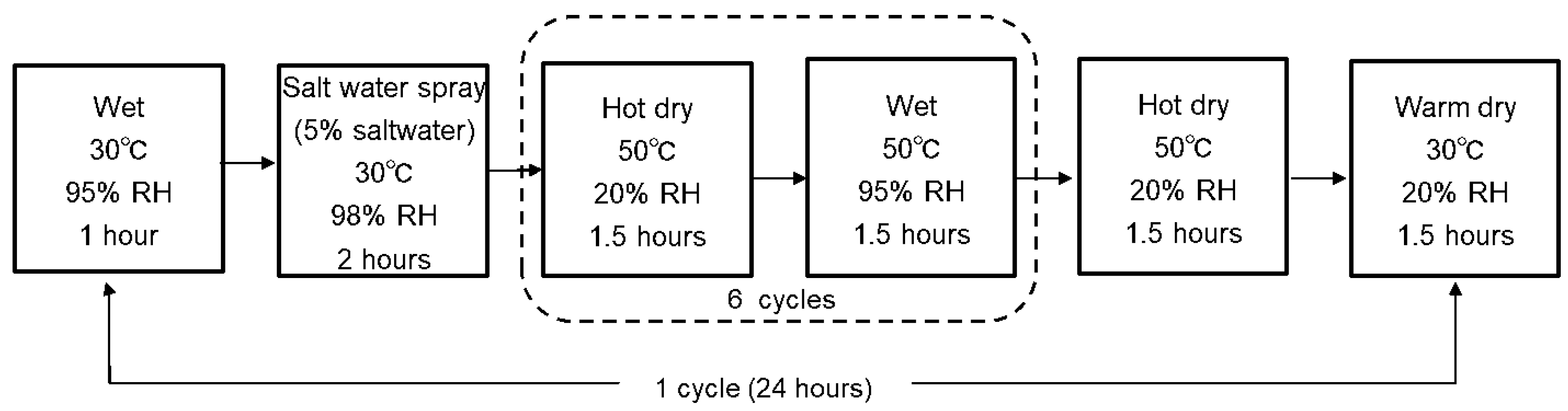
  29. Corrosion of Metals and Alloys—Accelerated Cyclic Corrosion Tests with Exposure to Synthetic Ocean Water Salt-Deposition Process—“Dry” and “Wet” Conditions at Constant Absolute Humidity. Available online: https://www.iso.org/obp/ui/#iso:std:iso:16539:ed-1:v1:en (accessed on 4 April 2022).
  30. Fujii, K.; Ohashi, K.; Kajiyama, H. Corrosion aspect of electrical appliances–development of new accelerated corrosion Test simulating appliances environment (1). Zairyo-to-Kankyo 2006, 55, 349–355. [Google Scholar] [CrossRef] [Green Version]
  31. Jiang, F.; Hirohata, M.; Liu, J.; Ojima, K. Application of accelerated cyclic Test with synthetic ocean water salt-deposition process to the evaluation on corrosion characteristics of weathering steel. Corros. Eng. Sci. Technol. 2022, 57, 1–10. [Google Scholar] [CrossRef]
  32. Chen, X.; Duan, Y.; Houthooft, R.; Schulman, J.; Sutskever, I.; Abbeel, P. Infogan: Interpretable representation learning by information maximizing generative adversarial nets. In Proceedings of the 30th International Conference on Neural Information Processing Systems, Kyoto, Japan, 16–21 October 2016; pp. 2180–2188. [Google Scholar]
  33. Mirza, M.; Osindero, S. Conditional generative adversarial nets. arXiv 2014, arXiv:1411.1784. [Google Scholar]
  34. Chollet, F. Xception: Deep Learning with Depthwise Separable Convolutions. arXiv 2016, arXiv:1610.02357. [Google Scholar]
  35. Zhang, J.; Zhuang, Y.; Ji, H.; Teng, G. Pig Weight and Body Size Estimation Using a Multiple Output Regression Convolutional Neural Network: A Fast and Fully Automatic Method. Sensors 2021, 21, 3218. [Google Scholar] [CrossRef] [PubMed]
  36. Huang, W.; Yang, C.; Hou, T. Spine Landmark Localization with combining of Heatmap Regression and Direct Coordinate Regression. arXiv 2020, arXiv:2007.05355. [Google Scholar]
Figure 1. The size of steel plates and corrosion measure area.
Applsci 12 04706 g001
Figure 2. The procedure of seawater spray experiment ISO16539.
Applsci 12 04706 g002
Figure 3. Organization of steel plates in PWRI.
Applsci 12 04706 g003
Figure 4. The procedure of PWRI.
Applsci 12 04706 g004
Figure 5. Atmospheric exposure experiments.
Applsci 12 04706 g005
Figure 6. System Architecture.
Applsci 12 04706 g006
Figure 7. Architecture of UNet.
Applsci 12 04706 g007
Figure 8. The Corrosion on ISO16539 Type SM400A Steel Plate Stage Three and Corresponding Simulated Corrosion. (a) The Corrosion on ISO16539 Type SM400A Steel Plate Stage Three; (b) The Corrosion on Simulated Type SM400A Steel Plate Stage Three.
Applsci 12 04706 g008
Figure 9. The Corrosion on ISO16539 Type SM490A Steel Plate Stage Three and Corresponding Simulated Corrosion; (a) The Corrosion on ISO16539 Type SM490A Steel Plate Stage Three; (b) The Corrosion on Simulated Type SM490A Steel Plate Stage Three.
Applsci 12 04706 g009
Figure 10. The Corrosion on ISO16539 Type SMA400 Steel Plate Stage Three and Corresponding Simulated Corrosion; (a) The Corrosion on ISO16539 Type SMA400AW Steel Plate Stage Three; (b) The Corrosion on Simulated Type SMA400AW Steel Plate Stage Three.
Applsci 12 04706 g010
Figure 11. The Corrosion on ISO16539 Type SMA490AW Steel Plate Stage Three and Corresponding Simulated Corrosion; (a) The Corrosion on ISO16539 Type SMA490AW Steel Plate Stage Three; (b) The Corrosion on Simulated Type SMA490AW Steel Plate Stage Three.
Applsci 12 04706 g011
Table 1. Corrosion Dataset.
SubsetsISO16539PWRIAtmospheric Exposure IAtmospheric Exposure IITotal
Number of samples3616121276
Table 2. Chemical compositions and mechanical properties.
Chemical Compositions (Mass %)Mechanical Properties
CSiMnPSCuNiCrYield Stress (MPa)Tensile Strength (MPa)Elongation (%)
SM400A0.180.170.50.0150.006---27944229
SM490A0.160.021.040.0110.005---42654220
SMA400AW0.120.20.670.0150.0040.310.090.4930544533
SMA490AW0.120.221.140.0150.0020.310.090.4939151430
Table 3. Training set vs. Testing set.
Scenario 1Scenario 2Scenario 3Scenario 4Scenario 5Scenario 6
Training setds1ds1ds2ds2ds1 + ds2ds1 + ds2
Testing setds3ds4ds3ds4ds3ds4
Table 4. Comparative Results.
Train: ds1;
Test: ds3
Train: ds1;
Test: ds4
Train: ds2;
Test: ds3
Train: ds2;
Test: ds4
Train: ds1 + ds2; Test: ds3Train: ds1 + ds2; Test: ds4
GAN0.39170.4230.46190.33730.19760.2442
InfoGAN0.36840.4550.43280.3630.23310.3468
cGAN0.46630.46980.43850.45230.31320.2987
Baseline model: Xception0.95241.49230.8820.58730.90150.8837
Publisher’s Note: MDPI stays neutral with regard to jurisdictional claims in published maps and institutional affiliations.

