Numerical Investigation on a Liquid–Gas Ejector for Carbon Dioxide Removal Using Amine Solution: Hydrodynamics and Mass Transfer Evaluation

Abstract

The present study investigates the hydrodynamics and mass transfer of the liquid–gas ejector using three-dimensional (air–water) and two-dimensional (CO₂/air-MEA (Monoethanolamine) solution) computational fluid dynamics (CFD) modeling. For 3D simulation, validation of the CFD results of this ejector with experimental data (error less than 5%) showed high simulation accuracy. The effects of motive liquid flow rate and outlet pressure parameters on the air entrainment rate and air hold-up are also investigated. It was found that by increasing the outlet pressure by about 70% (from 3587 to 6127 Pag), the rate of gas entrainment and gas hold up decreased by about 37% and 20%, respectively. On the contrary, these parameters showed increasing behavior of about 74% and 15%, respectively, when the mass flow rate of liquid increased by about 21%. In addition, three-dimensional phenomena such as mixing shock and the location of its occurrence are examined, which is the reason for recirculation and vortex in the ejector. Next, by simulating a two-dimensional simulation and changing the inlet fluids to CO₂/air-methanol amine, the ejector was designed to simultaneously increase the gas pressure and absorb carbon dioxide. A user-defined function code was used to express the mass transfer from the gas to the liquid phase. The results, in this case, showed that with increasing the outlet pressure of the ejector (from 0 to 2000 Pag), and enhancing the concentration of MEA solution (from 10% to 30%), the CO₂ removal boosted from 83% to 95%. A similar behavior was shown when the L/G ratio increased from 3.5 to 5.5. This study serves as a showcase on how to do an exact design and analysis for liquid–gas ejectors in flare gas recovery systems.

1. Introduction

Liquid–gas ejectors, in which the secondary fluid is gas, have the potential to be used in carbon capture and storage. Ejectors are used to draw more fluid from wells in the oil and gas sector, helping to increase output and reduce costs. Ejectors are also used for post-combustion carbon capture in power plants, to improve external waste heat to reduce the quantity of turbine steam needed for solvent regeneration. In addition to gas compression, ejectors may also be used for refrigeration and CO₂ transportation and storage, and numerous studies have been done to analyze and improve their effectiveness [1].

One of the challenging issues that has always attracted the attention of the experts is how to control and reduce greenhouse gas emissions because of their vast negative environmental impacts [2]. Furthermore, due to the district regulations related to greenhouse gas emissions, experts and scholars have recently focused on the more efficient and clear processes in which the amount and type of the released gas are under control [3]. Due to the demand for hydrocarbon-based fuels, the oil and gas sectors play a pivotal role in the current situation. During the extraction process of gas and oil, some co-products are created that must be discharged into the surrounding environment. Burning the mentioned gaseous material in flare systems is a common method that is followed in gas and oil fields. Although burning the hazardous gaseous products in the flare systems boosts the safety of gas and oil fields and diminishes the internal pressure of the extraction systems, it has a catastrophic impact on the surrounding environment [4]. From economic and environmental standpoints, utilizing flare gas recovery units in the gas and oil fields has many merits, such as boosting production efficiency, decreasing operating costs and maintenance, and reducing noise and flare emissions [5].

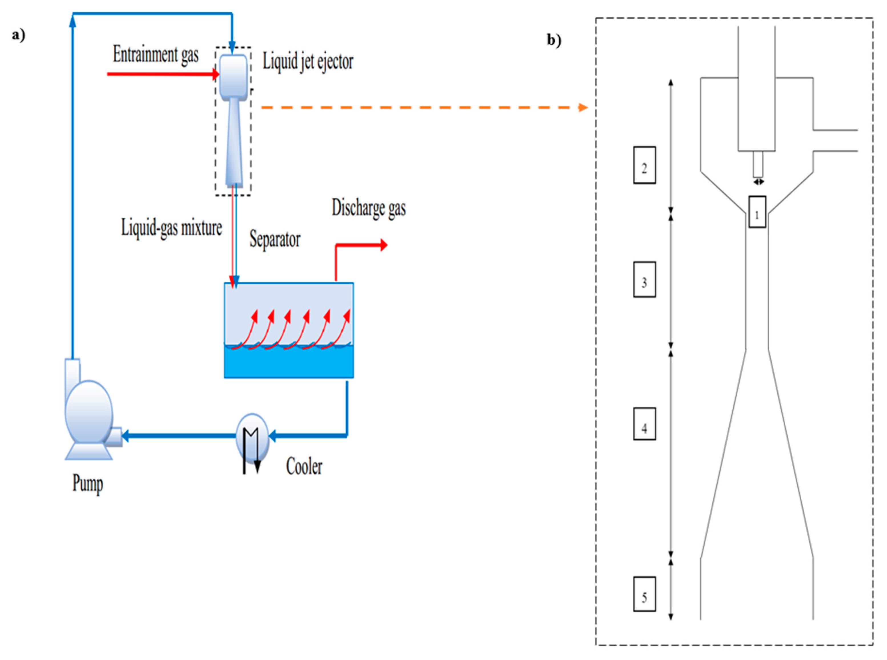
In the chemical-based processes that experts face with coaxial flow systems, ejectors are considered as one of the most critical elements in which a high-pressure current entrains a low-pressure current. This element is widely utilized in flare gas recovery units. To delve deeper into the role of the flare gas recovery unit, it should be highlighted that the recovery unit collects gases before entering to flare unit, and compressing and cooling them remarkably reduces the amount of discharged gas to the environment. The recovered gas extracted from the flare gas recovery unit is utilized as feed in other sections of the chemical plant. The common form of a flare gas recovery unit with a liquid-based ejector and a liquid–gas ejector’s geometry has been depicted in Figure 1. The general ejector includes, as shown in this Figure, a nozzle (1), a suction chamber/converging part (2), where one phase is injected into the system at a high rate of speed via a nozzle, and a low-pressure zone is created in accordance with Bernoulli’s principle, a throat (3), where the gas and liquid phases mix and a dispersion of gas and liquid is formed, a pressure recovery part (4), and a contactor (5) for providing gas–liquid contact.

Because the ejector is so crucial in the flare gas recovery unit, a lot of research has been done on it in both theoretical and experimental ways. In this regard, computational fluid dynamics is applied to evaluate the performance of ejectors in different conditions and different fluids [6,7,8]. For instance, Aidoun et al. [9] provided a review paper about the most recent innovations, advances, and novel applications of single-phase ejectors. A wide range of aspects of mentioned ejector were scrutinized. Moreover, the potential of the single-phase ejector to employ as a single equipment or integrate with other elements in a combined system was assessed. Two-phase ejectors are another type of ejector in which two different materials flow inside the ejector. The simulation of these types of ejectors was precisely reviewed by Song et al. [10]. Bauzvand et al. investigated the experimental and computational fluid dynamics of an ejector with a new geometry to improve its performance. The multi-nozzle and swirls effect features are combined in the proposed inlet geometry. With the applied changes, the ejector efficiency increased by 158% [11]. El-Zahaby et al. [12] tested the configuration of gas-gas ejectors based on numerical analysis. They considered different operation circumstances and geometries, and a CFD model was developed to assess the proposed system. The results demonstrated that the system’s performance is influenced by the current and character of the ejector. In another study [13], an innovative liquid-liquid ejector was hydrodynamically evaluated by CFD. The results of validation demonstrated that the simulation’s findings had enough accuracy. Moreover, some critical variables, such as jet velocity, column to nozzle diameter ratio, and two phases flow ratio, were selected, and their impacts on the proposed system’s efficiency were assessed. Patel et al. [14] conducted a numerical modeling of a multi-nozzle jet ejector using CFD. They evaluated three different sets of nozzles inside a jet ejector and compared the finding results. Additionally, they assessed the dynamic of break-up and bubble coalescence in the mentioned system by considering 3D numerical domains. Void fraction, velocity, and bubble size were three critical parameters tested in a dual-channel optical fiber probe in a liquid–gas annular ejector system by Aliyu et al. [15]. Based on the results and comparing them with experimental data, the accuracy of measured parameters was verified. A single phase model based on CFD was developed by Sharma et al. [16]. The authors simulated a gas–liquid nozzle to anticipate the gas induction rates. Additionally, the influences of variables such as the nozzle’s mixing length, the diameter of the nozzle, suction chamber geometry, etc., were scrutinized and reported. Operating circumstances are another critical parameter that was especially evaluated by Zheng et al. [17]. To this end, a two-phase CFD-based model was developed for an ejector. In that investigation, Liquefied natural gas (LNG) and Boiling Off Gas (BOG) were chosen as primary and secondary fluids inside the simulated ejector. The simulation’s results revealed that the phase change had a remarkable impact on the system’s efficiency. The fluid type inside the liquid jet ejector was another parameter tested by Sharma et al. [18]. Unlike other investigations in which the impacts of the turbulent phenomenon have been neglected, in that research, authors tried to evaluate the turbulence phenomena and its influences on the issues such as jet dynamic and rate of gas induction. They reported that the mentioned issue should be considered to reach a reliable and more correct CFD model. The mixing flow behavior and its impact on liquid–gas ejectors were modeled by Wang et al. [8]. The model was developed based on the realizable k–ε turbulence mode by ANSYS-FLUENT software. By simulating the system, all critical variables were investigated for the ejector. A great number of scholars and experts have been widely working on both the computational evaluations and experimental-based investigations around ejectors and their characteristics [19,20,21,22].

To the best of our knowledge, there has been no hydrodynamic study of carbon dioxide capture in an ejector in the literature prior to this study. The present work firstly evaluates the hydrodynamics of a 3D liquid–gas (water–air) ejector. In this study, the experimental values such as water flow rate and separator pressure are used from the experimental work by Mandal [23]. The impacts of motive liquid flowrate and outlet pressure on the air entrainment rate and air hold-up were assessed using 3D CFD simulation. One of the important research gaps that has been neglected in other similar investigations is related to mixing shock and where it occurs. In the current study, the authors evaluated the 3D geometry of the simulated ejector with considering mixing shock. 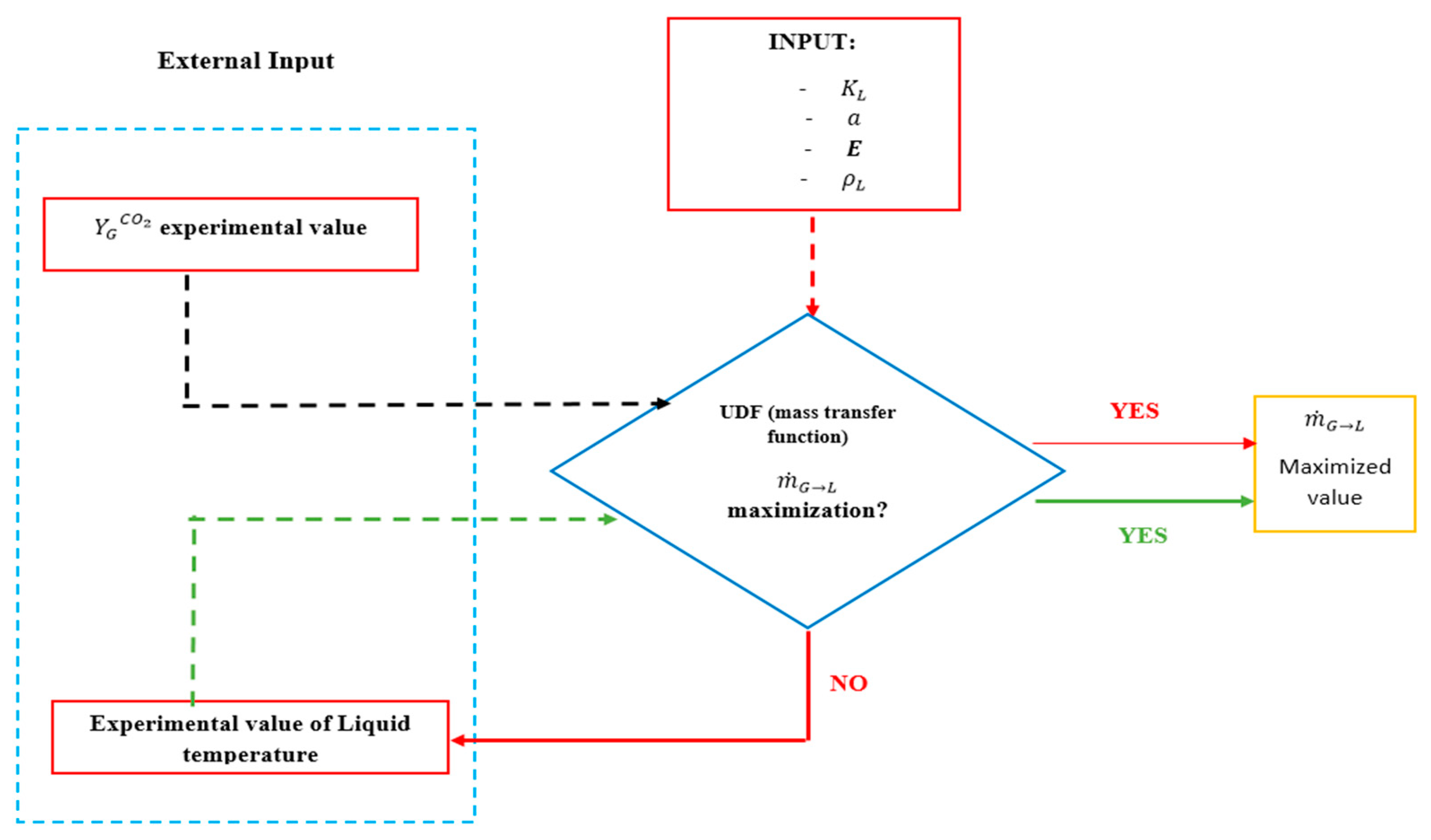After evaluating the 3D geometry and finding its reliability and accuracy, hydrodynamic and mass transfer of a dual function ejector are assessed in a 2D liquid–gas (MEA solution–CO₂/air) ejector for simultaneously increasing gas pressure and capturing CO₂. This action is performed to assess the mass transfer through the liquid–gas ejector by using User-Defined Function (UDF) code. The mixture of carbon dioxide and air is selected as the gas phase, and the amine solution plays the liquid phase’s role in the 2D evaluation. The effects of ejector outlet pressure, amine concentration, and liquid-to-gas (L/G) ratio on the CO₂ removal are evaluated by using 2D CFD modeling. In all stages, grids and mesh independency, Eulerian–Eulerian approach as a multiphase model, and Standard k-$\epsilon$ model as the turbulent behavior model of the flow, are implemented. The commercial CFD package ANSYS-FLUENT 17 is the software that is used to conduct this investigation.

2. Modeling Approach

Two common approaches exist for the numerical modeling of multiphase flows. One is Eulerian–Lagrangian method. The other is the Eulerian–Eulerian approach. In the first method, the dispersed phase is considered as an independent discrete phase. In order to solve the dispersed phase, a large number of particles, bubbles, or droplets must be calculated through the computed flow field. Furthermore, momentum, mass, and energy exchanges between the dispersed and fluid phases can be done effectively. On the contrary, the second method considers both phases (fluid and dispersed) as two continuous phases that continuously penetrate to each other. For each phase (not for each one of bubbles, droplets, or particles in the dispersed phase), governing equations are made up of a set of relationships that are uniform in structure for all phases [24]. Since each particle, bubble, or droplet is tracked in a Lagrangian framework, the Eulerian–Lagrangian approach is computationally intensive. In addition, in this approach, owing to the convergence problem at higher hold-ups, the secondary phase should not exceed ten percent of the total volumetric flow rate. In the majority of cases, the volume fraction of the dispersed phase is more than ten percent; therefore, the more common model in CFD is based on the Eulerian–Eulerian approach. In this study, a three- and two-dimensional modeling with considering Eulerian–Eulerian approach is implemented, in which gas phase/liquid phase for 3D and 2D simulation are air/water and CO₂ + air/MEA solution, respectively. The liquid phase is considered as a continuous phase, but the gas phase is regarded as a dispersed fluid phase with a constant bubble diameter (1 mm). The turbulent behavior of the flow was modeled using a standard k-$\epsilon$ model. Some assumptions are made in this simulation: (1) the flow conditions are isothermal (25 °C) and (2) the virtual mass force is neglected.

2.1. Continuity and Momentum Equations

The governing equations of the 3D ejector (water–air) include continuity and momentum equations. For the 2D (MEA solution–CO₂/air) ejector, due to the presence of MEA and CO₂, the species transport equation is also added.

The dimensional unsteady-state governing fluid flow equations of phase k are presented in Equations (2) and (3). Additionally, in the Eulerian–Eulerian approach, the term of volume fraction is shown. It is assumed that at a specified time, a volume fraction of phase k, (${\alpha }_k$), exists in a small place. If there are n phases in total, Equation (1) is obtained:

$${\sum }_{k=1}^n{\alpha }_k=1$$

(1)

This means that a large number of particles of diverse phases exist in a volume that is defined by the macroscopic length of the system, in which the sum of the volume fraction is equal to one. The continuity equations and momentum formulations are presented by the two following equations [25,26]:

$$\frac{\partial ({\alpha }_k{\rho }_k)}{\partial t}+\nabla .({\alpha }_k{\rho }_k{u}_k)=-{\dot{m}}_{k\to l}$$

(2)

$$\frac{\partial ({\alpha }_k{\rho }_k{u}_k)}{\partial t}+\nabla .({\alpha }_k{\rho }_k{u}_k{u}_k+{\alpha }_k{\tau }_k)={\alpha }_k{\rho }_{k}g-{\alpha }_k\nabla p+M_k-{\dot{m}}_{k\to l}{u}_k$$

(3)

where ${\alpha }_k$ is the volume fraction of phase k, ${\rho }_k$ is the density of phase k, $u_k$ is the velocity of phase k, $g$ is the acceleration of gravity, $p$ is the pressure, $t$ is time,${\dot{m}}_{k\to l}$ shows the rate of mass transfer from the kth phase to the liquid phase that is zero for 3D simulation, and $M_k$ demonstrates the total interfacial forces.

In the above formula, ${\tau }_k$ denotes the shear stress in the kth phase and is calculated by the following equation [25]:

$${\tau }_k=-{\mu }_{k,eff}\left[\left((\nabla u_k)+{(\nabla u_k)}^T\right)-\frac{2}{3}I(\nabla .u_k)\right]$$

(4)

where ${\mu }_{k,eff}$ shows the effective viscosity and presents a summation of molecular and turbulent viscosities.

2.1.1. Interfacial Forces

To effectively predict the gas distribution, it is necessary to take the interface forces, such as drag, lift, wall lubrication, turbulent dispersion, and virtual mass, into account. Compared to other interfacial forces, the virtual mass force had minimal impact on the results [27]. Consequently, the virtual mass force is left out of the equation. Interfacial forces are denoted by the following expression:

$$M_k=\overrightarrow{F_D}+\overrightarrow{F_{lift}}+\overrightarrow{F_{td}}+\overrightarrow{F_{wl}}$$

(5)

The drag, lift, turbulent dispersion, and wall lubrication forces are denoted by ${\mathrm{F}}_{\mathrm{D}}$, ${\mathrm{F}}_{\mathrm{lift}}$, ${\mathrm{F}}_{\mathrm{td}}$, and ${\mathrm{F}}_{\mathrm{wl}}$.

Drag Force

The drag force is the result of hydrodynamic friction between the liquid and the dispersed phase, which means that particles move in liquid face resistance from this source. The drag force is defined as follows:

$$\overrightarrow{F_D}=\frac{3}{4d_b}{C}_D{\alpha }_G{\alpha }_L{\rho }_L|\overrightarrow{u_G}-\overrightarrow{u_L}| (\overrightarrow{u_G}-\overrightarrow{u_L})$$

(6)

where the slip velocity is ($(\overrightarrow{{\mathrm{u}}_{\mathrm{G}}}-\overrightarrow{{\mathrm{u}}_{\mathrm{L}}})$) and C_D is the coefficient of drag. C_D is largely determined by the Reynolds number (Re) for spherical bubbles. The C_D of non-spherical bubbles is determined by the Eötvös number (Eo). A formula for calculating the drag coefficients of various bubble shapes is presented [28]. When the bubbles’ Reynolds numbers are low, the bubbles retain their spherical shape, and C_D can be determined using C_D,sphere. However, as the bubbles’ Reynolds number is increased, the bubbles deform and take on the appearance of a cap bubble or an ellipse. The CD’s equivalent expression is as follows:

$$C_D=\max (\min (C_{D,ellipse}, C_{D,cap}), C_{D,sphere})$$

(7)

$$C_D=\{\begin{array}{cc}\frac{24}{Re} & Re<0.01\\ 24 (1+0.15R{e}^{0.687})/Re& Re\ge 0.01\end{array}$$

(8)

$$C_{D,ellipse}=\frac{4g{d}_b ({\rho }_L-{\rho }_G)}{3U_t{}^2{\rho }_L}$$

(9)

$$C_{D,cap}=\frac{8}{3}$$

(10)

where $d_b$ denotes the diameter of the bubble and $U_t$ denotes the settling velocity of the bubble.

Lift Force

A lift force is experienced by the particle when the liquid is flowing at a shear rate or rotates at a rotational rate [29]. The lift force is the primary cause of the void fraction’s uneven radial distribution in the dispersed phase, which is necessary to take into account when simulating the effect. The general expression is written as [30]:

$$\overrightarrow{F_{lift}}=-C_L{\alpha }_G{\rho }_L (\overrightarrow{{\mathrm{u}}_{\mathrm{G}}}-\overrightarrow{{\mathrm{u}}_{\mathrm{L}}})\times (\nabla \times \overrightarrow{{\mathrm{u}}_{\mathrm{L}}})$$

(11)

where $C_L$ is the lift force coefficient. Tomiyama et al. [31] carried out the experiment in an air–water system and found a correlation between the coefficient of lift and a modified Eo number when the change in bubble shape was taken into account. The coefficient of the lift force is defined as:

$$C_L =\{\begin{array}{c}\min [0.288\tanh (0.121 R{e}_b), f(E{o}^{\prime })] E{o}^{\prime }\le 4\hfill \\ f(E{o}^{\prime }) 4<E{o}^{\prime }\le 10\hfill \\ -0.27 10<E{o}^{\prime }\hfill \end{array}$$

(12)

where $R{e}_b$ is defined as ${\rho }_L{d}_b|\overrightarrow{u_G}-\overrightarrow{u_L}|/{\mu }_L$.

$$f(E{o}^{\prime })=0.00105E{o}^{\prime }{}^3-0.0159E{o}^{\prime }{}^2-0.0204E{o}^{\prime }+0.474$$

(13)

$$E{o}^{\prime }=\frac{g({\rho }_L-{\rho }_G)d_h{}^2}{\sigma }$$

(14)

where $E{o}^{\prime }$ is the modified $Eo$ number, $\sigma$ is the coefficient of surface tension, and $d_h$ is the maximum horizontal dimension of the bubble, which can be derived using following equation [32]:

$$d_h=d_b{(1+0.163 E{o}^{0.757})}^{1/3}$$

(15)

where $Eo$ is the Eötvös number. The magnitude of the lift coefficient is proportional to $Eo$. When the $Eo$ is small, the lift coefficient is greater than zero, and the bubbles retain their spherical form and migrate to the pipe wall. At high $Eo$, on the other hand, the lift coefficient is smaller than zero, causing the bubbles to deform and flow toward the pipe’s center.

Turbulent Dispersion Force

A consistent distribution of the dispersed phase occurs as a consequence of the force of turbulent dispersion, which takes into account the interaction between turbulent eddies and the particles they contact with.

An equation for the interphase drag term’s average time value may be generated by using the following formula [33]:

$$\overrightarrow{F_{td}}=\frac{3}{4}{C}_{TD}{C}_D\frac{{\alpha }_G{\alpha }_L}{d_b}|\overrightarrow{{\mathrm{u}}_{\mathrm{G}}}-\overrightarrow{{\mathrm{u}}_{\mathrm{L}}}|\frac{{\mu }_t}{{\sigma }_{TD}}(\frac{\nabla {\alpha }_G}{{\alpha }_G}-\frac{\nabla {\alpha }_L}{{\alpha }_L})$$

(16)

where C_TD is a constant that can be changed by the user and it is set to 1 and σ_TD is the turbulent Prandtl number which is 0.9. The turbulent dynamic viscosity is denoted by µ_t.

Wall Lubrication Force

In order to ensure that the bubbles do not touch the wall, the wall lubrication force acts as a barrier [34]. The wall lubricating force is expressed as:

$$\overrightarrow{F_{wl}}=-C_{WL}{\alpha }_G{\rho }_L{|\overrightarrow{{\mathrm{u}}_{\mathrm{L}}}-\overrightarrow{{\mathrm{u}}_{\mathrm{G}}}|}^2\overrightarrow{n_w}$$

(17)

where $\overrightarrow{n_w}$ represents the unit normal that points away from the wall and $C_{WL}$ denotes the coefficient of wall lubrication force. The following is an expression for C_WL [34]:

$$C_{WL}=max\left\{0, \frac{C_{w1}}{d_b}+\frac{C_{w2}}{y_w}\right\}$$

(18)

where $y_w$ is the distance to the wall.

2.2. Species Transport Equation

In this study, to observe the changes in the concentration of carbon dioxide in the gas phase, it is necessary to consider the species transport equation in the gas phase [25]:

$$\frac{\partial ({\alpha }_G{\rho }_G{Y}_G{}^{C{O}_2})}{\partial t}+\nabla .({\alpha }_G{\rho }_G{u}_G{Y}_G{}^{C{O}_2}-{\alpha }_G{\Gamma }_G{}^{C{O}_2}\nabla Y_G{}^{C{O}_2})=-{\dot{m}}_{G\to l}$$

(19)

In this equation, ${\Gamma }_G$ shows the diffusion coefficient,${\alpha }_G$ is the volume fraction of gas that is defined based on C_VOF (cell, gas) function, ${\rho }_G$ is the gas density that is defined based on C_R (cell, gas) function, $u_G$ is the gas velocity, $Y_G{}^{C{O}_2}$ is the CO₂ mass fractions in the gas phase, and $-{\dot{m}}_{G\to l}$ is the mass transfer of CO₂ from the gas to liquid phase that is determined by Equation (20) [25,35]. 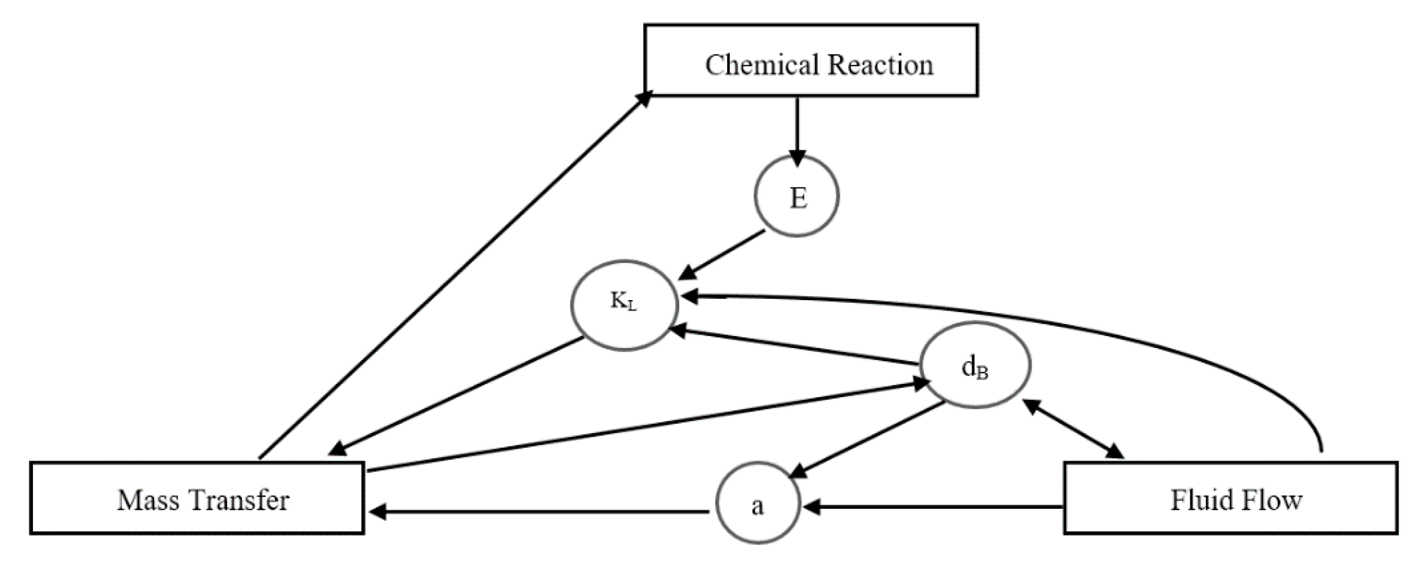As shown schematically in Figure 2, chemical reactions in a gas–liquid system include extremely complicated interconnections between the main processes. The pace of chemical reaction is regulated by the local concentration of the species and the mixing caused by the interphase mass transfer mechanism and scattered bubbles. The mass transfer coefficient, meanwhile, is a function of local hydrodynamics, which is itself impacted by bubble shrinkage as a result of physical or chemical absorption, as well as differences in physical characteristics as a result of inhomogeneous distributions of chemical species [36].

$${\dot{m}}_{G\to l}=K_{L}aE{\rho }_L(Y_l{}^{C{O}_2\ast }-Y_L{}^{C{O}_2})$$

(20)

where $K_L$ shows the overall mass transfer coefficient of liquid phase, $a=\raisebox{1ex}{$6{\alpha }_G$}\!\left/ \!\raisebox{-1ex}{$d_B$}\right.$ is interfacial area per unit volume, $d_B$ is bubble diameter that is equal to 1 mm, and $Y_L{}^{C{O}_2}$ and $Y_G{}^{C{O}_2}$(=0.191) are CO₂ mass fractions in liquid and gas phases, respectively. Due to the point that there is a mass transfer resistance in the liquid phase, with respect to Henry’s law, the mass fraction of liquid phase that is in equilibrium with the mass fraction of the gas phase is calculated by [25,35]:

$$Y_l{}^{C{O}_2\ast }=H^{C{O}_2}{Y}_G{}^{C{O}_2}\frac{{\rho }_G}{{\rho }_L}$$

(21)

In this study, the value of $H^{C{O}_2}$(=0.64) has been considered based on the data of an investigation carried out by Penttilä et al. [37] and ${\rho }_G$ and ${\rho }_L$ are gas and liquid densities that are defined based on C_R (cell, gas) and C_R (cell, liq) functions, respectively.

Additionally, in Equation (6), the enhancement factor $E$ is a constant related to chemical reactions and should be considered in calculations. In this study, this term is determined for modeled system via [25,35]:

$$E_{C{O}_2}={\left(\frac{D_{CO2,liq}}{D_{MEA,liq}}\right)}^{1/2}+{\left(\frac{D_{MEA,liq}}{D_{CO2,liq}}\right)}^{1/2}\frac{C_{MEA}}{v C_G{}^{C{O}_2\ast }}$$

(22)

where $v$ = 1 denotes the stoichiometry coefficient for CO₂ based on the reaction between CO₂ and MEA as follows:

$$C{O}_2(l)+2HO{C}_2{H}_{4}N{H}_2\to HO{C}_2{H}_{4}N{H}_3{}^{+}+HO{C}_2{H}_{4}NHCO{O}^{-}.$$

(23)

$C_{MEA}$ = 4.86 kmol/m³ is the concentration of MEA; besides, the diffusivity constant for CO₂ in the MEA ($D_{CO2,liq}$) is calculated by N₂O analogy, that is $6.7\times {10}^{-10}$ m²/s [38], while the diffusivity constant for MEA in water ($D_{MEA,liq}$) is considered based on data of Maceiras et al., which is equal to $1.12\times {10}^{-10}$ m²/s [39].

Additionally, $K_L$ is overall mass transfer coefficient in the liquid phase that is calculated for bubble movement based on the Sherwood relationship by H. Brauer [40]:

$$Sh=\frac{K_L{d}_B}{D_{C{O}_2}}=2+0.015 R{e}^{0.89}S{c}^{0.7}$$

(24)

where $d_B$ is the bubble diameter, $D_{C{O}_2}$ is the diffusivity for CO₂, $Re=\frac{{\rho }_L{V}_{rel}{d}_B}{{\mu }_L}$ is the Reynolds number, and $Sc=\frac{{\mu }_L}{{\rho }_L D_{CO2,L}}$ is the Schmidt number. Thus, $K_L$ is determined by the following relation:

$$K_L=\frac{D_{CO2,L}(2+0.015 {\left(\frac{{\rho }_L{V}_{rel}{d}_B}{{\mu }_L}\right)}^{0.89}{\left(\frac{{\mu }_L}{{\rho }_L{D}_{CO2,L}}\right)}^{0.7})}{d_B}$$

(25)

where $V_{rel}$ is the relative speed, ${\rho }_L$ is the liquid density, and ${\mu }_L$ is the liquid viscosity.

2.3. Turbulence Model

The turbulence model that is chosen has a significant impact on the outcomes of simulation, since it defines the liquid’s distribution of velocity. By solving two independent transport equations, two-equation turbulence models can determine both a turbulent length and time scale. Since the ejector contains turbulent flows with high Reynolds number, it is better to use standard $k-\epsilon$ and realizable $k-\epsilon$ models for the existing ejector. Because of the rotational effects, the $k-\epsilon$ realizable model is expected to perform better, but the standard $k-\epsilon$ model is chosen because it is simpler and requires less computational time than the $k-\epsilon$ realizable model. The standard $k-\epsilon$ model [41] is a model based on model transport equations for the turbulence kinetic energy (k) and its dissipation rate ($\epsilon$). The exact equation and physical reasoning are used to derive the model transport equation for k and $\epsilon$, respectively. Transport equations for the standard $k-\epsilon$ model, are given by:

$$\frac{\partial }{\partial t}(\rho k)+\frac{\partial }{\partial x_i}(\rho K{u}_i)=\frac{\partial }{\partial x_j}\left[\left(\mu +\frac{{\mu }_t}{{\sigma }_k}\right)\frac{\partial k}{\partial x_j}\right]+G_k+G_b-\rho \epsilon -Y_M+S_K$$

(26)

$$\frac{\partial }{\partial t}(\rho \epsilon )+\frac{\partial }{\partial x_i}(\rho \epsilon v_i)=\frac{\partial }{\partial x_j}\left[\left(\mu +\frac{{\mu }_t}{{\sigma }_{\epsilon }}\right)\frac{\partial \epsilon }{\partial x_j}\right]+C_{1\epsilon }{G}_k\frac{\epsilon }{k}-C_{2\epsilon }\rho \frac{{\epsilon }^2}{k}+S_{\epsilon }$$

(27)

$$G_k={\mu }_t \left(\frac{\partial u_i}{\partial x_j}+\frac{\partial u_j}{\partial x_i}\right)\frac{\partial u_i}{\partial x_j}$$

(28)

$$G_b=\beta g_i\frac{{\mu }_t}{P{r}_t} \frac{\partial T}{\partial x_i}$$

(29)

$${\mu }_t={\rho }_L{C}_{\mu }\frac{k^2}{\epsilon }$$

(30)

$$S=\sqrt{2{\mathrm{S}}_{\mathrm{ij}}.{\mathrm{S}}_{\mathrm{ij}}}$$

(31)

$$S_{ij}=\frac{1}{2} \left(\frac{\partial u_i}{\partial x_j}+\frac{\partial u_j}{\partial x_i}\right)$$

(32)

where G_k denotes the kinetic energy generated by turbulence as a result of the average velocity gradients. The buoyancy-induced generation of turbulence kinetic energy is denoted by G_b. In compressible turbulence, Y_M is the effect of the fluctuating dilation. S_K and $S_{\epsilon }$ are source terms. $C_{1\epsilon }$ = 1.42, $C_{2\epsilon }$ = 1.92, $C_{\mu }$ = 0.09, and $\beta$ = 0.012 are constants. ${\sigma }_k$ = 1 and ${\sigma }_{\epsilon }$ = 1.3 are the turbulent Prandtl numbers for k and $\epsilon$. S is the tensor of deformation and S_ij is the mainstream time strain rate. The initial values of turbulent kinetic energy (k) and turbulent dissipation rate ($\epsilon$) for air and water are considered 1 m²/s² and 0.22 m²/s³, respectively.

2.4. Geometries, Grids, and Mesh Independency

In this study, for the computational domain and grid generation, Fluent Meshing software is used. The dimensions of geometry are shown in

Table 1. Dimensions of the liquid–gas ejector [42].

Description	Dimension (mm)
Height of the suction chamber	50
Diameter of suction chamber	60
Diameter of throat	19
Length of the throat	183
Length of the diffuser	254
Diameter of the contactor	60
Diameter of gas inlet	10
Length of the contactor	25
Diameter of the nozzle used	6

and Figure 3 [42]. Additionally, 3D and 2D solution domain with uniform mesh is shown in Figure 3. Due to the mixing shock, the concentration of grid density is centered on the exit of nozzle and also the throat. To acknowledge the stability of numerical results (mesh independency), the ejector with 3D design and d_nozzle = 12 mm is selected. The effect of three sets of grids (i.e., 107,793, 206,537, and 387,987 mesh elements) on the air entrainment rate, Q_g, at motive liquid flow rate (Q_L = 2.17 × 10⁻⁴ m³/s) is listed in

Table 2. Investigation of mesh independency of the designed 3D and 2D liquid–gas ejector.

	Total Cell Amount			Parameter
	107,793	206,537	387,987
3D geometry	2.4	2.4	2.4	CPU (2.4 GHz and 8 cores)
	6	9	14	Time (day)
	20	6	6	Error: $(\frac{|Q_{g,Experimental}-Q_{g,\mathrm{CFD}}|}{Q_{G,Experimental}}\times 100)$
2D geometry	40,780	60,234	75,325
	2.4	2.4	2.4	CPU (2.4 GHz and 8 cores)
	1	2.5	4	Time (day)
	23	7	7	Error: $(\frac{|Q_{g,Experimental}-Q_{g,\mathrm{CFD}}|}{Q_{G,Experimental}}\times 100)$

. The error percentage is calculated by obtaining air entrainment rate for each grids and comparing it with experimental data [23]. It can be seen that the results achieved for grids with 206,537 and 387,987 cells confirm the stability of numerical results; however, the grid with 206,537 cells needs less computational time than the one with the 387,987 cells. Therefore, the grid with 206,537 cells was selected for this section.

The predicted outcomes could be significantly affected by the bubbles’ diameter. Based on the experimental work done by Mandal [23], which is the basis of this study, an asymmetry toward larger bubble sizes was observed in the bubble size distributions, which differed from a normal distribution. Thus, according to this paper, we chose d_b = 1 mm as the model parameter for the simulation. It is noted that d_b = 1 mm is also used for the independency of grid.

To investigate the absorption of carbon dioxide by MEA inside the ejector, due to the existence of mass transfer and enhancing the convergence and analyzing time, a 2D-axisymmetric geometry has been considered with a quadrilateral and triangular-meshing scheme. For two-dimensional geometry, similar procedures to the three-dimensional geometry were applied, and the grid with 60,234 cells was selected. The results are shown in Table 2. Additionally, a 2D solution domain with uniform mesh is shown in Figure 3.

2.5. Fluid Properties and Boundary Conditions

In this work, for 3D simulation, air and water are, respectively, used as gas and liquid phases; the characteristics of those are listed in

Table 3. Fluid properties of the designed 3D liquid–gas ejector.

Fluid	Density (kg/m3)	Viscosity (kg/m·s)	Surface Tension (N/m)
Water	997	0.00091	-
Air	1.168	1.86 × 10−5	-
Water–air	-	-	0.072
CO2	1.784	1.919 × 10−5
MEA	999.83	0.018

. A velocity inlet boundary condition is applied to the water inlet zone (nozzle section). Since the other inlet boundary zone for air is open to the atmosphere, the inlet zero-gauge pressure is exerted to this boundary (suction section). According to the research done by Mandal [23], at the ejector outlet, a 3250 Pa static gauge pressure ($P_{gauge}$) is used. A no-slip wall boundary condition is specified on the wall. The symmetry boundary condition is introduced for all of perpendicular faces.

For 2D simulation, the mixture of air and CO₂ is used as gas phase and MEA solution is used as liquid phase. The properties of these fluids are shown in Table 3. The boundary conditions that are considered in the simulation process of 2D ejector are reported in

Table 4. The boundary conditions of the simulated 2D ejector.

Position	Type of Boundary Condition
Walls	Adiabatic and non-slip
Inlet liquid	velocity inlet + mass fractions of components (30% amine solution)
Inlet gas	Pressure inlet + mass fractions of components (19.1% CO2 and 80.9% air)
Outlet flow	Pressure outlet
Symmetry	Axis

.

2.6. Algorithm

All numerical simulations in this study are carried out under non-steady-state conditions. FLUENT 17.0 commercial software is used to predict the distribution of the two phases. Volume fraction is discretized using the QUICK method. The First Order Upwind scheme was used for other equations. Additionally, the SIMPLE scheme was exerted for the pressure–velocity coupling. For all the simulations done in the present work, the convergence criteria for the solutions are considered when the achieved residuals are less than 1 × 10⁻³. One of the important parameters that affects the convergence criteria of simulation is the under-relaxation factor. The under-relaxation factor minimizes oscillations and contributes to the stability of the computation. In this study, under-relaxation factors for pressure, density, momentum, volume fraction, turbulent kinetic energy, and turbulent dissipation rates are considered 0.3, 1, 0.7, 0.2, 0.8, and 0.8, respectively.

3. Results and Discussion

3.1. Results of 3D CFD Modeling of Liquid–Gas Ejector

3.1.1. Validation and the Effect of Different Parameters on Gas Entrainment Rate

The experimental and predicted values of gas entrainment rate as a function of water flow rate and separator pressure in the liquid–gas ejector with 6 mm nozzle diameter are shown in Figure 4a,b. These figures evidently show that the experimental values attained for gas entrainment [23] are consistent with the predicted ones. Furthermore, Figure 4a demonstrates that the gas entrainment rate increases with liquid flow rate. This increment can be justified by the fact that an increment in water flow rate leads to an increase in driving force. This ejector’s pressure drop is the primary driving force for gas entrainment that is a pressure difference between the beginning and end of the nozzle ($\mathsf{\Delta }p$). The greater the pressure difference, the more liquid can be entrained into the ejector. Moreover, the momentum transfers from water to air, and consequently, air entrainment rate increases. At high liquid flow rates, the driving force remains approximately constant; therefore, gas entrainment rate does not change. Figure 4b shows the relationship between separator pressure and gas entrainment at a constant liquid flow rate of 2.85 × 10⁻⁴ m³/s. The findings reveal that the gas entrainment rate reduces with increasing separator pressure when the liquid flow rate remains constant. If the separator pressure increases, the entrained gas bubbles have more difficulty moving downward in the ejector, resulting in lower entrainment.

3.1.2. The Effect of Different Parameters on Gas Phase Hold-Up

The effects of liquid flow rate and separator pressure on gas phase hold-up in ejector are depicted in Figure 5a,b, respectively. These results are obtained by drawing several vertical lines from the beginning (z = 0 mm) to the end of the ejector (z = 512 mm) and averaging the gas hold-up along these lines by Fluent software. It is clearly observed that gas phase hold-up increases by enhancing the liquid flow rate, which results in an increment in the nozzle velocity and more gas entrains, which in turn increases gas hold-up. On the contrary, by increasing the separator pressure, less gas entrains, leading to a decrease in gas phase hold-up. Because our research has numerically investigated the performance of two-phase ejector by CFD method under transient condition, variation of gas phase hold-up with time is shown in Figure 6. The coefficient of mass transfer is proportional to the gas phase hold-up [43], so by increasing the gas phase hold-up over time, the mass transfer rate increases too.

3.1.3. Recirculation and Vortex

The CFD simulation can predict the internal flow regimes in the liquid–gas ejector, as shown in Figure 7a. According to this Figure, air is entrained by a water jet into the mixing chamber. The gas and liquid are in contact with each other in mixing tube and then liquid–gas mixture is discharged through the diffuser. The magnified interface around the mixing chamber (Figure 7b) shows that a recirculation zone occurs and the vortex is generated in this section that immediately disappears in the diffuser [44]. The main reason that causes the creation of recirculation zone is the influence of mainstream on circular jet. With mixing the mainstream and circular jet bends, a fan-shaped flow trajectory is made. The mentioned created flow acts like an umbrella to become an aerodynamic barrier in the current field, behind which a negative pressure zone is created, and due to this phenomenon, a recirculation zone is made that is shown in Figure 8.

3.1.4. Ejector Performance and the Effect of Liquid Flow Rate on Negative Pressure

Figure 9 shows the pressure and velocity contour inside the liquid–gas ejector. It can be seen from these contours that the maximum flow velocity takes place at the exit of the nozzle. Additionally, momentum exchange and mixing with the secondary fluid stream decrease the velocity. Another noteworthy finding is that the effects of boundary layer give rise to a velocity gradient from the wall to the center line flow of the ejector. At the nozzle’s exit, the view depicts the transformation of pressure energy to kinetic energy. There is also pressure energy generated in the diffuser section from the remaining kinetic energy. Negative pressure is a criterion for evaluation of the performance of ejector. The negative pressure formed when the fluid passes through the narrow throat enables the self-entrainment of ambient air into the channel. In this regard, we investigated the relationship between negative static pressure and liquid flow rate. Figure 10 illustrates that at higher liquid flow rate (2.49 × 10⁻⁴ m³/s to 2.64 × 10⁻⁴ m³/s), more negative pressures are observed in broader area, which is in agreement well with observation in literature reported by Opletal et al. [46]. By enhancing the mass flow rate of liquid, the outlet velocity of the ejector increases. This increment has a direct impact on the creation of negative pressure zone in this position. Under other conditions, the greater the speed, the greater the negative pressure.

3.1.5. Mixing Shock and Location of Its Occurrence

In the annular entrance zone, no changes are essentially found in both streams, whereas a gas boundary layer begins to develop on the wall and interfacial shear forces act between the surface of the jet and the gas annulus. A critical magnitude is reached for the wave disturbances on the jet inside the throat, but prior to the mixing zone, high-velocity droplets are shed from the jet into the annular space. The position of the mixing shock zone is an important factor for evaluating the performance of the ejector. By knowing the location of mixing shock, it is possible to know in which area of the ejector the liquid jet is broken. The plot of static pressure profile of the ejector (along its centerline) and contour of volume fraction of air in the ejector are shown in Figure 11a,b, respectively. As it is evident from these figures, due to the mixing shock, a decrease and an increase are observed, respectively, in the volume fraction of air and static pressure at the end of the mixing tube; therefore, mixing shock comes about in this region and liquid jet breaks up just at the end of the mixing tube. It shows that the nozzle is situated at an optimum position.

3.1.6. The Influence of the Mass Flow Rate on the Mixing Shock Phenomenon

In Figure 12, pressure contours along the ejector for the specific mass flow rates of (a): 2.49$\times {10}^{-4}$ and (b): 2.64 $\times {10}^{-4}$ m³/s are depicted. As mentioned in Section 3.1.5, mixing shock occurs where a decrease in pressure is observed (red arrows). As is crystal clear, with increasing the mass flow rate of the liquid, the mixing shock is transferred from the ejector throat to the diffuser side. In this position, increased mass flow rate causes an enhancement in the velocity of the gas film around liquid jet. Therefore, the location of the mixing shock that depends on the velocity of the annular gas flow is transferred downwards, and a considerable amount of kinetic energy that is related to this flow is lost in this shock.

3.2. Results of 2D CFD Modeling of the Liquid–Gas Ejector

In this part, after witnessing that the model obtained good results in 3D mode, a CFD-based 2D liquid–gas ejector, considering mass transfer phenomena, was simulated. The mass transfer between the two phases is determined by the two-phase interactions. Since in this study, the mass transfer does not operate at a uniform rate and depends on various factors such as the concentration of the target component in the target phase, mass transfer between two phases is determined by using the in-house subroutines called User-Defined Functions code that its flow chart is shown in Figure 13. A user-defined function, or UDF, is a function written in the C programming language that may be dynamically loaded into the ANSYS-Fluent solver to extend its standard capabilities. Function declarations provided by ANSYS-Fluent are used to define UDFs. Macros are used to implement these function declarations in the code. In this study, DEFINE_MASS_TRANSFER macro is used for defining CO₂ mass transfer rate from gas to liquid phase. The UDF includes several functions in its subset, such as C_VOF (cell, gas) for the volume fraction of gas, C_R (cell, liq) for the liquid density, and C_V (cell, gas) for the velocity of the gas phase.

3.2.1. The Impact of Ejector’s Outlet Pressure on the Removal of CO₂

The impacts of ejector outlet pressure from 0 to 2000 Pag on the removal of CO₂ have been depicted in Figure 14. Removal percentages were determined using Equation (33). To calculate the mass fraction of carbon dioxide (Y_CO2), according to Figure 15, the ejector is divided into different parts, and the average mass fraction of each part is calculated.

$$\% C{O}_{2}removal=\frac{Y_{i,C{O}_2}-Y_{f, C{O}_2}}{Y_{i,C{O}_2}}\times 100$$

(33)

where $Y_{i,C{O}_2}$ and $Y_{f, C{O}_2}$ are the initial and final mass fraction of CO₂ in the gas phase along the ejector, respectively. As illustrated in Figure 14, with increasing pressure from 0 to 2000 Pag, the removal of CO₂ enhances from 83% to 95%. According to Figure 4b in Section 3.1.1, by boosting the outlet pressure in the ejector, the gas entrainment rate decreases. Thus, less gas enters the ejector, and therefore, removal of CO₂ enhances. Additionally, the mass fraction contour of CO₂ in the gas phase along the ejector for outlet pressure from 0 to 2000 Pag is shown in Figure 16a,b, respectively, which confirms the decreasing trend of carbon dioxide along the ejector.

3.2.2. The Impact of Absorber’s Concentration on the Amount of CO₂ Removal

Figure 17 shows the impacts of absorber’s concentration on the amount of CO₂ removal. The mentioned figure has been extracted for a specific liquid mass flow rate (2.85 × 10⁻⁴ m³/s) with an outlet pressure about 2000 Pag. As can be seen, by increasing the absorber’s concentration from 10% to 30%, the amount of removed carbon dioxide increases from 68% to 95%. This improvement is due to an increment in the concentration of carbon dioxide in the intersection area.

3.2.3. The Effect of the Liquid-to-Gas (L/G) Ratio on CO₂ Removal

Figure 18 shows the impact of the liquid-to-gas (L/G) ratio on the CO₂ removal. According to the simulated results. When the L/G ratio shifted from 4 to 4.5%, CO₂ removal increased rapidly. The removal of CO₂ gradually increased when the L/G ratio was 4.5 and 5, and then remained constant when the L/G was more than 5. The increase in CO₂ removal at a high L/G ratio was due to a more interfacial area of contact between MEA and CO₂.

4. Conclusions

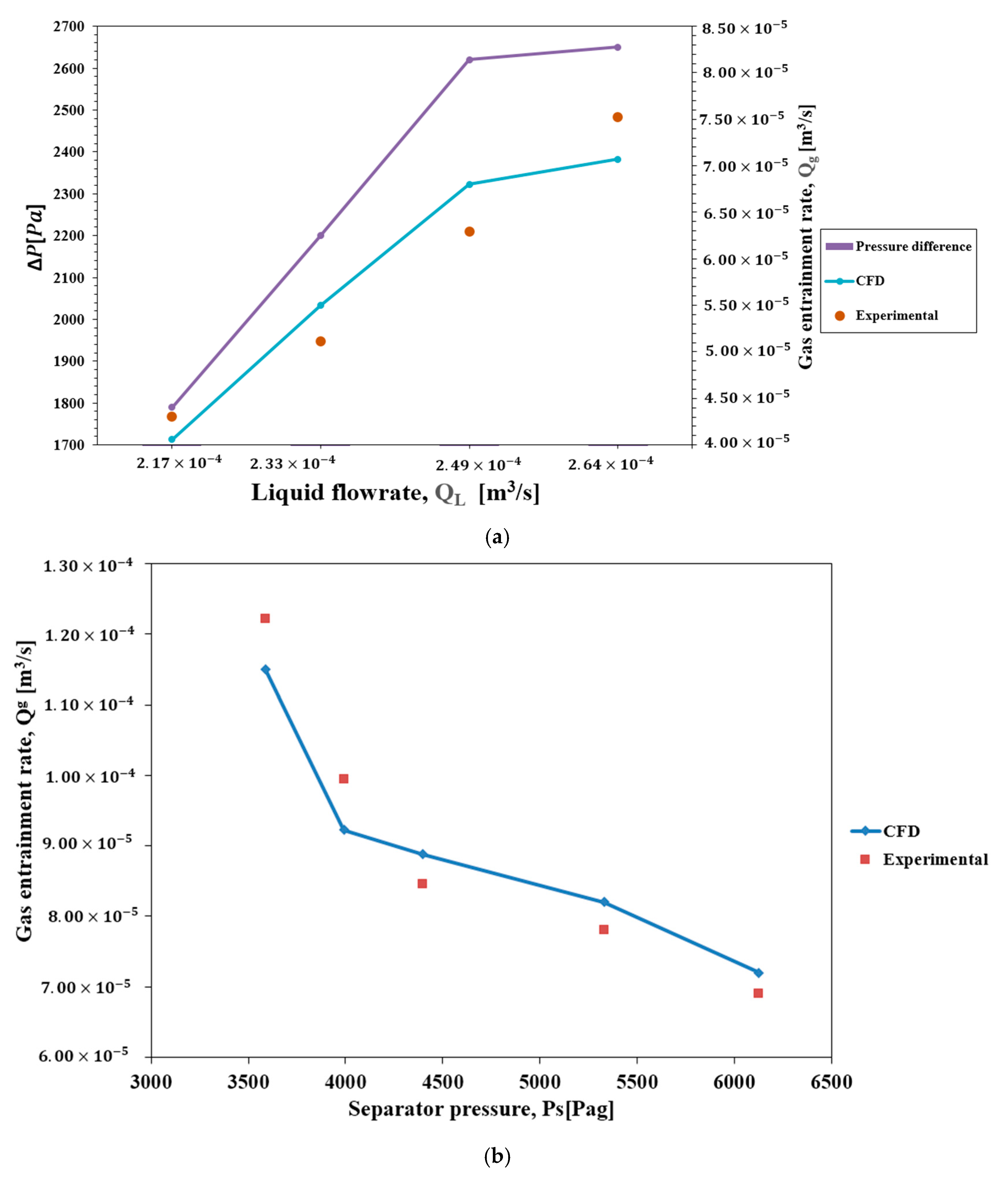
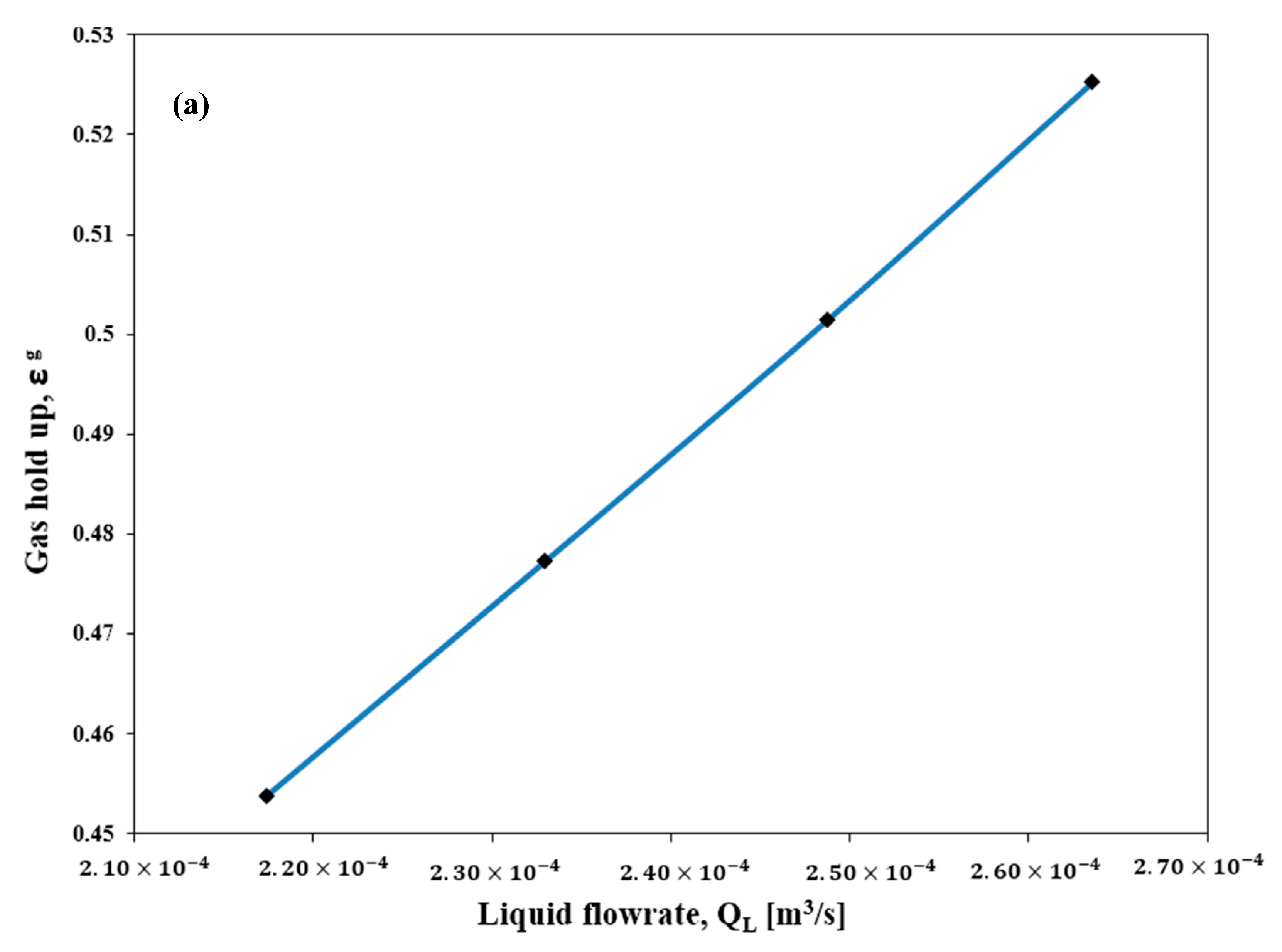
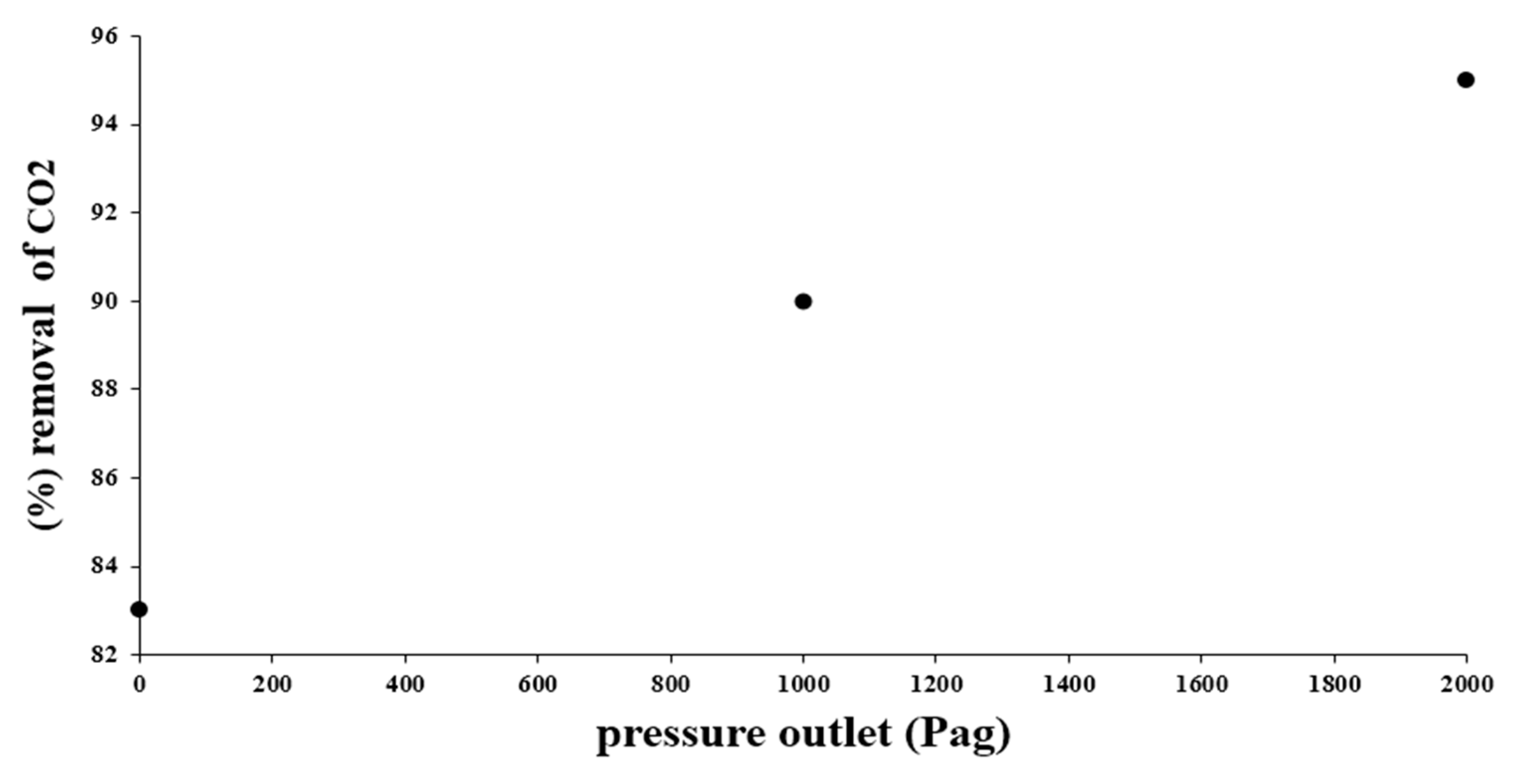
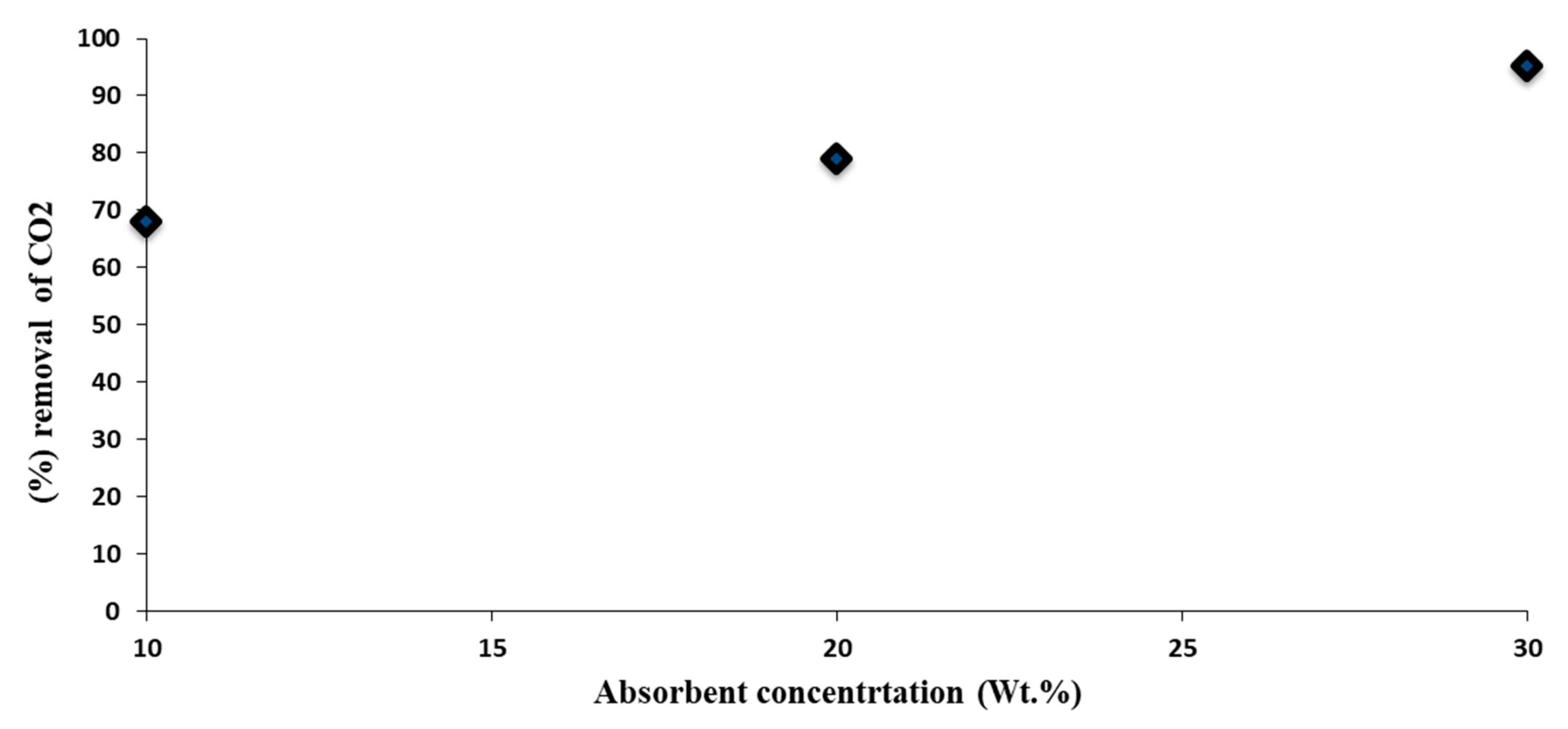
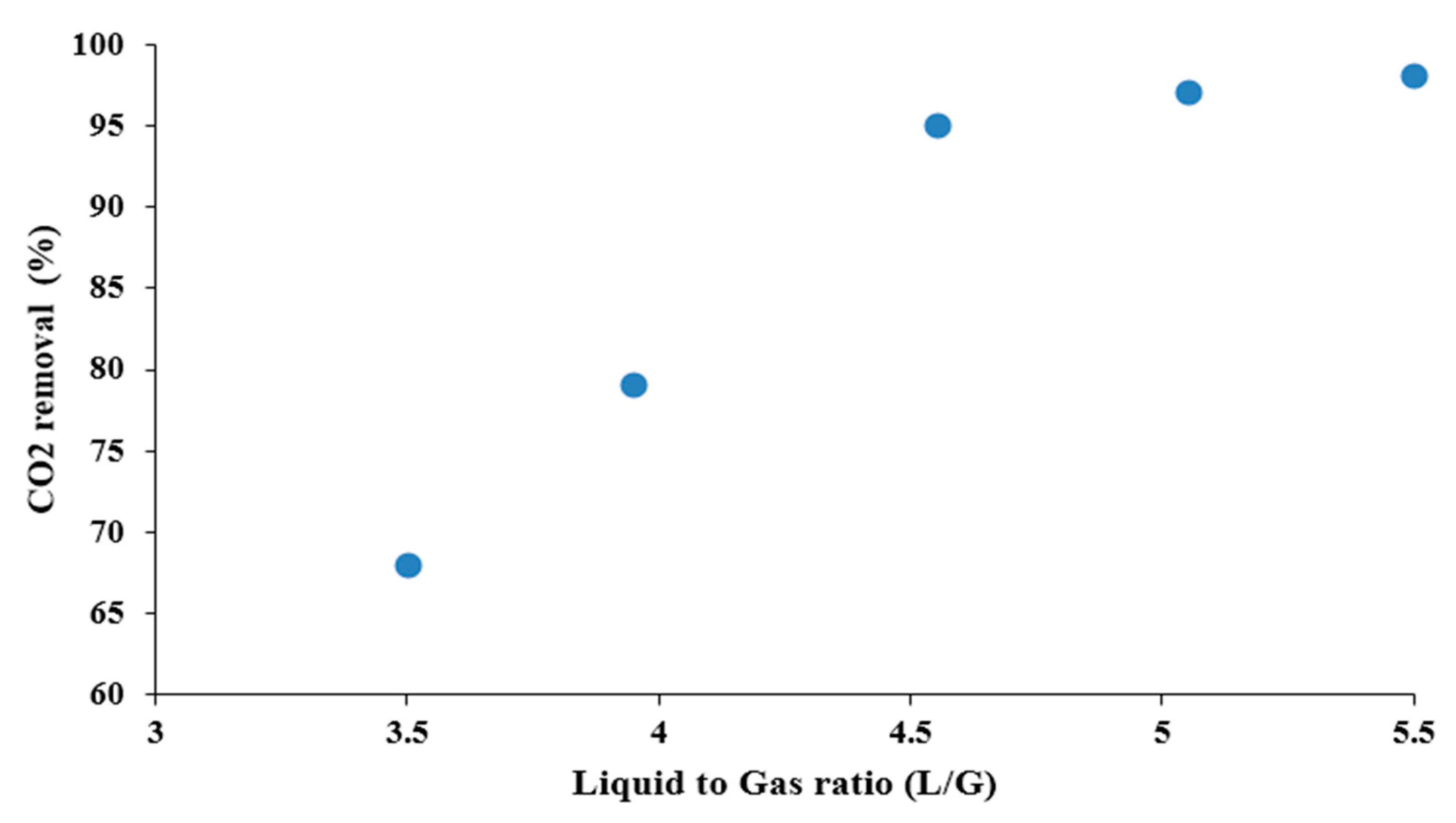
A CFD model is developed to illuminate the hydrodynamics and mass transfer characteristics of an ejector by employing the Eulerian–Eulerian multiphase fluid model and Standard k-$\epsilon$ model with 2D (air/CO₂-MEA solution) and 3D (air–water) modeling. For 3D geometry, the model was validated initially by altering the rate of liquid fluid flow in the range of 2.17 × 10⁻⁴ to 2.64 × 10⁻⁴ m³/s and outlet pressure in the range of 3000 to 6500 Pa, then the effects of these two parameters on gas phase hold-up, recirculation, the location of mixing shock, and negative pressure were investigated. Experimental data and CFD results are in good agreement. Mixing shock and position of its occurrence were investigated in this study as important factors. This three-dimensional phenomenon could be explained satisfactorily based on the results obtained from the 3D simulation. For 2D geometry and by considering the User-Defined Functions code, the effect of different parameters on CO₂ removal was considered. The following are the main findings: for the 3D ejector, it is found that with increasing the outlet pressure by about 70%, the rate of gas entrainment and gas hold up decrease by about 37% and 20%, respectively. The mentioned parameters showed increasing behavior of about 74% and 15%, respectively, when the mass flow rate of the liquid increased from 2.17 × 10⁻⁴ to 2.64 × 10⁻⁴ m³/s. It is observed that the location of mixing shock comes about at the end of the mixing tube. With an increasing mass flow rate of the liquid, the mixing shock is transferred from the ejector’s throat to the diffuser side. A greater negative pressure is observed when the mass flow rate of the liquid is increased. 2D ejector’s findings showed that %CO₂ removal is increased with increasing outlet pressure, absorbent concentration, and liquid-to-gas ratio.

References

1. Reis, L.B.; dos Santos Gioria, R. Optimization of liquid jet ejector geometry and its impact on flow fields. Appl. Therm. Eng. 2021, 194, 117132. [Google Scholar] [CrossRef]
2. Zolfaghari, M.; Pirouzfar, V.; Sakhaeinia, H. Technical characterization and economic evaluation of recovery of flare gas in various gas-processing plants. Energy 2017, 124, 481–491. [Google Scholar] [CrossRef]
3. Derthick, M. Statehouse and Greenhouse: The Emerging Politics of American Climate Change Policy; Brookings Institution Press: Washington, DC, USA, 2005. [Google Scholar]
4. Kadafa, A.A. Environmental impacts of oil exploration and exploitation in the Niger Delta of Nigeria. Glob. J. Sci. Front. Res. Environ. Earth Sci. 2012, 12, 19–28. [Google Scholar]
5. Rahimpour, M.; Asgari, A. Production of hydrogen from purge gases of ammonia plants in a catalytic hydrogen-permselective membrane reactor. Int. J. Hydrog. Energy 2009, 34, 5795–5802. [Google Scholar] [CrossRef]
6. Haidl, J.; Mařík, K.; Moucha, T.; Rejl, F.J.; Valenz, L.; Zednikova, M. Hydraulic characteristics of liquid–gas ejector pump with a coherent liquid jet. Chem. Eng. Res. Des. 2021, 168, 435–442. [Google Scholar] [CrossRef]
7. Wen, H.; Yan, J.; Li, X. Influence of liquid volume fraction on ejector performance: A numerical study. Appl. Therm. Eng. 2021, 190, 116845. [Google Scholar] [CrossRef]
8. Wang, X.; Li, H.; Dong, J.; Wu, J.; Tu, J.-Y. Numerical study on mixing flow behavior in gas-liquid ejector. Exp. Comput. Multiph. Flow 2021, 3, 108–112. [Google Scholar] [CrossRef]
9. Aidoun, Z.; Ameur, K.; Falsafioon, M.; Badache, M. Current advances in ejector modeling, experimentation and applications for refrigeration and heat pumps. Part 1: Single-phase ejectors. Inventions 2019, 4, 15. [Google Scholar]
10. Song, Y.; Ma, Y.; Wang, H.; Yin, X.; Cao, F. Review on the simulation models of the two-phase-ejector used in the transcritical carbon dioxide systems. Int. J. Refrig. 2020, 119, 434–447. [Google Scholar]
11. Bauzvand, A.; Tavousi, E.; Noghrehabadi, A.; Behbahani-Nejad, M. Study of a novel inlet geometry for ejectors. Int. J. Refrig. 2022, in press. [CrossRef]
12. El-Zahaby, A.; Hamed, M.H.; Omara, Z.; Eldesoukey, A. Study of the configuration and performance of air-air ejectors based on cfd simulation. ERJ. Eng. Res. J. 2015, 38, 15–30. [Google Scholar] [CrossRef]
13. Hosseinzadeh, M.; Ghaemi, A.; Shirvani, M. Hydrodynamic performance evaluation of a novel eductor liquid–liquid extractor using CFD modeling. Chem. Eng. Res. Des. 2017, 126, 19–31. [Google Scholar] [CrossRef]
14. Patel, D.; Chaudhari, A.; Laari, A.; Heiliö, M.; Hämäläinen, J.; Agrawal, K. Numerical simulation of bubble coalescence and break-up in multinozzle jet ejector. J. Appl. Math. 2016, 2016, 5238737. [Google Scholar] [CrossRef] [Green Version]
15. Aliyu, A.M.; Kim, Y.K.; Choi, S.H.; Ahn, J.H.; Kim, K.C. Development of a dual optical fiber probe for the hydrodynamic investigation of a horizontal annular drive gas/liquid ejector. Flow Meas. Instrum. 2017, 56, 45–55. [Google Scholar] [CrossRef]
16. Sharma, D.V.; Patwardhan, A.W.; Ranade, V.V. Estimation of gas induction in jet loop reactors: Influence of nozzle designs. Chem. Eng. Res. Des. 2017, 125, 24–34. [Google Scholar] [CrossRef] [Green Version]
17. Zheng, P.; Li, B.; Qin, J. CFD simulation of two-phase ejector performance influenced by different operation conditions. Energy 2018, 155, 1129–1145. [Google Scholar] [CrossRef]
18. Sharma, D.; Patwardhan, A.; Ranade, V. Effect of turbulent dispersion on hydrodynamic characteristics in a liquid jet ejector. Energy 2018, 164, 10–20. [Google Scholar] [CrossRef] [Green Version]
19. Reddick, C.; Sorin, M.; Sapoundjiev, H.; Aidoun, Z. Effect of a mixture of carbon dioxide and steam on ejector performance: An experimental parametric investigation. Exp. Therm. Fluid Sci. 2018, 92, 353–365. [Google Scholar] [CrossRef]
20. Mifsud, D.; Cao, Y.; Verdin, P.G.; Lao, L. The hydrodynamics of two-phase flows in the injection part of a conventional ejector. Int. J. Multiph. Flow 2019, 112, 219–242. [Google Scholar] [CrossRef] [Green Version]
21. Park, S.-K.; Yang, H.-C. An experimental investigation of the flow and mass transfer behavior in a vertical aeration process with orifice ejector. Energy 2018, 160, 954–964. [Google Scholar] [CrossRef]
22. Helios, M.P.; Asvapoositkul, W.; Kim, K.C. Experimental flow visualization and performance analysis of horizontal water-air ejector system. J. Sustain. Energy Environ. 2020, 11, 43–48. [Google Scholar]
23. Mandal, A. Characterization of gas-liquid parameters in a down-flow jet loop bubble column. Braz. J. Chem. Eng. 2010, 27, 253–264. [Google Scholar] [CrossRef]
24. Chiesa, M.; Mathiesen, V.; Melheim, J.A.; Halvorsen, B. Numerical simulation of particulate flow by the Eulerian–Lagrangian and the Eulerian–Eulerian approach with application to a fluidized bed. Comput. Chem. Eng. 2005, 29, 291–304. [Google Scholar] [CrossRef]
25. Fluent, A. Fluent 14.0 User’s Guide; ANSYS FLUENT Inc.: Canonsburg, PA, USA, 2011. [Google Scholar]
26. Versteeg, H.K.; Malalasekera, W. An Introduction to Computational Fluid Dynamics: The Finite Volume Method; Pearson Education: Prentice Hall, NJ, USA, 2007. [Google Scholar]
27. Frank, T.; Zwart, P.; Krepper, E.; Prasser, H.-M.; Lucas, D. Validation of CFD models for mono-and polydisperse air–water two-phase flows in pipes. Nucl. Eng. Des. 2008, 238, 647–659. [Google Scholar] [CrossRef]
28. Grace, J. Shapes and velocities of single drops and bubbles moving freely through immiscible liquids. Trans. Instn. Chem. Eng. 1976, 54, 167–174. [Google Scholar]
29. Auton, T. The lift force on a spherical body in a rotational flow. J. Fluid Mech. 1987, 183, 199–218. [Google Scholar] [CrossRef]
30. Drew, D.; Lahey, R., Jr. The virtual mass and lift force on a sphere in rotating and straining inviscid flow. Int. J. Multiph. Flow 1987, 13, 113–121. [Google Scholar] [CrossRef]
31. Tomiyama, A.; Tamai, H.; Zun, I.; Hosokawa, S. Transverse migration of single bubbles in simple shear flows. Chem. Eng. Sci. 2002, 57, 1849–1858. [Google Scholar] [CrossRef]
32. Wellek, R.; Agrawal, A.; Skelland, A. Shape of liquid drops moving in liquid media. AIChE J. 1966, 12, 854–862. [Google Scholar] [CrossRef]
33. Burns, A.D.; Frank, T.; Hamill, I.; Shi, J.-M. The Favre averaged drag model for turbulent dispersion in Eulerian multi-phase flows. In Proceedings of the 5th International Conference on Multiphase Flow (ICMF), Yokohama, Japan, 30 May–4 June 2004; pp. 1–17. [Google Scholar]
34. Antal, S.; Lahey, R., Jr.; Flaherty, J. Analysis of phase distribution in fully developed laminar bubbly two-phase flow. Int. J. Multiph. Flow 1991, 17, 635–652. [Google Scholar] [CrossRef]
35. Li, X.; Wang, W.; Zhang, P.; Li, J.; Chen, G. Interactions between gas–liquid mass transfer and bubble behaviours. R. Soc. Open Sci. 2019, 6, 190136. [Google Scholar] [CrossRef] [Green Version]
36. Zhang, D.; Deen, N.; Kuipers, J. Numerical modeling of hydrodynamics, mass transfer and chemical reaction in bubble Columns. In Proceedings of the 6th International Conference on Multiphase Flow (ICMF), Leipzig, Germany, 9–13 July 2007. [Google Scholar]
37. Penttilä, A.; Dell’Era, C.; Uusi-Kyyny, P.; Alopaeus, V. The Henry’s law constant of N2O and CO2 in aqueous binary and ternary amine solutions (MEA, DEA, DIPA, MDEA, and AMP). Fluid Phase Equilibria 2011, 311, 59–66. [Google Scholar] [CrossRef]
38. Mandal, B.P.; Kundu, M.; Bandyopadhyay, S.S. Physical solubility and diffusivity of N2O and CO2 into aqueous solutions of (2-amino-2-methyl-1-propanol+ monoethanolamine) and (N-methyldiethanolamine+ monoethanolamine). J. Chem. Eng. Data 2005, 50, 352–358. [Google Scholar] [CrossRef]
39. Maceiras, R.; Alvarez, E.; Cancela, M.A. Effect of temperature on carbon dioxide absorption in monoethanolamine solutions. Chem. Eng. J. 2008, 138, 295–300. [Google Scholar] [CrossRef]
40. Brauer, H. Particle/fluid transport processes. Prog. Chem. Eng. 1981, 19, 61–99. [Google Scholar]
41. Spalding, B. Turbulence models for CFD in the 21st century. In Proceedings of the ACFD 2000 Conferences, Beijing, China, 17–20 October 2000. [Google Scholar]
42. Majumder, S.K.; Kundu, G.; Mukherjee, D. Mixing mechanism in a modified co-current downflow bubble column. Chem. Eng. J. 2005, 112, 45–55. [Google Scholar] [CrossRef]
43. Cramers, P.; Beenackers, A. Influence of the ejector configuration, scale and the gas density on the mass transfer characteristics of gas–liquid ejectors. Chem. Eng. J. 2001, 82, 131–141. [Google Scholar] [CrossRef]
44. Kim, M.I.; Kim, O.S.; Lee, D.H.; Kim, S.D. Numerical and experimental investigations of gas–liquid dispersion in an ejector. Chem. Eng. Sci. 2007, 62, 7133–7139. [Google Scholar] [CrossRef]
45. Li, Z.; Yuan, Y.; Guo, B.; Varsegov, V.; Yao, J. The recirculation zone characteristics of the circular transverse jet in crossflow. Energies 2020, 13, 3224. [Google Scholar] [CrossRef]
46. Opletal, M.; Novotný, P.; Linek, V.; Moucha, T.; Kordač, M. Gas suction and mass transfer in gas-liquid up-flow ejector loop reactors. Effect of nozzle and ejector geometry. Chem. Eng. J. 2018, 353, 436–452. [Google Scholar] [CrossRef]
Figure 1. (a) The schematic of a flare gas recovery system, (b) the typical geometry of a liquid jet ejector.
Applsci 12 04485 g001
Figure 2. Schematic representation of inter-dependency of fluid flow, mass transfer, and chemical reaction.
Applsci 12 04485 g002
Figure 3. Dimensions, grid structures, and boundary conditions of 3D and 2D ejector.
Applsci 12 04485 g003
Figure 4. (a) Effect of motive liquid flow rate on the air entrainment (nozzle diameter = 6 mm) and pressure difference between the beginning and the end of the nozzle. (b) Effect of separator pressure on gas entrainment at constant liquid flow rate of 2.85 × 10⁻⁴ m3/s for the air–water system (nozzle diameter = 6 mm).
Applsci 12 04485 g004
Figure 5. (a) The effects of liquid flow rate (QL) on gas phase hold-up ( ε g ) for nozzle diameter = 6 mm and pressure outlet = 3250 Pag (b) The effects of separator pressure (Ps) on gas phase hold-up ( ε g ) at a constant liquid flow rate of 2.85 × 10⁻⁴ m3/s for the air–water system (nozzle diameter = 6 mm).
Applsci 12 04485 g005aApplsci 12 04485 g005b
Figure 6. Variation of gas phase hold-up with time at a constant liquid flow rate of 2.17 × 10⁻⁴ m3/s for the air–water system (nozzle diameter = 6 mm).
Applsci 12 04485 g006
Figure 7. (a) The pathlines of air velocity [m/s], (b) the vector of air velocity.
Applsci 12 04485 g007aApplsci 12 04485 g007b
Figure 8. Schematic of a circular transverse jet in cross flow [45].
Applsci 12 04485 g008
Figure 9. (a) The pressure contour [Pag], (b) the velocity contour [m/s].
Applsci 12 04485 g009
Figure 10. The effects of liquid flow rate on negative pressure, (a) flow rate: 2.49 × 10⁻⁴ m3/s, (b) flow rate: 2.64 × 10⁻⁴ m3/s.
Applsci 12 04485 g010
Figure 11. (a) The contour of volume fraction of the air in the ejector. (b) The plot of static pressure profile of ejector (along the center line of the ejector).
Applsci 12 04485 g011aApplsci 12 04485 g011b
Figure 12. The influence of the mass flow rate on the mixing shock phenomenon, (a) flow rate: 2.49 × 10⁻⁴ m3/s, (b) flow rate: 2.64 × 10⁻⁴ m3/s.
Applsci 12 04485 g012
Figure 13. UDF flow chart for the m ˙ G L maximization.
Applsci 12 04485 g013
Figure 14. Impacts of ejector outlet pressure on removal of CO2 (dnozzle = 6 mm-QL = 2.85 × 10⁻⁴ m3/s, [MEA] = 30%Wt).
Applsci 12 04485 g014
Figure 15. Ejector segmentation to calculate the average mass fraction in each part.
Applsci 12 04485 g015
Figure 16. The mass fraction contour of CO2 in the gas phase along the ejector for (a) 0 Pag output pressure and (b) 2000 Pag output pressure.
Applsci 12 04485 g016
Figure 17. Impacts of absorber’s concentration on the amount of CO2 removal (dnozzle = 6 mm-QL = 2.85 × 10⁻⁴ m3/s, pressure outlet = 2000 Pag).
Applsci 12 04485 g017
Figure 18. Effect of the liquid-to-gas (L/G) ratio on the percentage of CO2 removal.
Applsci 12 04485 g018