Mode Choice Effects on Bike Sharing Systems

Abstract

Bike-sharing systems (BSS) are offered in many cities and urban municipalities and urban areas without such systems are thinking about their introduction. In addition, many studies on BSS are available; however, neither mode nor route choice parameters are available for station-based BSS, which are required for the implementation of BSS in local and regional transport demand models. As a result, this makes it impossible to simulate demand model-based effects of these systems on other transport modes and e.g., calculate scenario-guided modal shifts. The paper presents results obtained from a survey study, which aims to estimate BSS-related choice parameters. The study combined computer-assisted telephone interviews (CATI) for a collection of revealed preferences (RP) on the use of BSS with a follow-up paper-and-pencil survey on stated preferences (SP) of 220 BSS users and non-users from the Rhine-Neckar area in mid-west Germany. Considering the three transport modes BSS, public transport (PT), and private motorized transport (PMT), results from this choice experiment and, according to behavioural parameters, allow integration of BSS in transport demand models and a simulation of modal shifts. Survey design, mode-choice experiment, and choice models are presented in this paper.

1. Introduction

The first bike-sharing systems (BSS) were introduced around five decades ago. Over the past two to three decades, the number of BSS has increased, and such systems are nowadays available in many cities around the globe. It is, however, surprising, that parameters for neither BSS-related mode nor route choices are currently available. This results in a lack of knowledge of behavioural patterns. Amongst other purposes, such parameters are needed for the implementation of BSS as a transport mode in transport demand models and to calculate, e.g., modal shifts.

To estimate such parameters, a survey study was conducted in the field in Germany and collected information on mode- and route choices from around 220 participants in an existing station-based BSS. This BSS was introduced in 2012, and is located in the Rhine-Neckar area in mid-west Germany, including 20 municipalities in total; 4 of them are major cities (Mannheim, Ludwigshafen, Heidelberg, Kaiserslautern), 11 are mid-size municipalities and 5 are smaller towns. The survey study combined computer-assisted telephone interviews (CATI) for a collection of revealed preferences (RP) on the use of BSS with a follow-up paper-and-pencil survey on stated preferences (SP) for BSS users and non-users. The choice experiment considers the three transport modes: BSS, PT, and PMT.

This effort resulted in a rich data set, which allows an analysis of behavioural patterns in terms of BSS-related mode and route choices and a quantification of the needed parameters; with that, the study closes a knowledge gap and allows the implementation of station-based BSS in local or regional transport demand models and according to simulations with these tools.

The paper focuses on mode choices exclusively. Section 2 presents results from literature analysis and aims to identify attributes of relevance for choices pro or against BSS-use. Section 3 introduces the study area and an existing BSS, that was used to recruit survey participants and collect information on BSS use. Furthermore, the recruitment strategy, survey protocol, and experimental design for the choice experiment are presented. Next, descriptive statistics on respondents’ socio-demographics and their choices are provided in Section 4 together with the model formulation. Section 5 presents results on model development and the final multinomial logit models on choices between the alternatives BSS, public transport (PT), and private motorized transport (PMT). The models are estimated for mandatory and leisure trips and model results are accompanied by interpretations. Finally, conclusions and an outlook on future research are drawn in Section 6.

2. Literature Review

BSS were introduced in many cities around the globe in the last decade. In parallel, the number of studies on BSS has increased as well (for comparative meta-studies see e.g., Refs. [1,2,3,4,5]). Most of these studies indicate that BSS-use substitutes sustainable modes such as walking and PT; however, some report that BSS-use also reduces trips by car and other PMT means. The effect on PMT is closely related to the synergetic effects of multi- and intermodal combinations of BSS with PT and promoting cycling in general [5]. In order to incorporate BSS into transport demand models and thus estimate more comprehensively the potential of reducing car trips, it is necessary to understand the mode and route choice behaviour of (potential) BSS users; so far, only a few studies focused on mode and route choice behaviour of BSS-users see Refs. [6,7,8,9], while much more studies exist for cycling with private bikes. Filling this gap is the aim of the survey, which is presented in the following sections.

Several research studies investigated the influence of different attributes on cycling. Buehler and Dill [10] reviewed the effects of cycling infrastructure; among other things, they found that cyclists tend to prefer separated bike lanes, lower speed limits and volumes of motorized traffic, trees along the route, and routes with fewer intersections; further, they tend to avoid routes with on-street parking and many variations in altitude.

Other studies investigated the effects of the built environment to enhance walking and cycling levels [11,12]. Their main findings highlight the importance of short distances to destinations, mixed land use with high densities of population and facilities for groceries, retail, service, and recreation), charges for car parking, and a network of convenient cycling infrastructure for increased shares of bike-use. What cyclists perceive as convenient highly depends on the study location, but amongst other factors, they prefer segregation or protection from motor traffic, little or only small detours, avoidance of intersections with motor traffic, and bike parking facilities.

Studies have also investigated how the built environment affects the use of bike-sharing stations [13,14]. It was found that high densities and proximity to cycling-friendly routes and to PT stations play a crucial role; furthermore, a study from Lisbon described an algorithm-based approach for the identification of optimal locations for stations and fleet dimensions for BSS by taking into account user demand, renting-costs, and a mixed fleet of regular and electric bikes [15].

In addition, there are studies, which explicitly investigated the mode choice behaviour of cyclists on both private and shared bikes: Hamre and Buehler [16] studied the mode choice behaviour of around 4.600 commuters in Washington; their result is those bike parking facilities, non-free car parking, and showers at work increase the utility of commuting by bike. In another study, cycling was compared with bus riding and driving with respect to travel time reliability [17]; it was found that for habitually repeated trips, travellers rate reliability higher than travel time. Campbell et al. [6] investigated the factors influencing the choices for bike-sharing (conventional bike and e-bike) in Beijing [6]; they found that trip distance, rain, temperature, and poor air quality negatively impact the choice for non-electric BSS on the one side. On the other side, they reported that users’ socio-demographic characteristics only play a minor role. A study from Switzerland [18,19] compared several mode-specific effects on choices between PMT, PT, cycling, and walking under the inclusion of individuals’ and area-specific characteristics, whereby for walking and cycling only the effect of travel time was considered as a mode-specific attribute; they found that car availability, younger age, low fuel, and parking costs, and low parking search times increase the utility of PMT, while low access and egress times, low ticket costs, and a low utilized capacity increase the utility of PT. An investigation on the Dutch mobility panel with almost 2000 participants focused on characteristics that affect choices between PMT, PT, cycling, and walking [20]. Among others, these characteristics include individual and household characteristics (such as socio-demographics and mobility ownership), weather, trip characteristics (such as distance and travel time), effects from the built environment, and work characteristics. Results indicate that, among other things, higher education, transit subscription, cycling to high school, weekdays, and certain trip purposes increase the utility of cycling, while owning a company car and travelling in larger groups decrease its utility. A recent study compared shared modes in Zurich, namely station-based BSS, e-bike sharing systems (e-BSS), and e-scooters [7]; they found that station density and morning hours increased the utility of BSS, while variation in topographical altitude and night hours decreased its utility. Ilahi et al., (2021) undertook an extensive survey with more than 5000 participants from the Greater Jakarta area in which they also incorporated less-established modes such as urban air mobility, including currently developed electric-based aircraft or autonomous vertical take-off and landing vehicles, on-demand transport, and bus rapid transit [21]; they found that motorcycles have the highest baseline utility, while bikes have the second-lowest.

In addition, numerous studies have focused on the route choices of cyclists. Although this paper is primarily focused on mode choices, it can be expected that route choice effects in general also affect mode choices. A recent study with 662 participants from Greece and Germany investigated the effects of cycling infrastructure, speed limit, surface, on-street parking, trees, and travel time on route choices [22]; they found that in both countries protected bike lanes are preferred over other forms of infrastructure. Furthermore, asphalt is preferred over cobblestone, while the utility of a speed limit depends on the country. Other attributes that were incorporated in older studies are the number of car lanes [23], stop signs and crowding of cyclists [24], number and type of crossings [25], the width of bike lanes and traffic volumes [26], as well as sharing space with pedestrians and the availability of secure parking and showers at the destination [27].

With reference to the presented studies, it can be assumed that relevant attributes for cycling with private bikes are relevant for BSS, too. Furthermore, additional attributes, such as renting costs, access and egress times, to renting stations are relevant in the case of BSS. Evaluating which effects are of relevance for BSS and quantifying their influence is the aim of our survey study. The employed survey design and choice experiment are introduced in the following section. The study aims to provide an overview of the most relevant effects to allow the implementation of BSS in multi-modal transport demand models, and, with that, to provide a basis for forecasts on urban transport, which consider BSS as an alternative transport mode.

3. Survey Design and Choice Experiment

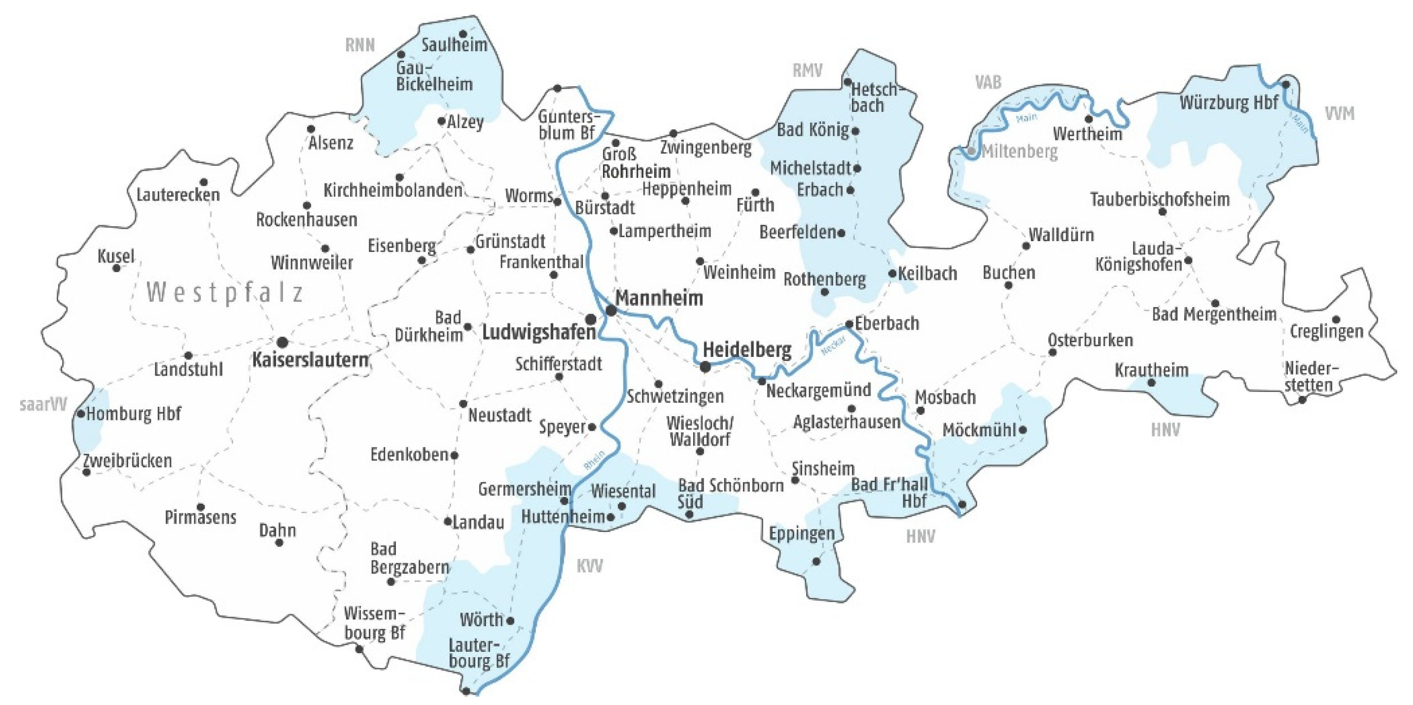
In 2020, the transport association Rhine-Neckar (VRN) decided to evaluate the performance of its BSS named VRNnextbike and especially focus on users and their behavioural patterns such as e.g., origins and destinations of rental bike trips, trip purposes, average renting times, and distances. Figure 1 provides an overview of the supply area of VRNnextbike, which lies in Mid-West Germany; it includes 20 municipalities in total; 4 of these municipalities are major cities (Mannheim, Ludwigshafen, Heidelberg, Kaiserslautern), 16 are minor cities with 11 mid-size municipalities and 5 smaller towns.

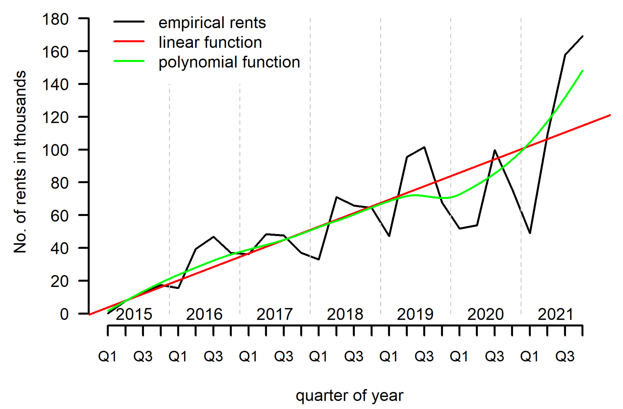
Figure 2 provides an overview of the absolute development of bike rents between 2015 and 2020; it documents a positive development trend and repeating temporal patterns between annual seasons. Furthermore, it shows the effect of the first Corona-Lockdown in the second quarter of 2020 and the quick recovery of the system in the third quarter.

Evaluating the BSS VRNnextbike and analyzing user behaviour in terms of, e.g., socio-demographics made it necessary to design a survey study. This provided the opportunity to include items on the effects of mode and route choices in terms of a BSS and to quantify mode and route choice parameters. Collecting data on BSS-related mode and route choices; however, made it necessary to extend the survey framework and include a stated choice experiment. In addition, the target population had to be extended. While the VRN-survey wanted to focus on BSS users exclusively, the choice experiment made it necessary to include non-users as well, to understand differences in the perception between these two groups and allow a later simulation of, e.g., modal shifts. For this reason, a hybrid recruitment strategy and a specific survey protocol for BSS users on the one side and non-users on the other side were employed and a stated preference experiment was developed and included in the survey.

The following descriptions and data analyses focus on the mode choice experiment exclusively. The route choice experiment and recording results will be presented in the future. Readers who are interested in the results are encouraged to contact the research team.

3.1. Recruitment Strategy

Table 1. Frame population and recruitment strategy.

	Subsample 1: BSS-Users	Subsample 2: BSS Non-User
Frame-population	Users of BSS VRNnextbike	BSS non-user residents from VRNnextbike supply area
Recruitment	Via the nextbike app at the start or end of bike-rent	Recruitment call via telephone
Survey mode	Computer-assisted telephone interviews (CATI) and paper-and-pencil questionnaire with a postpaid return envelope	Paper-and-pencil questionnaire with a postpaid return envelope
Incentive	EUR 20 after participation in the CATI and again after returning the filled-out questionnaire	EUR 20 after returning the filled-out questionnaire

presents an overview of the frame population and recruitment strategy of the survey study, which was split and specifically designed for BSS users and non-users. BSS users, on the one side, were recruited electronically either before or after renting a bike from VRNnextbike. During the electronic check-in or -out of the rented bike in the VRNnextbike smartphone app, they have presented an invitation to participate in a computer-assisted telephone interview (CATI) on their travel behaviour, bike-rent habits, and the BSS-trip they performed either before or after the recruitment. To participate, they were asked to mention their preferred daytime for a 30-min telephone interview within the next week and, in addition, to report their age, gender, and city of residence in an electronic recruitment questionnaire. Questions on socio-demographics aimed to keep control over the distribution of socio-demographic characteristics in the CATI sample. Participation in the electronic recruitment questionnaire took about two minutes on a smartphone. Accompanying the questions, information on data protection and the aim of the research project was provided on linked websites and an incentive of EUR 20 for participation in the CATI was mentioned. After participants completed the CATI, they were recruited for the subsequent paper-and-pencil questionnaire, which was sent via postal mail to the respondents. Enhancing convenient participation was the aim of this study, ensured by sending an addressed and postpaid mail-back envelope together with the questionnaire, including additional information on the study and data protection.

BSS non-users, on the other side, were recruited from a sample of randomly generated phone numbers for the supply area of VRNnextbike. These phone numbers might in some cases have resulted in interviews with BSS-users; however, this approach was chosen as only 2.9% of all inhabitants in the supply area are BSS-users and sampling a user of VRNnextbike was for this reason rather unlikely; furthermore, a control questions whether respondents are BSS users was added to allow the identification in the analysis. Recruitment of this subsample was done via telephone by asking for gender, age, and city of residence to keep control over the distribution of socio-demographic characteristics. In addition, the telephone recruitment aimed to provide information on the study, and data protection issues and to discuss potential respondents´ questions. In addition, an incentive of EUR 20 was offered for a filled-out survey instrument. Like in the sample for BSS users, the printed paper-and-pencil questionnaire was sent via postal mail to the respondents, which included an addressed and postpaid mail-back envelope.

3.2. Revealed and Stated Preferences: Survey Protocol

Choices on, e.g., transport modes and routes can be observed either in real-life situations or in hypothetical choice situations. Real-life observations result in information on revealed preferences (RP) whereas observations of hypothetical choices result in data on stated preferences (SP). RP data have the advantage of representing peoples´ actual behaviour; they, however, also include disadvantages such as little variation in attributes, which could be used to explain choices (e.g., travel times by bus on a specific route), and issues of multicollinearity (e.g., travel times, distances, and costs are often highly correlated for a specific transport mean). In addition, future effects, demands, and supplies cannot be addressed with RP data. SP and according to hypothetical choices overcome these issues. Here, an experimental design is employed, that focuses on selected and potentially future attributes. It asks respondents to exclusively consider these selected effects when making their choices. Attribute variation is controlled by an experimental design, which allows overcoming the challenge of multicollinearity. The disadvantages are, however, the hypothetical character of the choice tasks and the reduction of complexity (for a more detailed discussion on RP- and SP choices see, e.g., Refs. [19,28,29]).

In transport planning, RP and SP data are often combined to overcome the mentioned limitations of the SP approach. One way to increase the reliability of SP choices is to employ an individual´s RP decisions as the basis for her or his SP-choice situations [30] (for a discussion of combined RP–SP studies see Ref. [19]). This means, on the one hand, an increased complexity for the fieldwork, as choice situations are individually tailored for each participant of the SP survey. On the other hand, the RP–SP combination increases the quality of a survey as the choice situations are based on former choices of a respondent, transport familiarity and thus allow an easy imagination of the choice situation under observation. The more realistic and familiar a choice situation is, the less effort it takes to be contextualized resulting in more reliable respondents’ answers (for choice situations see Ref. [31]; for a more general discussion on response burden see Ref. [32])

In the CATI for BSS-users, information on mobility-tool ownership, trip characteristics of the BSS-use at the time of recruitment, attitudes on BSS, and socio-demographics were collected. During the interview, the chosen route of the rental bike trip was traced electronically by employing an online routing tool [33] to gather additional information for the trip, such as travel time and road surface. The collected information and RP data were employed as a basis for the mode choice experiment. Based on these BSS attributes, trip characteristics for the alternative modes PT and PMT were collected using an online routing provider [34] and an electronic PT-schedule service [35]. The choice experiment itself was designed as a follow-up survey and presented to those CATI participants, who agreed in filling out the paper-and-pencil questionnaire.

As RP data were not available for BSS non-users, aggregated RP characteristics on BSS usage were employed as the basis for the SP experiment. The aggregated figures for travel time were calculated on the automatically recorded data from the BSS VRNnextbike by discriminating between short, middle, and long trips for both major and minor cities (on average trips of the length of 0.8, 1.5, and 3.2 km for major cities, and 0.7, 1.4, and 4.4 km for minor cities), while averages for access and egress times were obtained from the BSS user-survey. In this case, data on mode alternatives were based on aggregated figures from the national travel survey in Germany [36], taking into account differences between major and minor cities. To design an individual questionnaire for this subsample, firstly, each respondent was assigned to a town size group based on his or her postal address. Secondly, every participant was sequentially assigned to a short, middle, or long trip distance and a trip purpose, either a leisure or mandatory activity at the trip destination. The resulting RP-values for each BSS non-user were employed as the basis for SP-experiment and its variations of attributes.

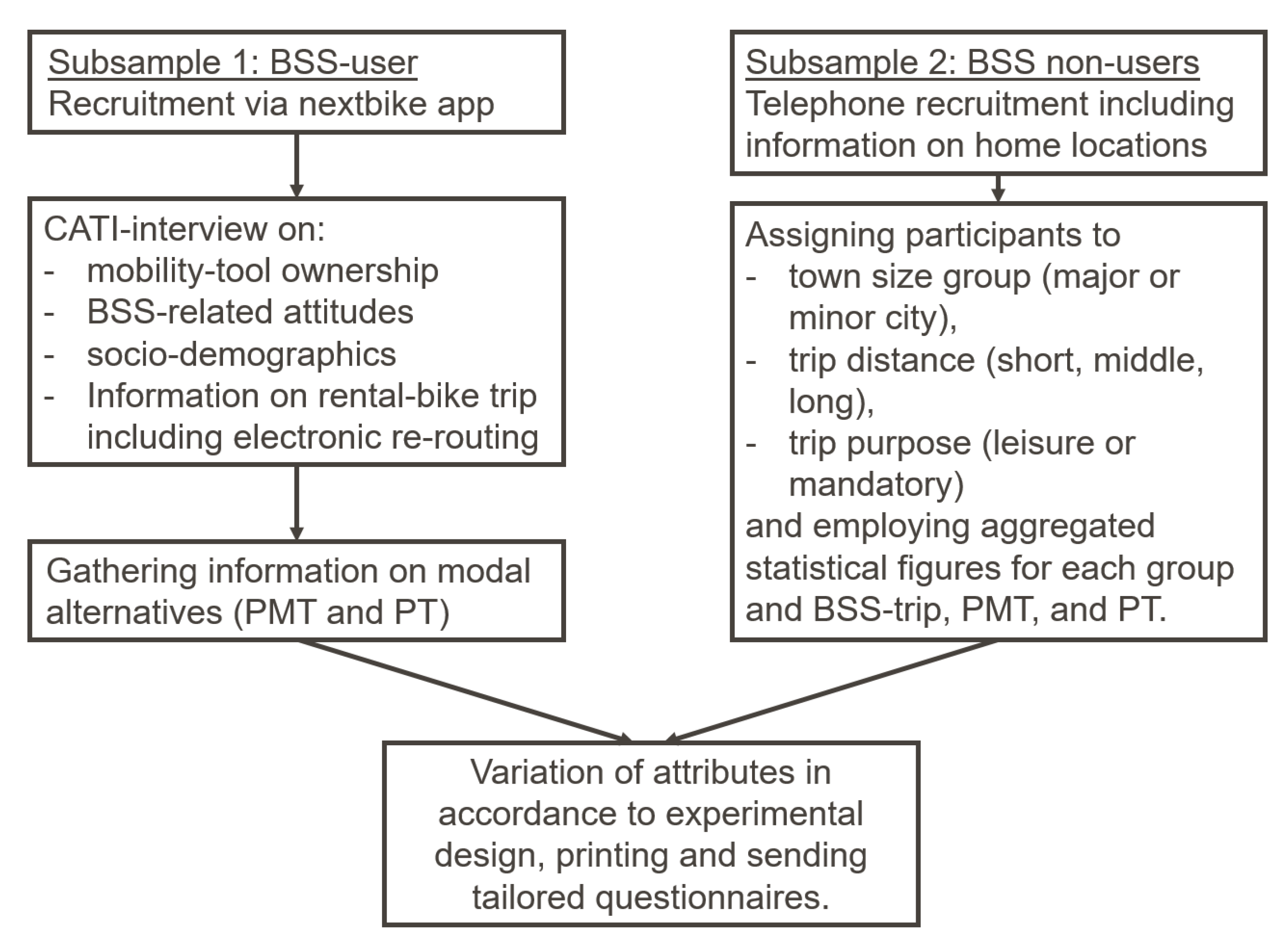
The recruitment procedure of both subsamples is visualized in Figure 3.

3.3. Experimental Design and Choice Situations

Attributes of the mode choice experiment were taken from former studies on mode choices and studies on selected transport modes such as bikes, PMT, and PT (see Literature Review in Section 2). Furthermore, they were discussed with external academic partners and practitioners from transport planning offices.

As described above, RP information (for BSS users) or aggregated empirical figures (for BSS-non-users) were employed and empirical values for the alternative modes were collected. Next, an individually tailored SP questionnaire was created by varying the mode-specific characteristics in accordance with a predefined experimental design. An overview of the attributes and variation of attribute levels is provided in

Table 2. Stated preference experiment: transport modes, attributes and variation.

Mode	Attribute	Variation of Reference Values/Levels
BSS	access and egress time	−50%/−10%/+40%
	travel time (TT)	−30%/−10%/+30%
	travel costs	−100%/−35%/+20%
	street type	cycleway/side street/arterial road
	surface type	asphalt/cobblestones/macadam
PMT	travel time (TT) incl. parking search	−20%/−10%/+30%
	fuel costs	−50%/+150%/+200%
	parking costs	−50%/+100%/+200%
PT	access and egress time	−50%/−10%/+40%
	travel time (TT)	−30%/−10%/+30%
	travel costs	−100%/−35%/+20%
	utilized capacity	middle/high/overloaded

.

To reduce the number of possible combinations of the presented variation levels, an efficient design [37] was generated with the software Ngene [38]; it resulted in 60 combinations to design the choice tasks, which were split into six blocks (the experimental design is available upon request). Each participant was assigned to one block and the empirical values were varied accordingly. Finally, each participant was asked to complete ten choice tasks in the paper-and-pencil questionnaire. Participation in the study was restricted to adults (18 years and older) owning a driver’s license to make the alternative PMT realistic.

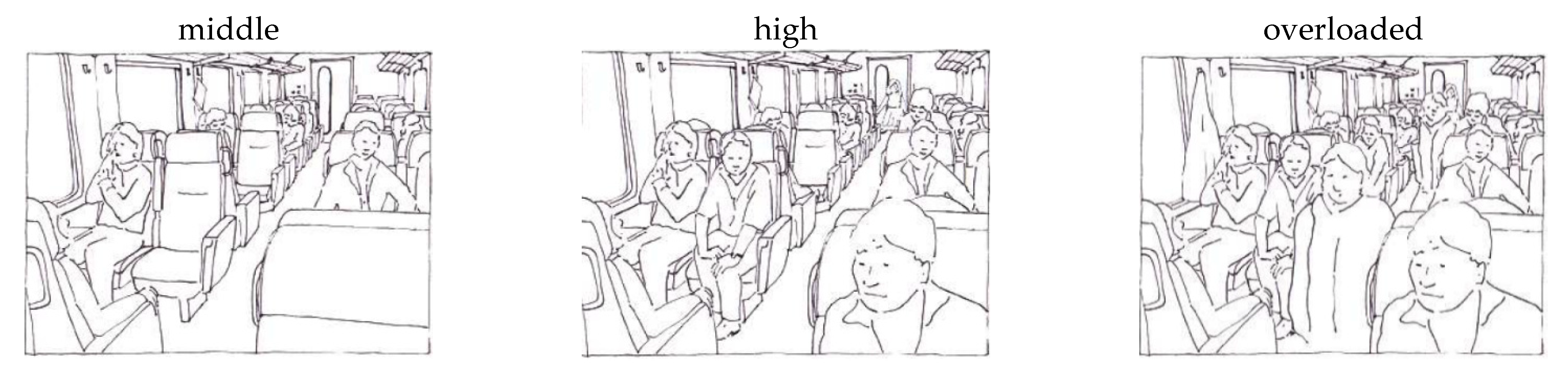
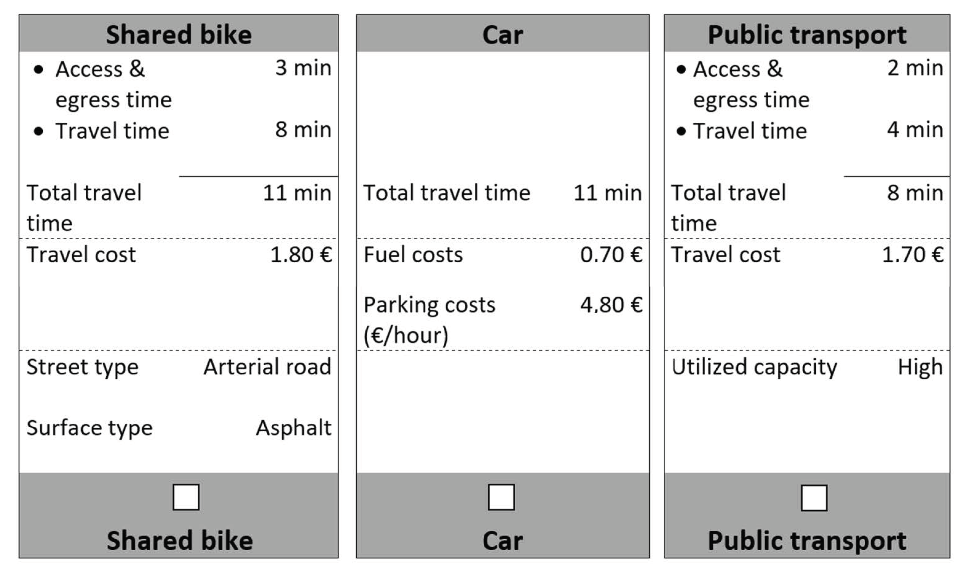
The individually tailored paper-and-pencil questionnaires were created, printed and sent within one week after recruitment to avoid fatigue effects. To increase reliability in terms of PT utilized capacity, an illustration accompanied the questionnaire (see Figure 4; for more details on reliability see Ref. [19]).

Both the survey protocol and instrument followed the suggestions by Dillmann [39]. After four weeks of non-response, reminders were sent with a new copy of the questionnaire. An exemplary choice situation is shown in Figure 5.

4. Descriptive Statistics and Modelling Approach

The survey was in the field from September 2021 to February 2022. After data cleaning, information from 220 respondents, who filled out and returned the questionnaire, was collected. On average, respondents answered 9.93 (median = 10) mode choice tasks, which resulted in a total of 2184 observations for the analysis. 27 respondents (12.3%) showed non-trading behaviour, meaning they chose an identical transport mode in all presented choice tasks.

4.1. Descriptive Statistics

Respondents from the subsample recruited via randomly generated phone numbers (see subsample 2 in

Table 3. Relative frequency distribution of selected sample characteristics.

Character	BSS-Users	BSS Non-User	Whole Sample
Sample size	128 (58%)	92 (42%)	220
Gender
Male	64.1%	41.3%	54.5%
Female	35.9%	58.7%	45.5%
Age
18–30 yr	71.1%	14.1%	47.3%
31–65 yr	28.9%	59.8%	41.8%
66–94 yr	0%	26.1%	10.9%
Home Municipality
City	89.1%	64.1%	78.6%
Larger town	9.4%	25.0%	15.9%
Smaller town	1.6%	10.9%	5.5%
Chosen alternative
BSS	760 (59.6%)	373 (41.1%)	1133 (51.9%)
PMT	111 (8.7%)	333 (36.7%)	444 (20.3%)
PT	405 (31.7%)	202 (22.2%)	607 (27.8%)

), who indicated to use a BSS, are considered BSS-users in the following analytical procedure (n = 11). Information on the distribution of selected socio-demographic characteristics and the frequency of chosen transport modes in the choice experiment for both subsamples and the whole sample are presented in Table 3.

Around 58% of all participants were BSS users and 42% are non-users. Users were more often males (64.1%) than non-users (41.3%). For the whole sample, the gender proportion was more balanced with 54.5% males and 45.5% females. BSS users belonged remarkably more often to younger age groups than non-users. Again, the proportion between young adults (18–30 years; 47.3%) and middle-aged persons (31–65 years; 41.8%) was more balanced for the whole sample. There are only a few observations of people in the retired age group (66–94 years): 0% for BSS-users, 26% for non-users and around 11% for the whole sample. Furthermore, around 89% of the user-sample lives in cities, 9% in larger towns and around 2% in small municipalities. This fits well with the automatically tracked renting numbers of VRNnextbike [40]. The non-user sample includes more respondents from larger towns (25%) and small municipalities (around 11%). In summary, there is socio-demographic variation in the data, and it can be assumed that evaluations from people with different socio-demographic characteristics are considered in the analysis.

Concerning mode choice situations, respondents from the user sample most often chose the BSS (around 60%), followed by PT (around 32%) and PMT (9%). Non-users also preferred the BSS (64%), however, followed by PMT (37%) and PT (22%).

Covariates in the behavioural experiment are based on RP-data for subsample 1, respondents recruited during the CATI, and on aggregated empirical figures for subsample 2, respondents recruited from the random phone number sample.

Table 4. Empirical distribution of covariates in a choice experiment.

Mode	Attribute	min	1st Qu.	Median	Mean	3.rd Qu.	Max
BSS	access and egress time [min]	1.0	4.0	6.0	6.3	10.0	49.0
	travel time [min]	1.0	6.0	10.0	12.4	15.0	108.0
	travel costs [EUR]	0.0	0.0	1.0	1.2	1.8	10.8
PMT	travel time incl. parking [min]	6.0	12.0	15.0	15.8	19.0	46.0
	fuel costs [EUR]	0.1	0.2	0.6	0.7	1.2	6.2
	parking costs [EUR]	0.6	0.8	3.2	2.7	3.3	4.8
PT	access and egress time [min]	0.0	4.0	6.0	7.0	9.0	41.0
	travel time [min]	1.0	6.0	9.0	10.5	14.0	64.0
	travel costs [EUR]	0.0	0.0	1.8	1.8	2.9	7.3

presents the empirical distribution of these covariates as included in the experiment.

In terms of the BSS, access and egress time has a minimum of 1 min, a median of 6 min, a mean of around 6 min and a maximum of 49 min. This distribution is comparable to access and egress for PT. BSS trips are short with a median travel time of 10 min and 15 min for the 3rd quartile. A few trips, however, are long with a maximum of 108 min. Travel costs are low, with EUR 1.80 for the 3rd quartile.

The overall travel time (including parking search time) of PMT is substantially higher than the travel time for BSS and PT. The minimum travel time is 6 min, 1st quartile at 12 min, median at 15 and 3rd quartile at 19 min. The maximum travel time, however, is 46 min and substantially lower than the maximum travel times for BSS and PT. Fuel costs for the trip show a range between EUR 0.10 for a very short trip and EUR 6.20. Parking costs lay between EUR 0.60 and EUR 4.80 with a median of EUR 3.20.

Access and egress times and travel times for PT are overall comparable to BSS. In terms of travel costs, PT shows moderate values between BSS and PMT.

4.2. Model Formulation

Discrete choice data, where respondents choose between a limited number of alternatives, are commonly analyzed by applying random utility maximization theory. The theory assumes rational behaviour in which respondents choose the alternative with the highest utility [29,41,42,43]. Namely, an individual $n$ faced with $J$ alternatives in $T$ choice tasks associates an indirect utility $U_{njt}$ for an alternative j in a choice task t and chooses the alternative with the highest utility. The utility of an alternative j is therefore decomposed as

$$U_{njt}=V_{njt}+{\epsilon }_{njt}={x^{\prime }}_{njt}\beta +{\epsilon }_{njt}$$

(1)

where $U_{njt}$ is not observed, but $V_{njt}$ is the deterministic utility of alternative $j$, and ${\epsilon }_{njt}$ is a random component not included in $V_{njt}$. The deterministic utility $V_{njt}$ can be specified by the term ${x^{\prime }}_{njt}$, where $x$ is a vector of explanatory variables (e.g., attribute levels), and $\beta$ is the corresponding coefficients to be estimated.

For each alternative, a utility function ($V_{njt})$ is specified, whereby the alternative-specific attributes, characteristics of the respondent or the choice situation are included as explanatory variables. When specifying the utility function, it is important to understand that only the differences in utility matter, while the scale of utility is arbitrary [29] (p. 19). Therefore, to capture the differences in the utility of the alternatives, $J\text{-}1$ alternative-specific constants (ASC) are specified, whereby the estimated ASCs are interpreted relative to the omitted alternative, which is normalized to zero [29,43]. For the categorical attributes, street type, surface type, and utilized capacity, the $L$ levels of each attribute were transformed into $L-1$ dummy variables. This means, the utility for one level per attribute is normalized to zero and serves as a reference category, while the parameter estimates for the $L-1$ dummy variables capture the utility differences to this reference category [28,29,43].

5. Results

The 2184 observations (choice tasks) were analyzed by estimating multinomial logit models (MNL) [44] in R [45,46], whereby BSS was chosen as reference alternative when specifying the equations for estimation. Firstly, an initial MNL was estimated by including exclusively effects of attributes from the choice experiment (see Table 2; for a documentation of this work see Ref. [47]). With reference to previous studies on mode choice [18,19,20,21] effects of socio-demographics (age, gender, education, student status, car availability, PT season ticket availability), home municipality, and season (winter vs. autumn) were expected. Consequently, as recommended in methodological literature [29,44] the initial model was sequentially built up by including these effects as alternative-specific attributes in maximum J-1 alternatives (one alternative as reference category), testing the hypotheses, and comparing the models (restricted vs. unrestricted) to omit parameters without significant effects and/or substantial improvement in the model fit. Further, it was assumed that the effects of travel time and travel costs depend on household income and the distance of the trip, and this is why corresponding continuous interactions were specified [18,19]; however, these interactions neither had a significant effect nor made a substantial improvement of the model and thus are not presented. All analytical steps along with estimated models can be made available on request.

Table 5. Model fit comparison between the initial and the final model.

Model Indices	Initial Model	Final Model
n estimated parameters	12	33
LL(0)	−2399.37	−2399.37
LL(final)	−1639.5	−1468.97
Adj. Rho-square	0.312	0.374
AIC	3303	3004
BIC	3371	3192
Likelihood ratio test		336.62; p < 0.01

provides an overview on model fit between the initial model, which exclusively included effects from attributes of the choice experiment, and the extended, final model, which is presented below. The likelihood ratio-test indicates a significantly better fit for the final model, which is supported by the increase in adjusted Rho-square, and by the decrease in AIC and BIC (for evaluation of model fit indices and model comparison, please review methodological literature, Refs. [29,44]).

Employing the estimated parameters in transport demand models at a later stage of the project requires a distinction between mandatory and leisure trips. Mandatory trips are those with destinations for purposes such as education, work, business, or home. Leisure trips are those with destinations such as shopping, private activities and tasks, or any leisure activities. Usually, people have more degrees of freedom in destination choice for leisure than for mandatory activities. Therefore, the trip purpose was included as alternative-specific attribute in the final model on the total sample. In addition, segregated models were estimated on a subsample for mandatory and a subsample for leisure trips. The results of all three models, the overall (total) model on all observations, and the segregated model on mandatory and leisure trips, are presented in

Table 6. Results of MNL models for all observations (total) and trip specific models.

		Total			Mandatory			Leisure
	Parameter	$\mathsf{\beta }$	s.e.	t-Value	$\mathsf{\beta }$	s.e.	t-Value	$\mathsf{\beta }$	s.e.	t-Value
BS (Ref.)	travel time [min]	−0.108	0.009	−11.637	−0.127	0.017	−7.674	−0.105	0.012	−9.039
	access and egress [min]	−0.199	0.017	−11.938	−0.211	0.026	−8.250	−0.205	0.023	−8.733
	travel costs [EUR]	−0.689	0.054	−12.778	−0.880	0.091	−9.652	−0.586	0.068	−8.557
	street type (Ref.: arterial)
	side street	−0.013	0.146	−0.089	−0.030	0.243	−0.124	0.071	0.187	0.380
	cycleway	0.195	0.145	1.339	0.337	0.243	1.387	0.102	0.185	0.552
	surface type (Ref.: macadam)
	cobblestones	0.004	0.143	0.028	0.322	0.231	1.395	−0.142	0.187	−0.757
	asphalt	0.239	0.146	1.634	0.377	0.234	1.610	0.208	0.192	1.087
PMT	ASC	0.669	0.632	1.059	−1.677	1.207	−1.389	0.980	0.795	1.233
	travel time [min]	−0.116	0.014	−8.299	−0.085	0.028	−3.059	−0.111	0.017	−6.607
	fuel costs [EUR]	−0.474	0.129	−3.684	−0.325	0.244	−1.336	−0.530	0.158	−3.346
	parking costs [EUR]	−0.532	0.048	−11.037	−0.717	0.094	−7.587	−0.489	0.058	−8.380
	age	−0.065	0.023	−2.829	−0.002	0.049	−0.042	−0.085	0.029	−2.941
	age squared	0.001	0.000	3.722	0.000	0.001	−0.034	0.001	0.000	3.739
	female (Ref.: male)	0.745	0.150	4.976	1.541	0.297	5.192	0.510	0.187	2.724
	BS user (Ref.: non-user)	−0.606	0.190	−3.194	−0.743	0.487	−1.524	−0.807	0.224	−3.608
	car available always (Ref.: sometimes/never)	0.627	0.205	3.056	0.874	0.344	2.538	0.718	0.272	2.638
	PT season ticket (Ref.: none)	−0.494	0.171	−2.897	−0.108	0.337	−0.321	−0.644	0.215	−2.998
	winter (Ref.: autumn)	0.360	0.162	2.230	1.209	0.348	3.480	0.215	0.188	1.144
	home municipality (Ref.: small)
	larger town	−1.318	0.263	−5.010	−2.222	0.562	−3.956	−1.111	0.310	−3.586
	city	−1.062	0.240	−4.429	−1.561	0.525	−2.972	−0.866	0.282	−3.066
	trip mandatory (Ref.: leisure)	−0.608	0.163	−3.739
PT	ASC	0.756	0.487	1.552	1.080	0.791	1.365	0.413	0.652	0.634
	travel time [min]	−0.101	0.012	−8.382	−0.136	0.021	−6.410	−0.093	0.015	−6.088
	access and egress [min]	−0.208	0.017	−12.014	−0.254	0.027	−9.572	−0.174	0.024	−7.184
	travel costs [EUR]	−0.779	0.049	−15.885	−0.900	0.079	−11.369	−0.737	0.065	−11.391
	capacity (Ref.: middle)
	high	−0.498	0.141	−3.536	−0.501	0.226	−2.214	−0.509	0.185	−2.752
	overloaded	−1.147	0.147	−7.775	−1.115	0.226	−4.936	−1.221	0.201	−6.068
	age	−0.056	0.021	−2.694	−0.046	0.038	−1.187	−0.048	0.027	−1.787
	age squared	0.001	0.000	3.073	0.001	0.000	1.246	0.001	0.000	2.177
	female (Ref.: male)	−0.109	0.129	−0.840	0.404	0.206	1.958	−0.464	0.175	−2.657
	PT season ticket (Ref.: none)	0.433	0.134	3.241	0.164	0.205	0.803	0.600	0.184	3.268
	winter (Ref.: autumn)	0.643	0.149	4.322	0.832	0.265	3.143	0.573	0.188	3.045
	trip mandatory (Ref.: leisure)	0.052	0.133	0.390
	n individuals	220			96			124
	n choice tasks	2184			954			1230
	LL(0)	−2399.37			−1048.08			−1351.29
	LL(final)	−1469.00			−530.55			−907.30
	Adj. Rho-square	0.374			0.464			0.306

.

All parameters for the final model show the expected sign and reasonable differences in parameter values. For all modes (BS, PMT, and PT), the estimated parameters for travel time and time for access and egress show a negative effect. Hereby the negative effect is stronger for access and egress, which was expected as ride-times in or on a vehicle are often considered less negatively than waiting times or access and egress-times [19]. Travel costs demonstrate a negatively associated utility for all modes. In addition, parking costs and fuel costs for PMT are negative, too.

For BS, the data do not support any significant difference in utility for the street type; however, with reference category arterial road, the cycleway has a higher positive estimated utility (β = 0.195, t-value = 1.339) and the side street has a negative utility (β = −0.013, t-value = 0.089). This negative utility of side streets can be explained with a detour-association in comparison to the probably more direct and thus shorter route on an arterial road. Relatively to macadam surface, cobblestones do not show differences in utility (β = 0.004, t-value = 0.028), while asphalt is a more preferred surface type; however, the effect is also not significant (β = 0.239, t-value = 1.634).

For PMT and PT, the estimated ASCs show the differences in utility of a given alternative from the reference BS when everything else is equal [44]. The utility of PMT is higher than for BS (β = 0.669, t-value = 1.059), whereby the direction of the effect changes when comparing mandatory trips (β = −1.677, t-value = 1.389) to leisure trips (β = 0.980, t-value = 1.233). This can be explained with the high share of commuters and students mainly using the system for trips to work and education. For these people, BS has a higher utility as PMT. This interpretation is also supported by the negative sign for mandatory trips in the overall (total) model (β = −0.608, t-value = −3.739). In addition, PT has a higher positive utility than BS, too (β = 0.756, t-value = 1.552), whereby there is no change in sign between mandatory and leisure trips. Influences from the spatial typology are limited to PMT, where the utility for PMT decreases with an increasing size of the home municipality. For PT, a mode-specific effect results from capacity utilization. An increasing utilization results in a decreasing utility for PT.

In terms of socio-demographics, the effect of age and age-squared shows a u-shaped distribution of utility for both, PMT and PT (see Figure 6). Choosing PMT has a negative utility from 18 to 64 years, whereby the smallest value is reached between 32 and 33 years. From this age on the utility of PMT increases again. A somehow similar picture is observed for PT, where PT has a negative utility in comparison to BS between 18 and 55 years. The lowest utility is calculated for an age of 28 years. From this age on the utility of PT increases in comparison to BS.

For women, PMT has a higher utility than BS (β= 0.745, t-value= 4.976). This effect is different for PT, where the utility for women is negative (β= −0.109, t-value= 0.840). This pattern fits the results of other studies, which show that women appreciate the privacy of cars (for a general discussion on car use and gender see, e.g., Ref. [48]) and perhaps BSS in comparison to PT.

Furthermore, in comparison to BS, having a car always available increases the use of PMT (β = 0.627, t-value = 3.056), while owning a PT season ticket increases the utility of PT (β = 0.433, t-value = 3.241) and decreases the utility of PMT (β = −0.494, t-value = −2.897). In winter, both, PMT (β = 0.360, t-value = 2.230) and PT (β = 0.643, t-value = 4.322) are more preferred than BS.

6. Conclusions

The survey resulted in behavioral parameters, which show the expected signs and allow a straightforward interpretation. It has to be kept in mind that the survey was in the field between September 2020 and February 2021. In this rather cold season of the year, BSS-using figures are low, and it can be assumed that the share of experienced users is overrepresented, whilst occasional users are underrepresented in comparison to the warmer season. This, however, does not necessarily lead to bias in the data.

In addition, our study has a regional character. Topographically seen, the supply area of VRNnextbike is rather flat with some hills. Mountains and large altitudinal differences are rare if present at all. Even though altitude was not considered in the choice experiment, there is a correlation with travel time and with travel time related costs; this has to be considered when statistical results are employed in other regions.

In general, results can be used to implement BSS in transport demand models. The main empirical findings are:

• All parameters for the final model show the expected sign and reasonable differences in parameter values.
• With the reference category arterial road, the cycleway has a higher positive estimated utility and the side street has a negative utility (although both effects are not significant).
• In terms of socio-demographics, the non-linear effect of age shows a u-shaped distribution of utility for both, PMT and PT.
• For women, PMT has a higher utility than BS. This effect is different for PT, where the utility for women is negative.
• Having a car always available increases the use of PMT, while owning a PT season ticket increases the utility of PT and decreases its utility.
• In winter, both, PMT and PT are more preferred than BS.

Analyses, however, are not finished yet. Future work will be on a calculation of willingness to pay values (WTP) as well as values for travel time savings (VTTS). These values will allow a comparison to similar studies for PT and PMT and will show to what extent the above presented results are similar and reasonable. In addition, parameters for route choices have to be estimated. Once this is done, BSS-parameters will be implemented in an existing regional transport demand model and three scenarios will be simulated:

• Lower access and egress times for BSS. A scenario where stations are more densely distributed in the research area and therefore the use of BSS becomes more comfortable;
• Lower quality of PMT-supply. In this scenario, travel time, parking search time, and parking costs are increased to analyze effects on modal shift from PMT to PT and BSS;
• Better quality in PT. Access and egress times for PT are reduced in this scenario and potential effects in terms of modal shift on PMT and BSS will be analyzed.
• Estimation of route-choice parameters, implementation of BSS in a transport demand model and calculation of modal shifts along the above-mentioned scenarios will be documented later and published elsewhere. The present work, however, represents one necessary next step for a better understanding of a good established transport mode in cities and urban areas. In terms of data collection and analysis, it would be good to combine survey data on cycling in general with sensor-based data on, e.g., cycling safety [49].