A Bidirectional LSTM-RNN and GRU Method to Exon Prediction Using Splice-Site Mapping

Abstract

Deep Learning techniques (DL) significantly improved the accuracy of predictions and classifications of deoxyribonucleic acid (DNA). On the other hand, identifying and predicting splice sites in eukaryotes is difficult due to many erroneous discoveries. To address this issue, we propose a deep learning model for recognizing and anticipating splice sites in eukaryotic DNA sequences based on a bidirectional Long Short-Term Memory (LSTM) Recurrent Neural Network (RNN) and Gated recurrent unit (GRU). The non-coding introns of the gene are spliced out, and the coding exons are joined during the splicing of the original mRNA transcript. This bidirectional LSTM-RNN-GRU model incorporates intron features in order of their length constraints, beginning with splice site donor (GT) and ending with splice site acceptor (AG). The performance of the model improves as the number of training epochs grows. The best level of accuracy for this model is 96.1 percent.

1. Introduction

According to detailed research, machine learning technologies are a godsend for many predictions, notably in bioinformatics and data processing [1]. In recent years, the growing number of sequencing programs and the availability of fully sequenced genomes have increased the complexity of identifying gene sequences quickly and unambiguously. In this scientific discipline, bioinformatics is critical. Many bioinformatics methods and types of software have been developed to improve genomic annotation that considers numerous heterogeneous evidence sources [2]. Annotating a genome involves two stages: gene prediction and functional annotation. The prediction phase limits exon and intron borders and gene processes on the genome, explaining how the precise gene structure is found. The purpose of functional annotation, on the other hand, is to give anticipated genes a name, a metabolic role, and other structural features.

The whole-genome sequence is a blueprint, indicating that an organism’s genome contains instructions describing its fundamental properties. While this fundamental dogma is being implemented, the instructions from DNA to RNA and eventually to protein are decoded and made accessible for use by other processes [3]. This suggests that DNA is transformed into messenger RNAs, transported over the nuclear membrane to the cytoplasm, and translated into proteins. After transcription in eukaryotic cell systems, splicing occurs. Splicing eliminates genes’ non-coding regions (introns) and reconstructs the coding sequences. That is, they are linked in such a way that after splicing, the heteronuclear RNA (hnRNA) becomes messenger RNA (mRNA), and the translation process commences [4].

Meanwhile, chromosomes are an organized structure present in cells that includes numerous genes. They are composed of lengthy chains of single deoxyribonucleic acid (DNA) or, in some cases, ribonucleic acid molecules and associated proteins. It varies significantly in number, size, and shape amongst organisms.

Protein-coding sequences account for less than 5% of DNA in eukaryotes, remaining non-coding and untranslated [3,4,5]. The problem of identifying genes from DNA sequences is a significant one in bioinformatics. A coding sequence (CDS) is a segment of DNA that encodes for a particular protein [5]. The main distinctive aspect of a eukaryotic CDS structure is its division into exons and introns. A region known as the splice site divides these genes into exons and introns. There are four types of exons: 5′ exons, internal exons, 3′ exons, and exons missing an intron [6]. Introns are the non-coding portions of a gene, whereas exons are the protein-coding regions. Exon and intron sequences are frequently used to represent the sense strand of double-stranded DNA.

Frequently, intron regions begin with G.T. bases and end with A.G. bases [7]. Splice sites are the regions of the genome that divide exons from introns; introns are deleted, and exons are reconnected during splicing. Splice site donors (GT) and acceptors (AG) are used to classifying introns [8]. The donor and acceptor of a splice site are employed as signals in exon prediction algorithms to locate splice sites. Precision in gene prediction is required to implement computational gene discovery from genomes. Machine learning and statistical approaches identify genes in anonymous DNA sequences. The Hidden Markov Model, Artificial Neural Networks, Genetic Networks, Decision Trees, and Statistical Approaches such as Bayes Theorem, Dimension Reduction, and Clustering are machine learning techniques.

Machine learning is a subfield of artificial intelligence that constantly evolves and increases its utility in solving physical problems. Machine learning continuously improves a computer’s algorithms to train it to learn [9,10]. Machine learning is employed to its maximum potential in bioinformatics, such as genomics and predicting previously unknown factors in genome sequences. Due to the complexity of the eukaryotic genome, computational biologists have had problems predicting coding DNA regions. Machine learning is becoming increasingly important in bioinformatics as computational programming grows more sophisticated and prevalent. Deep learning (DL) is a subtype of machine learning involving learning from vast data using neural network algorithms [11]. One way to develop the DL model is to employ a multilayer artificial neural network.

Each eukaryotic gene is composed of protein-coding and non-coding portions (introns). In the DNA sequence, the intron begins with a donor splice site region G.T. and ends with an acceptor splice site region AG [12]. The new precursor messenger RNA is spliced to convert a gene into a protein, removing introns and connecting them to exons.

It is critical to identify donor splice sites accurately and acceptor splice sites in a genomic sequence for transcriptome research and protein diversity [13].

We applied both machine learning and DL techniques to resolve this issue. In machine learning and DL, respectively, Support Vector Machines (SVM) and Long Short-Term Memory (LSTM) Recurrent Neural Network (RNN)- Gated recurrent unit (GRU) have been used. The fundamental premise of Artificial Neural Network (ANN) is that the human brain has many linked neurons or nerve cells [14]. According to artificial intelligence, the brain is a massively powerful, nonlinear, and parallel computer whose structural constituents or core units are referred to as neurons [15]. As a result, the computer can do tasks like those performed by the human brain, including decision-making, categorization, and prediction [16]. The structure of neural neurons (NNs) is three-layered, with connected connections to the input, hidden, and output layers. It would be best to remember that the concealed layer may have five layers. The input layer’s input neurons pro-vide information to the buried layer. The hidden layer’s neurons communicate with the output layer’s neurons. Each of these levels contains neurons with preset weights [17]. Numerous neural networks have been defined in machine learning, all of which fall under deep learning. Machine learning is a subset of deep learning. When it comes to making predictions, neural networks such as the ANN, CNN, and the RNN all play a part.

2. Methodology of Research

Constitutive splice sites are often distinguished from alternative splice sites. These, however, are functional rather than splice site properties. A constitutive splice site, for example, may be located close to a usually undetected cryptic splice site. However, a variant may activate the cryptic site, enabling the previously constitutive splice site to be used. As a result, two variables may impact splice site utilization: The inherent strength of the splice site, as measured by surrounding splicing enhancer-binding motifs, for example. However, utilization is also determined by the strength of nearby splice sites, which may be used alternately and compete for spliceosome recognition. Consequently, we propose that the competitive component of splice site selection be represented in addition to modeling the splice site itself.

Another innovation in the field is using DL to learn features directly from sequences rather than generating them manually. Manually constructing feature sets may be very time-intensive, and calculating constraints might limit the size of the training dataset. Convolutional networks have been used successfully to learn transcription factor binding patterns, predict non-coding DNA function, and predict a wide range of epigenetic and transcriptional profiles.

Recurrent neural networks with LSTM-RNN and GRU are a DL model which refers to a neural network approach with numerous layers. Typical feedforward neural networks have fixed-size input and output. These networks are not well-suited for processing sequences or time-series data. A recurrent neural network is a kind of neural network that may be used to extract data from sequences or data series. RNN is a feedforward neural network extension that includes loops in the hidden layers. The RNN is given a series of samples and charged with establishing a temporal relationship between them. LSTM approach overcomes classification challenges by combining network parameters with the hidden node and releasing state depending on the input values. RNN outperforms LSTM by activating states in response to network events. A typical RNN node has the same bias and weight. The RNN is evaluated using a gated recurrent unit and an LSTM. The network parameters define a one-to-one network architecture in which each input data time step is utilized to create an output with the same time step.

It was built with that purpose in mind. DL models perform well with any length sequences and time-series data, and their inputs and outputs may be any size. They come in a range of sizes and outputs. RNN is an example of a machine that loops across many networks. Information may remain due to the looping networks. Each network in the loop gets data and information from the network preceding it, conducts the operation, and sends the data and information to the network before it [18]. The procedure of generating a multilayer RNN is simpler since the output of the first layer serves as the input for the second layer. This simplifies the process of developing a more accurate multilayer RNN. Certain people, but not all, seek knowledge to understand more about what transpired in the past. While learning new information, neural networks that extensively use common recurrent connections take longer to train than other neural networks. This has an impact on the model accuracy. The occurrences are amenable to learning using LSTM networks, a kind of RNN [19]. These networks are designed to avoid the problem of long-term reliance that recurrent neural networks have [20]. A few more interactions are introduced to the RNN using LSTM to boost its accuracy.

LSTMs are used in DL [21]. The architecture is based on an RNN. In contrast to conventional feedforward neural networks, LSTMs have connections that allow data to be sent back. Individual data points and complete data sequences may be processed. There are two kinds of RNNs: LSTM and LSTM-RNN-GRU. The author of [22] suggested it. This article revealed splitting sites for predicting eukaryotic exon exons using LSTM and RNN. The bidirectional LSTM structure enables networks to maintain both backward and forward data at each step, preserving sequence data in each hidden state. In Figure 1, the hidden layer has directed arrows displaying both backward and forward information. It is feasible to preserve information from the past and future via disguised states [23]. The RNN model is more accurate because of the GRU’s unique characteristic.

Nevertheless, when applied to the current circumstance, our findings show that such a one-hot encoding technique often demonstrates limited generalization performance due to the generative model sparsity. To avoid the limitation, our approach encodes each nucleotide as a four-dimensional dense vector, the elements of which are chosen during training using the gradient descent method. As a result, the input layer of our RNN-based junction prediction approach is made up of four units. The input layer is linked to stacked RNN layers to simulate DNA sequences. Each hidden layer may include any RNN unit, and in our approach, we examine three distinct types: the rectified linear unit (ReLU) [24], the LSTM unit [25], and the GRU unit [26]. We use the LSTM unit in its whole, which includes the gates and peephole links. The top RNN layer’s outputs are fed into a fully connected output layer with K units to forecast K-class junctions (i.e., K = 3 for accepting/donor/non-site classification and K = 2 for site/non-site classification). Activating the output completely connected layer, the sigmoid function is employed. Adam [27], a recently created optimizer, is used in our approach to optimize the multi-class logarithmic loss function for training. Adam consistently beat RMSprop [28], another novel optimizer, and several standard optimizers in our tests. We utilize RNN [29] to start the recurrent weight matrix with the identity matrix or a scaled version when using ReLUs in the RNN layer. The dropout approach is used to achieve regularization. The following RNN designs were tested: LSTM-based (4-70-40-3), GRU-based (4-70-40-3), and RNN-based (4-70-3), wherein the first and last numbers represent the input and output layers, respectively, while the middle numbers represent the number of units in the hidden RNN layers.

The directed arrows in Figure 1 reflect both backward and forward information flows; w0, w1, w2, and wn represent the input, while y0, y1, y2, and yn represent the output, respectively. We are capable of working with DNA sequences or the whole genome. Thus, as part of the dataset preparation technique, Open Reading Frames (ORFs) are predicted to accelerate the prediction process. Because DL models read input numerically, these ORFs are transformed into a categorical numerical representation. This work is complete after the data and model have been completed. The LSTM-RNN and GRU model is used to transmit the input data bidirectionally. By studying the DNA sequence, one may determine the position of the splice site donor and acceptor regions. Materials and processes contain an abundance of knowledge. Exon sequence prediction becomes more straightforward as our knowledge grows.

Individuals who work with time-series data may use LSTM networks to classify, analyze, and forecast since there may be infinite delays between significant events in a time series that are not always visible. LSTMs were developed to address the problem of vanishing gradients that may occur when ordinary RNNs are trained [30]. While RNNs, hidden Markov models, and other algorithms for sequence learning must include gaps in the sequence, LSTMs need not. Introns are typically composed of two different nucleotides at either end, enabling them to function. The splicing site is where these nucleotides are situated. Because genes are not just a random collection of nucleotides but rather include unique properties, they may be identified via sequence analysis. These features indicate whether or not a sequence is a gene, and hence non-coding DNA is devoid of them. We do not fully understand the nature of these specific qualities, and although sequence inspection is not a perfect strategy for uncovering genes, it is a powerful tool often employed as the initial step in analyzing a new genome sequence. The work plan description predicts applying a bidirectional model to locate and forecast splice locations, as seen in Figure 2.

Figure 2 depicts the process of detecting and predicting splice sites: The model’s inputs, in this case, are DNA sequences or the whole genome. Following that, ORFs are predicted on these DNA sequences.

Furthermore, this model may encompass DNA sequences and the whole genome. Thus, ORFs are predicted to expedite the prediction process as part of the dataset preparation procedure. These ORFs are converted to a categorical numerical format since DL models numerically read input. This job is complete after both the data and the model are complete. The input data is sent bi-directionally using the LSTM-RNN and GRU model. Examining the DNA sequence may establish the location of the donor and acceptor regions for the splice site. The materials and processes include a wealth of knowledge. As our knowledge base develops, predicting exon sequences becomes easier.

Individuals who work with time-series data may use LSTM networks to classify, analyze, and forecast since there may be infinite delays between significant events in a time series that are not always visible. The vanishing gradient problem encountered while training conventional RNNs inspired the development of LSTMs [31]. RNNs, hidden Markov models, and other methods for sequence learning must account for gaps in the sequence, whereas LSTMs need not. Introns are typically composed of two different nucleotides on either end, enabling them to function. All 5′-end nucleotides in DNA originate at the molecule’s 3′ end. These nucleotides are placed in a genome region called the splicing site.

2.1. Data Acquisition and Training

Predictions begin with data selection. The training dataset contains a eukaryotic genomic DNA sequence in FASTA format. These nucleotide sequences of

Table 1. C. parvum Output (CBI 2022).

Chromosome No.	RefSeq (CBI)	No. of ORFs
I	NC_011601	91
II	NC_011602	99
III	NC_011603	97
IV	NC_011604	93
V	NC_011605	104
VI	NC_011606	114
VII	NC_011607	122
VIII	NC_011608	98

are obtained from the Center for Biotechnology Information (CBI) database. They are all saved in the same file. Now that the training dataset has been created, the next step is to build the test dataset.

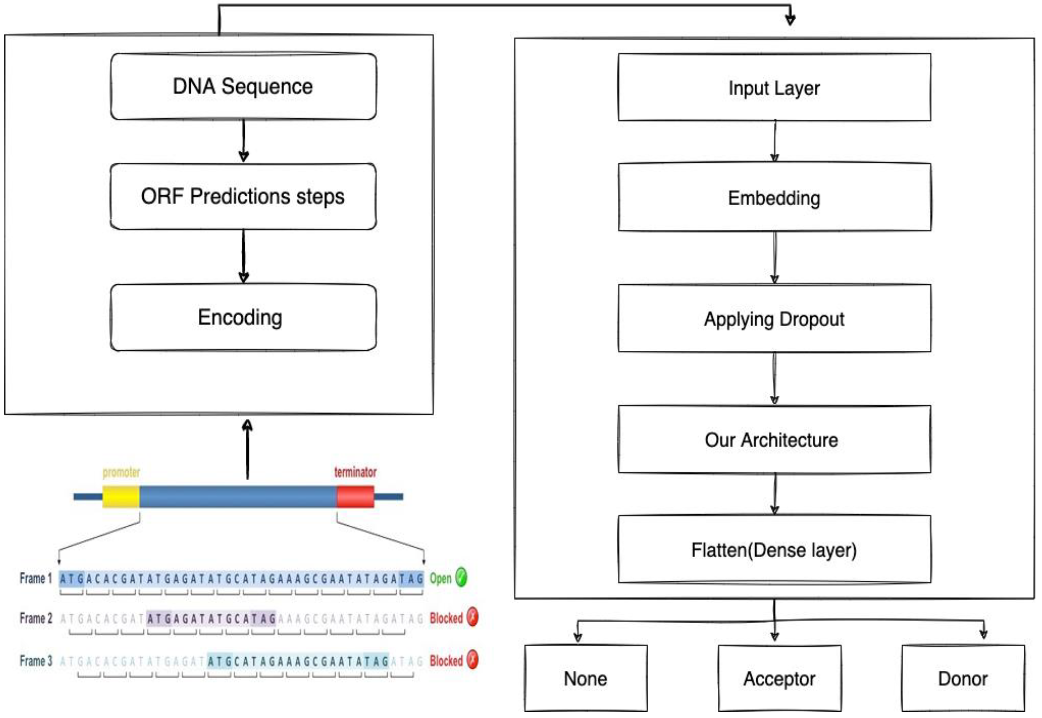
2.1.1. Identifying the Donor and Acceptor of Splice Sites

This example has previously determined the splice site donor and acceptor regions. A third zone, dubbed the Non Site Region, was included to improve the model further. The software has been created to assist in identifying the donor and acceptor. The G.T. area is the donor, whereas the A.G. region is the acceptor. Each ORF is read in as a string variable. Table 1 demonstrates that this software can locate G.T. positions beginning with G.T. and store them in an array among the other triplets in this area.

Similarly, the program hunts for the A.G. region and records its position in an array among the other A.G. region places. Each class has 37,005 sequences with a window size of 70, corresponding to the number of G.T. locations discovered. The intron begins with G.T. and finishes with A.G., implying that the total number of G.T. and A.G. positions must be equal. No-location site on the map was likewise 37,005, the average G.T. and A.G. placements. These places, however, are not real donor splice sites. All three splice site regions were created: the do-nor splice site area, the acceptor splice site region, and the no-site region. Each class has 38,021 sequences with a length of 70 nucleotides.

Thirty nucleotides were appended just before, and 40 nucleotides were inserted just after each G.T. position in the list. This results in constructing a nucleotide sequence with a window size of 70 and a G.T. region in the center. This kind of training dataset is denoted by the number 0. The area containing the Acceptor splice location.

Similarly, 40 nucleotides were inserted in the A.G. position list before and after each A.G. position. As a result, a 70-window DNA sequence with an A.G. section in the center has been constructed. One: This category of training datasets has been designated as one. When an area that is not a viable splice site is not included in an array of Non-site regions, it is referred to as a No-site region. A single file containing all of the DNA from the combined ORFs was used to create splice site classes. Each splice-DNA site’s sequence was divided into 70-word portions. Thirty nucleotides were inserted before, and thirty nucleotides were added after each location on the list of no-site sites where no-site 1 existed. Similarly, a nucleotide sequence with a window size of 70 and a no-site area in the center is constructed. This category of training datasets has been designated as number two.

Machine learning must determine how to convert all of these classes’ sequences to numbers [24]. It has been used for a long period to turn each nucleotide location in a given length of DNA into a four-dimensional binary vector, which is particularly useful for CNN [25]. Due to the study’s usage of a bidirectional LSTM-RNN and GRU. Rather than that, a categorical numeric format encoding in which A = 1, G = 2, T = 3, and C = 4 are employed for the whole DNA sequence has been used [32]. This is how it transpired: The sequences of the three preceding lists were merged, and the final list was stored to input. This is how it transpired: The lists previously mentioned were concatenated, and the resulting list was saved in output. This signifies that 80% of the total data was utilized for training and testing a model. The remaining 20% of the data was utilized to validate the model.

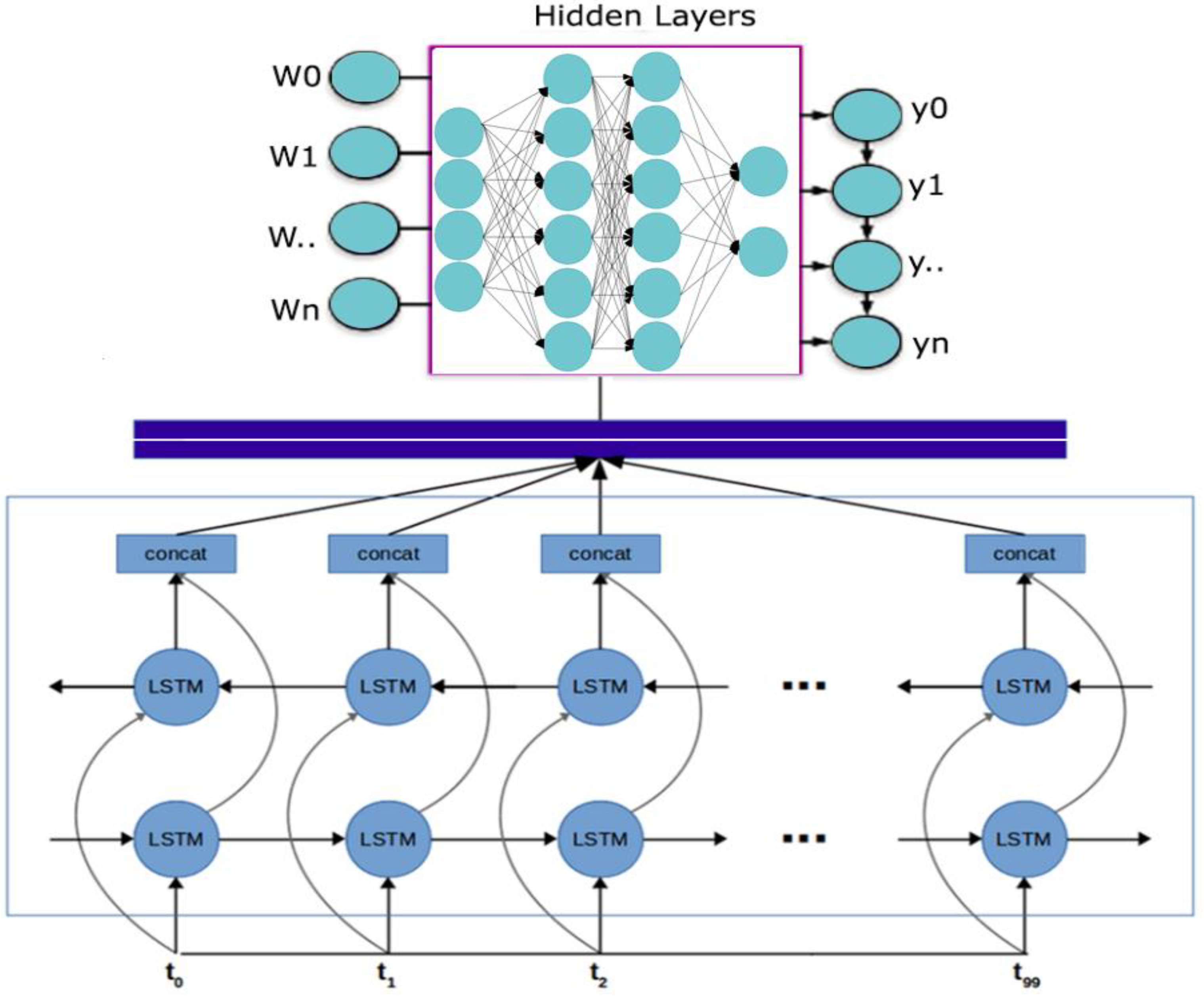
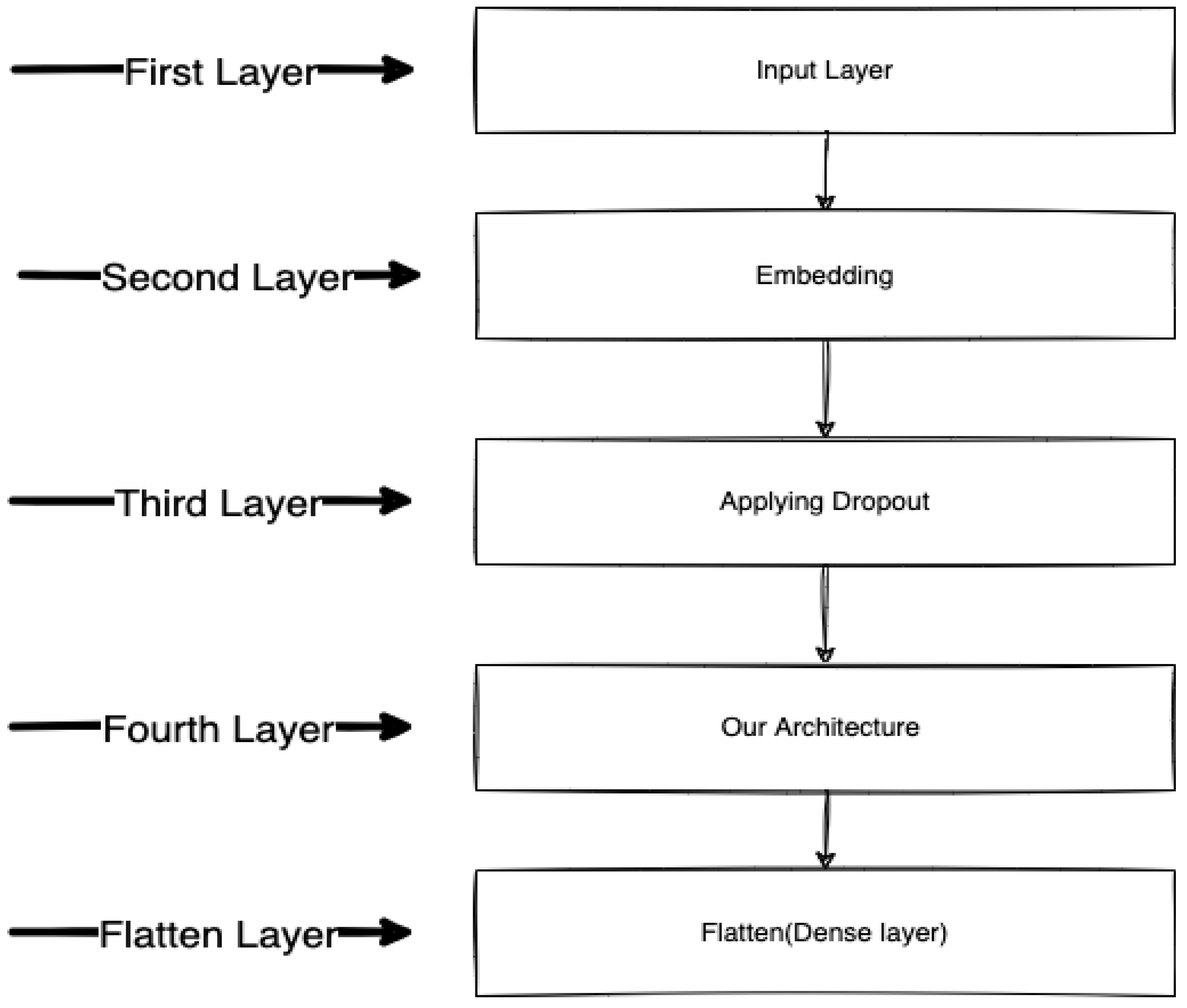
2.1.2. Bidirectional LSTM-RNN and GRU Model Preparation

A four-layer LSTM-RNN and GRU sequential model are used in this work. The first embedding layer was established with 70 and a vocabulary size of 4. It takes numeric input data. The dropout layer was implemented as the second layer, which stores only results beyond the range [33]. Then another layer is placed. It is referred to as the bidirectional LSTM layer due to its 70 inputs. The fourth layer, the dense layer, features three outputs and a softmax activation function. This layer has three outputs and a softmax activation. The softmax function, as shown, generates the probability distribution for the list classes. It is constructed using probabilistic metrics such as loss and categorical cross-entropy class, the Adam optimizer, and accuracy measures to train the model.

Table 2. Summarized bidirectional LSTM-RNN and GRU model.

Layer	Output Shapes	Parameters
Embed (input_dim)	(None, 64, 64)	400
Dropout (0.25)	(None, 64, 64)	0
Batch Normalization	(None, 128)	59,122
Flatten layer	(None, 3)	512
Total Parameters Trainable Parameters Non-Trainable Parameters	69,657
	69,647
	10

, In Keras, non-trainable parameters are the ones that are not trained using gradient descent. The trainable parameter in each layer also controls this. Trainable parameters are the number of trainable elements in the network and neurons affected by backpropagation. In comparison, non-trainable parameters are those whose value is not optimized during the training as per their gradient.

Now that all parameters except 10 are trainable, there are 10 non-trainable parameters. As layers have both trainable and non-trainable parameters, one example is the Batch Normalization layer, where the mean and standard deviation of the activations is stored for use during test time. Figure 3 displays bidirectional LSTM-RNN and GRU model represents each layer.

3. Discussion and Results

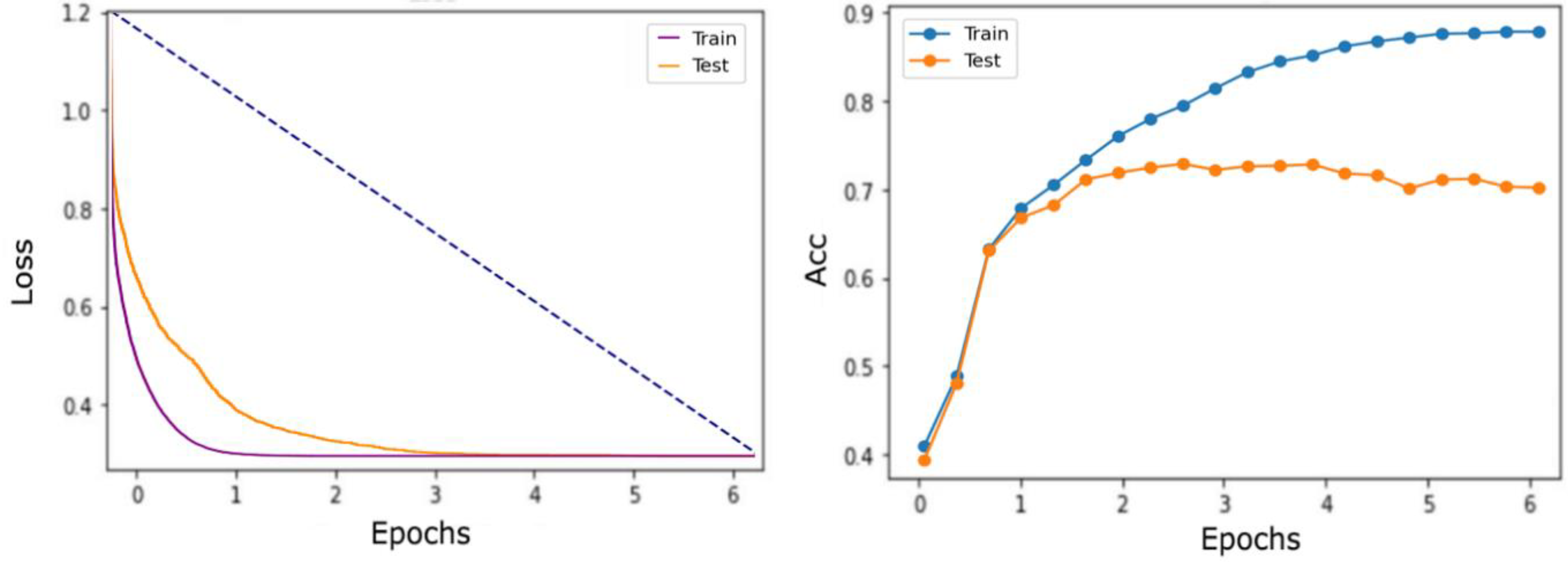
3.1. Training for Bidirectional LSTM-RNN and GRU Model

As previously stated, As previously indicated, the model was trained using around 80% of the entire dataset gathered. Train X and Train Y are the two components of the training dataset, each accounting for about 80% of the dataset. The training data for both the X and Y vectors are shown in

Table 3. Training/testing data comprised 80% and 20% of the total prepared dataset.

X/Y	Training (80%)	Testing (20%)
X_train	(88,814, 70)	(22,241, 70)
Y_train	(88,814, 3)	(22,241, 3)

. The X vector contains all nucleotide sequences with their associated window widths, whereas the Y vector has their associated labels.

The Adam optimizer in the TensorFlow library calculates the loss between true and predicted labels and accuracy measures that indicate how often predictions and labels match [34]. The model was constructed as follows: It was trained on input X, output Y, and a set of ten epochs, as well as five sets of ten epochs for each of the five times (70 epochs was the best).

Figure 4 depicts the model’s loss curves for training and test data and the accuracy curves for the training and test models. The model’s loss and accuracy improved as the number of epochs increased.

The loss curves for training and test data and the accuracy curves for training and test models are shown. As epochs rise, the model’s loss and accuracy improve.

3.2. Testing Results for the Bidirectional LSTM-RNN and GRU Model

Twenty percent of the whole dataset was used to test the model [35]. Test x and Test Y account for 20% of the dataset. Twenty percent of the testing data is used to assess the model. Table 3 contains 20% of the test data and the x and Y vectors, including all nucleotide sequences and their window size and labels. Test data is used to test the model’s ability to abstract from various sources of information. The model achieves a 96.1 percent accuracy on the test data. We tried 20:80 epochs with a cycle rate ranging from 10 to 70, and the best result was 50 cycles off 70 epochs. Before and after testing the model, a random whole genome sequence of C. parvum was used as an input sequence to predict the exons from the trained model. To improve the accuracy of intron and exon prediction, a filter based on intron length was added to the model. This increased the model’s precision.

As follows the model’s execution, it will be assigned the labels 0 and 1, and 2. This demonstrates that in a certain window of sequences, the counter indicates that 0 equals G.T., 1 equals A.G., and 2 equals no-site. This is true if a window has more than a specified number of counts for each label. It considers the intron length restriction and generates 681 introns with an average length of 89. Exons anticipated to have an average length of 1370 were predicted to have an average length of 1370. There were 4618 exons, each around 1370 words in length.

Table 4. Exons and introns are predicted by the model using genomic annotation.

	Predicted		Genome Annotation
	Exons	Introns	Exons	Introns
Number	4618	681	4231	681
Average Length	1370	89	1716	89

summarizes the suggested model’s exon and intron predictions. These predictions are compared to the annotated genome of C. parvum [36]. The length of an annotated CDS sequence for C. parvum ATCC mRNA. Due to the high gene density and small distances between genes, accurately delineating UTR boundaries using short-read sequencing data is challenging. Without assistance from the genome or reference annotation, RNA-Seq for transcriptome assembly results in a high rate of chimerism. As a result, we configured the assembly process using reference annotation and refined the parameters to decrease the amount of incorrectly fused transcripts. Due to the length limits imposed by the two fundamental splicing mechanisms, spliced exons prefer longer introns. Exons are DNA segments that contain the amino acid sequence of a gene. Most gene sequences are interrupted by one or more DNA regions termed introns in plants and animals. If an alternative exon was chosen, it was certainly included among other alternative exons discovered downstream. Thus, variants that contained one alternatively spliced exon skipped the next and then included others downstream were fairly in-frequent, accounting for 18, 14, 16, and 20% of alternatively spliced isoforms from the colon, respectively. Spliced exons are more often found in longer introns due to the length limits imposed by the two principal splicing processes for splice site pairing. Ambiguities in the gene models of all of these parasites, including transcription, start and stop sites, translation start and stop sites, and identification of introns and intron-exon borders, must be addressed.

Additionally, optimization of these genome assemblies, additional investigations to support genome annotations, and discovery and characterization of discrepancies across these genome assemblies are necessary. These genomes may help to explain variations in Cryptosporidium species traits, such as host range and pathogenicity. Our Improved Genome Annotation (IGA) revealed variations in the number of genes and intron content in C. parvum’s coding genome. The IGA identified 3865 protein-coding genes, including 74 that the OGA had overlooked [37]. Most genes lacked introns; nevertheless, whereas the OGA discovered introns in only 4.3 percent of genes, the IGA identified introns in 10.8 percent [38].

Additionally, in the revised annotation, fourteen of the OGA’s coding regions were recognized as exons belonging to nearby genes. As a result of our investigation, we found 511 extra exons and 451 additional introns previously unknown. Genes with introns typically have between two and ten exons, with an average of 2.6 exons per gene. This demonstrates that annotated C. parvum benchmark data is utilized to evaluate the model with around 96.1% accuracy.

Table 5. The suggested model’s performance was evaluated and compared to the state-of-the-art.

Model Comparison	Our Proposed Method	LSTM-RNN and GRU [30]	Bidirectional LSTM [31]	Deep Belief Networks [32]
Acc.	0.961	0.953	0.843	0.892

compares the proposed technique with the state-of-the-art, and the proposed method outperforms previous DL algorithms in predicting splice locations. Our novel bidirectional LSTM-RNN and GRU performs better than previous DL algorithms on this test. We discussed how bidirectional LSTM-RNN and GRU enable neural networks to retain forward and backward information from hidden sequences’ data states. This enables the machine to learn considerably more effectively. An RNN model is optimized for handling data presented in a sequence [28]. Only the LSTM overcomes the vanishing gradient issue and increases accuracy by increasing the number of interactions in the RNN [39].

As shown in Table 5, when we modify the condition of our computer and operate it, the network does not improve. This phenomenon is referred to as a vanishing gradient. Because the bidirectional LSTM-RNN and GRU may be employed in both directions, it was chosen for this research endeavor.

4. Conclusions

The primary goal of this work is to offer a practical approach to bidirectional LSTM-RNN and GRU for eukaryotic DNA splice site identification and estimation. Bidirectional LSTM-RNN and GRU excels in processing massive quantities of sequential data, such as the complete genome. This strategy accelerates the training of the model. The findings indicate that just 70 epochs are required to obtain a 96.1 percent accuracy level, illustrating the model’s speed. Bidirectional LSTM-RNN and GRU delivers the most accurate results. This model can predict more same exons for various eukaryotic genomes, which is an incredible accomplishment and will benefit comparative genomics research.

Some of the shortcomings in our research should be rectified. First, the LSTM-RNN and GRU is not as successful as LSTM-RNN GRU Model, and additional research is needed for non-site region, genes without the intron. Future research will explore these limitations, such as How the model deals with the longer or shorter introns and the overlapping between predicted and genome annotation results.

References

1. Kumar, A.; Chaudhry, M. Review and Analysis of Stock Market Data Prediction Using Data mining Techniques. In Proceedings of the 5th International Conference on Information Systems and Computer Networks (ISCON), Mathura, India, 22–23 October 2021; pp. 1–10. [Google Scholar]
2. Bauchet, G.J.; Bett, K.E.; Cameron, C.T.; Campbell, J.D.; Cannon, E.K.; Cannon, S.B.; Carlson, J.W.; Chan, A.; Cleary, A.; Close, T.J.; et al. The future of legume genetic data resources: Challenges, opportunities, and priorities. Legum. Sci. 2019, 1, e16. [Google Scholar] [CrossRef] [Green Version]
3. Dorrell, M.I.; Lineback, J.E. Using Shapes & Codes to Teach the Central Dogma of Molecular Biology: A Hands-On Inquiry-Based Activity. Am. Biol. Teach. 2019, 81, 202–209. [Google Scholar]
4. Smart, A. Characterizing the hnRNP Q Complex and Its Activity in Asymmetric Neural Precursor Cell Divisions during Cerebral Cortex Development. Ph.D. Thesis, University of Guelph, Guelph, ON, Canada, 2018. [Google Scholar]
5. Pudova, D.S.; Toymentseva, A.A.; Gogoleva, N.E.; Shagimardanova, E.I.; Mardanova, A.M.; Sharipova, M.R. Comparative Genome Analysis of Two Bacillus pumilus Strains Producing High Level of Extracellular Hydrolases. Genes 2022, 13, 409. [Google Scholar] [CrossRef] [PubMed]
6. Pertea, M.; Lin, X.; Salzberg, S.L. GeneSplicer: A new computational method for splice site prediction. Nucleic Acids Res. 2001, 29, 1185–1190. [Google Scholar] [CrossRef] [PubMed] [Green Version]
7. Ptok, J.; Müller, L.; Theiss, S.; Schaal, H. Context matters: Regulation of splice donor usage. Biochim. Biophys. Acta (BBA)-Gene Regul. Mech. 2019, 1862, 194391. [Google Scholar] [CrossRef] [PubMed]
8. Xing, Y.; Lee, C. Alternative splicing and RNA selection pressure—Evolutionary consequences for eukaryotic genomes. Nat. Rev. Genet. 2006, 7, 499–509. [Google Scholar] [CrossRef]
9. Roth, W.M.; Tobin, K.; Ritchie, S. Chapter 5: Learn as You Build: Integrating Science in Innovative Design. Counterpoints 2001, 177, 135–172. [Google Scholar]
10. Shoka, A.A.E.; Dessouky, M.M.; El-Sherbeny, A.S.; El-Sayed, A. Fast Seizure Detection from EEG Using Machine Learning. In Proceedings of the 7th International Japan-Africa Conference on Electronics, Communications, and Computations, (JAC-ECC), Alexandria, Egypt, 15–16 December 2019; pp. 120–123. [Google Scholar]
11. Bengio, Y.; Delalleau, O.; Roux, N. The curse of highly variable functions for local kernel machines. Adv. Neural Inf. Process. Syst. 2005, 18, 107–114. [Google Scholar]
12. Singh, N.; Katiyar, R.N.; Singh, D.B. Splice-Site Identification for Exon Prediction Using Bidirectional Lstm-Rnn Approach. Available online: https://www.ncbi.nlm.nih.gov/pmc/articles/PMC7285987/ (accessed on 21 April 2022).
13. Choi, S.; Cho, N.; Kim, K.K. Non-canonical splice junction processing increases the diversity of RBFOX2 splicing isoforms. Int. J. Biochem. Cell Biol. 2022, 144, 106172. [Google Scholar] [CrossRef]
14. Wu, Y.-C.; Feng, J.-W. Development and Application of Artificial Neural Network. Wirel. Pers. Commun. 2018, 102, 1645–1656. [Google Scholar] [CrossRef]
15. Shastri, B.J.; Tait, A.N.; de Lima, T.F.; Pernice, W.H.P.; Bhaskaran, H.; Wright, C.D.; Prucnal, P.R. Photonics for artificial intelligence and neuromorphic computing. Nat. Photon. 2021, 15, 102–114. [Google Scholar] [CrossRef]
16. Singh, N.; Nath, R.; Singh, D.B. Prediction of Eukaryotic Exons using Bidirectional LSTM-RNN based Deep Learning Model. Int. J. 2021, 9, 275–278. [Google Scholar]
17. Hapudeniya, M. Artificial Neural Networks in Bioinformatics. Sri Lanka J. Bio-Med. Inform. 2010, 1, 104. [Google Scholar] [CrossRef] [Green Version]
18. Ostmeyer, J.; Cowell, L. Machine learning on sequential data using a recurrent weighted average. Neurocomputing 2018, 331, 281–288. [Google Scholar] [CrossRef] [PubMed]
19. Baldi, P.; Brunak, S. Bioinformatics: The Machine Learning Approach. In Bioinformatics: The Machine Learning Approach; MIT Press: Cambridge, MA, USA, 2001; p. 452. [Google Scholar]
20. Kumar, J.; Goomer, R.; Singh, A.K. Long Short-Term Memory Recurrent Neural Network (LSTM-RNN) Based Workload Forecasting Model for Cloud Datacenters. Procedia Comput. Sci. 2018, 125, 676–682. [Google Scholar] [CrossRef]
21. Ramsauer, H.; Schäfl, B.; Lehner, J.; Seidl, P.; Widrich, M.; Adler, T.; Gruber, L.; Holzleitner, M.; Pavlović, M.; Sandve, G.; et al. Hopfield networks is all you need. arXiv 2020, arXiv:2008.02217. [Google Scholar]
22. Sulehria, H.K.; Zhang, Y. Hopfield Neural Networks: A Survey. In Proceedings of the 6th WSEAS International Conference on Artificial Intelligence, Knowledge Engineering and Data Bases, Corfu Island, Greece, 16–19 February 2007; Volume 6, pp. 125–130. [Google Scholar]
23. Hochreiter, S.; Schmidhuber, J. Long short-term memory. Neural Comput. 1997, 9, 1735–1780. [Google Scholar] [CrossRef]
24. El Bakrawy, L.M.; Cifci, M.A.; Kausar, S.; Hussain, S.; Islam, M.A.; Alatas, B.; Desuky, A.S. A Modified Ant Lion Optimization Method and Its Application for Instance Reduction Problem in Balanced and Imbalanced Data. Axioms 2022, 11, 95. [Google Scholar] [CrossRef]
25. Sagheer, A.; Kotb, M. Unsupervised pre-training of a deep LSTM-based stacked autoencoder for multivariate time series forecasting problems. Sci. Rep. 2019, 9, 1–16. [Google Scholar]
26. Kavitha, S.; Sanjana, N.; Yogajeeva, K.; Sathyavathi, S. Speech Emotion Recognition Using Different Activation Function. In Proceedings of the International Conference on Advancements in Electrical, Electronics, Communication, Computing and Automation (ICAECA), Kumaraguru College of Technology, Coimbatore, Tamilnadu, India, 8–9 October 2021; pp. 1–5. [Google Scholar]
27. Graves, A.; Schmidhuber, J. Framewise phoneme classification with bidirectional LSTM and other neural network architectures. Neural Netw. 2005, 18, 602–610. [Google Scholar] [CrossRef]
28. Hakkani-Tür, D.; Tür, G.; Celikyilmaz, A.; Chen, Y.N.; Gao, J.; Deng, L.; Wang, Y.Y. Multi-domain joint semantic frame parsing using bi-directional rnn-lstm. In Proceedings of the 17th Annual Meeting of the International Speech Communication Association (INTERSPEECH), San Francisco, CA, USA, 8–12 September 2016; pp. 715–719. [Google Scholar]
29. Cifci, M.A.; Aslan, Z. Deep learning algorithms for diagnosis of breast cancer with maximum likelihood estimation. In International Conference on Computational Science and Its Applications; Springer: Cham, Switzerland, 2020; pp. 486–502. [Google Scholar]
30. Lee, B.; Lee, T.; Na, B.; Yoon, S. DNA-Level Splice Junction Prediction using Deep Recurrent Neural Networks. 2015. Available online: http://arxiv.org/abs/1512.05135 (accessed on 12 February 2022).
31. Lee, T.; Yoon, S. Boosted Categorical Restricted Boltzmann Machine for Computational Prediction of Splice Junctions. 2015; pp. 2483–2492. Available online: http://proceedings.mlr.press/v37/leeb15.html (accessed on 20 March 2022).
32. Augustauskas, R.; Lipnickas, A. Pixel-level Road Pavement Defects Segmentation Based on Various Loss Functions. In Proceedings of the 11th IEEE International Conference on Intelligent Data Acquisition and Advanced Computing Systems: Technology and Applications (IDAACS), Cracow, Poland, 22–25 September 2021; Volume 1, pp. 292–300. [Google Scholar]
33. Kim, B.-H.; Pyun, J.-Y. ECG Identification for Personal Authentication Using LSTM-Based Deep Recurrent Neural Networks. Sensors 2020, 20, 3069. [Google Scholar] [CrossRef] [PubMed]
34. Nasser, M.; Salim, N.; Hamza, H.; Saeed, F.; Rabiu, I. Improved deep learning-based method for molecular similarity searching using stack of deep belief networks. Molecules 2020, 26, 128. [Google Scholar] [CrossRef] [PubMed]
35. Ning, L.; Pittman, R.; Shen, X. LCD: A Fast-Contrastive Divergence Based algorithms for Restricted Boltzmann Machine. Neural Netw. 2018, 108, 399–410. [Google Scholar] [CrossRef]
36. Cui, Z.; Ke, R.; Pu, Z.; Wang, Y. Stacked bidirectional and unidirectional LSTM recurrent neural network for forecasting network-wide traffic state with missing values. Transp. Res. Part C Emerg. Technol. 2020, 118, 102674. [Google Scholar] [CrossRef]
37. Wang, F.; Xuan, Z.; Zhen, Z.; Li, K.; Wang, T.; Shi, M. A day-ahead P.V. power forecasting method based on LSTM-RNN model and time correlation modification under partial daily pattern prediction framework. Energy Convers. Manag. 2020, 212, 112766. [Google Scholar] [CrossRef]
38. Khine, W.L.K.; Aung, N.T.T. Aspect Level Sentiment Analysis Using Bi-Directional LSTM Encoder with the Attention Mechanism. In Proceedings of the International Conference on Computational Collective Intelligence, Da Nang, Vietnam, 30 November–3 December 2020; Springer: Cham, Switzerland, 2020; pp. 279–292. [Google Scholar]
39. Jang, B.; Kim, M.; Harerimana, G.; Kang, S.U.; Kim, J.W. Bi-LSTM model to increase accuracy in text classification: Combining Word2vec CNN and attention mechanism. Appl. Sci. 2020, 10, 5841. [Google Scholar] [CrossRef]
Figure 1. The architecture of Bidirectional Long short-term memory.
Applsci 12 04390 g001
Figure 2. A bidirectional LSTM-RNN and GRU model was suggested for use in the workplan.
Applsci 12 04390 g002
Figure 3. A bidirectional LSTM-RNN and GRU model represents each layer (Abdullahi, 2022).
Applsci 12 04390 g003
Figure 4. Loss curve and accuracy with the best epoch for the training model.
Applsci 12 04390 g004