A Low-Complexity Channel Estimation Based on a Least-Squares Algorithm in OFDM Systems

Abstract

As the channel frequency responses (CFRs) at virtual pilot subcarriers are assumed to be zero, the estimated CFRs will have a leakage effect for discrete Fourier transform (DFT)-based channel estimation in OFDM systems. The CFRs at odd pilot subcarriers and even pilot subcarriers are related if the number of maximum channel delay points is smaller than or equal to half the number of pilots (including virtual pilots). According to this correlation, we propose a low-complexity least-squares (LS) method to estimate the CFRs at virtual even and odd pilot subcarriers, respectively. This will solve the problem of the leakage effect in DFT-based channel estimation. The proposed method does not need to know the statistical properties of the channel or insert extra pilots as with some estimation methods. Furthermore, although this method has less computation than the LS method, both have almost the same channel estimation efficiency in simulation. The channel estimation efficiency of our proposed method is still similar to that of the LS method, even if the number of maximum channel delay points is greater than half the number of pilots. Therefore, the proposed low-complexity method is very suitable for equalizer hardware implementation.

1. Introduction

Transmitted signals are distorted by multi-path propagation in wireless communication. Therefore, in wireless OFDM systems, equalization is popularly performed to compensate for the distorted signals. One of the most important jobs of an equalizer is CFR estimation. The communication specifications in a mobile environment are usually provided with pilots to estimate the CFR at the receiver. There are three common types of pilot signal arrangements: block arrangement, comb arrangement, and scattered arrangement [1,2,3]. In comb-type pilot arrangement, the pilot signals are uniformly distributed in the frequency domain within each OFDM symbol, while in block-type pilot arrangement, the pilot signals are assigned to all subcarriers in a particular OFDM symbol, which is sent periodically in the time domain. In scattered-type pilot arrangement, pilot signals are scattered in the time and frequency domains. The channel estimation is generally divided into two steps at the receiver. First, the CFRs at the pilot subcarriers are estimated. Second, the CFRs at the data subcarriers are estimated using the estimated CFRs at the pilot subcarriers. In the second step, the common estimation methods include 1D or 2D linear interpolation [4,5], the DFT-based channel estimation [6,7,8,9], the LS method [10,11], and the compressed sensing method [12,13,14,15,16,17]. Linear interpolation requires the least computation, while the compressed-sensing method requires the most. In recent years, machine learning has also been used for channel estimation [18,19,20,21,22]. However, these algorithms [18,19,20,21,22] are usually computationally demanding and require a large number of training samples. Refs. [23,24,25] are other related literatures we refer to.

If there is no guard band and the pilot spacing is the integer power of two for the comb-type pilot arrangement, the DFT-based channel estimation is a good estimation method. However, in the present communication specifications, there is a guard band in the spectrum to reduce the interference from neighboring bands. This leads to large errors in the estimated CFRs near the guard band based on the DFT-based channel estimation (i.e., the leakage effect [6,7,8,9]). In [6,7,8], the CFRs at the virtual pilot subcarriers were estimated with different methods. The method proposed in [6] inserts extra pilots at the specific subcarriers on both sides of the guard band. Then, the CFRs at the virtual pilot subcarriers are estimated using the inserted pilots. However, as the pilot signal arrangement used by this method is not applicable to any communication specification, it cannot be used in actual communication systems. The optimal linear estimator for leakage suppression is proposed in [7]. The method [7] must determine the statistical properties of a channel. However, in practical application, the statistical properties of a channel are unknown and unlikely to be estimated. In [8], the estimated CFRs at the two pilot subcarriers at both ends of the guard band were used to estimate CFRs at the virtual pilot subcarriers by linear interpolation. However, linear interpolation may not provide a good estimate. The three methods can estimate the overall CFR using the conventional DFT-based channel estimation after estimating the CFRs at the virtual pilot subcarriers. The two estimating channel impulse response (CIR) methods of [9,11] are very similar, and their computational complexities are the same.

The method proposed in this paper does not require any statistical properties of a channel or the insertion of extra pilots. This method is applicable to the pilot signals in a comb arrangement. When the number of maximum channel delay points is smaller than or equal to half the number of pilots (including virtual pilots), the CFRs at the virtual pilot subcarriers can be estimated. The method proposed in this paper has lower computational complexity and stored complex numbers than the LS method [11]. The channel estimation efficiency of our proposed method is still similar to that of the LS method, even if the number of maximum channel delay points is greater than half the number of pilots. Therefore, this paper performed simple system simulations in the time-varying channel to verify the channel estimation efficiency of the proposed method.

The system architecture is outlined in Section 2 and the proposed method is introduced in Section 3. The computational complexity is compared with the LS method in Section 4. Furthermore, Section 5 shows the simulation and discussion, while Section 6 shows the conclusions of this paper.

2. Pilot Arrangement and CFR Estimation at Pilot Subcarrier

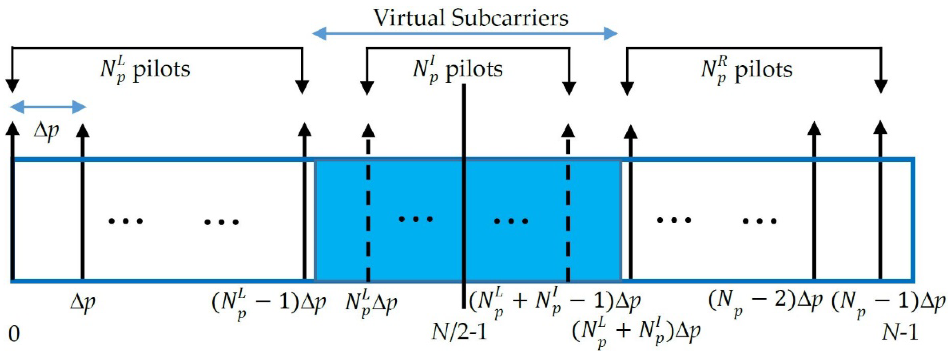
Figure 1 shows the locations of the pilot of the OFDM system with a comb-type pilot arrangement. Related parameters are described in

Table 1. Parameter definitions.

Parameter	Meaning
N	The number of FFT points.
Δp	The spacing between pilot subcarriers.
$N_P^L$	The number of pilot subcarriers on the left of the virtual subcarrier area.
$N_P^I$	The number of virtual pilot subcarriers in the virtual subcarrier area.
$N_P^R$	The number of pilot subcarriers on the right of the virtual subcarrier area.
Np	$\mathrm{The}\mathrm{total}\mathrm{number}\mathrm{of}\mathrm{pilot}\mathrm{subcarriers},\mathrm{including}\mathrm{virtual}\mathrm{pilot}\mathrm{subcarriers}(\mathrm{i}.\mathrm{e}.,N_p=N/\Delta p=N_P^L+N_P^I+N_P^R$).
$N_P^{out}$	$\mathrm{The}\mathrm{number}\mathrm{of}\mathrm{pilot}\mathrm{subcarriers}\mathrm{out}\mathrm{of}\mathrm{the}\mathrm{virtual}\mathrm{subcarrier}\mathrm{area}\mathrm{and}{N}_P^{out}=N_P^L+N_P^R$.

. When the time-varying channel is approximately invariant in an OFDM symbol, the digital CIR corresponding to some OFDM symbols will be set to h[n], where n is the index for time. If the number of maximum channel delay points is N_p/2, h[n] = 0 when n > N_p/2 − 1 or n < 0. Let the frequency domain data transferred in an OFDM symbol be X[k], where k is the index for frequency. The time-domain signal x[n] is derived from the N-points IDFT of X[k] (i.e., the content free of CP (cyclic prefix) in this OFDM symbol). Let the OFDM symbol content received by the receiver after the CP is removed be y[n]. When the CP is long enough that two adjacent OFDM symbols will not disturb each other because of the channel, y[n] can be expressed as follows:

y[n] = x[n] ⊗ h[n] + w[n],

(1)

where w[n] is white Gaussian noise and ⊗ is the circular convolution operation. The CFR H[k] of this OFDM symbol can be derived from the N-points DFT of h[n]; the mathematical expression is given as follows:

$$H[k]={\displaystyle \sum _{n=0}^{N-1}h[n]e^{-j2\pi kn/N}}={\displaystyle \sum _{n=0}^{N_p/2-1}h[n]e^{-j2\pi kn/N}},0\le k\le N-1.$$

(2)

The N-points DFTs of x[n], y[n], and w[n] are X[k], Y[k], and W[k], respectively. In addition:

$$\begin{gathered} X[k]={\displaystyle \sum _{n=0}^{N-1}x[n]e^{-j2\pi kn/N}},0\le k\le N-1, \\ Y[k]={\displaystyle \sum _{n=0}^{N-1}y[n]e^{-j2\pi kn/N}},0\le k\le N-1, \\ W[k]={\displaystyle \sum _{n=0}^{N-1}w[n]e^{-j2\pi kn/N}},0\le k\le N-1, \end{gathered}$$

where W[k] is also white Gaussian noise. The DFT of a circular convolution of two N-points sequences is the product of their respective DFTs. In an OFDM symbol, Y[k] can be expressed as follows:

Y[k] = X[k]H[k] + W[k], 0 ≤ k ≤ N − 1.

(3)

Afterward, CFRs at the pilot subcarriers are estimated by the LS method. The CFRs estimated at the pilot subcarriers can be written as follows:

$$\widehat{H}[k_p]=Y[k_p]/X[k_p]=H[k_p]+W[k_p]/X[k_p],k_p\in \mathrm{pilot}.$$

(4)

All the above variables are described in

Table 2. Variable definitions.

Variable	Meaning
h[n]	The CIR in an OFDM symbol, 0 ≤ n ≤ N − 1.
H[k]	The CFR in an OFDM symbol, 0 ≤ k ≤ N − 1.
x[n]	The time-domain data transferred in an OFDM symbol, 0 ≤ n ≤ N − 1.
X[n]	The frequency-domain data transferred in an OFDM symbol, 0 ≤ k ≤ N − 1.
y[n]	The time-domain received data in an OFDM symbol, 0 ≤ n ≤ N − 1.
Y[k]	The frequency-domain received data transferred in an OFDM symbol, 0 ≤ k ≤ N − 1.
w[n]	The time-domain noise in an OFDM symbol at receiver, 0 ≤ n ≤ N − 1.
W[k]	The frequency-domain noise in an OFDM symbol at receiver, 0 ≤ k ≤ N − 1.
$\widehat{H}[k_p]$	The estimated CFRs at pilot subcarriers, kp ∈ pilot

.

3. The Proposed Method Based on the LS Method

The number of maximum delay points of a CIR was assumed to be N_p/2. We divided the pilots into two groups according to their locations as even and odd multiples of ∆p. From (2), two groups of CFR with adjacent pilots spaced by 2∆p were first observed, i.e.,

$$H[2k\Delta p]={\displaystyle \sum _{n=0}^{N_p/2-1}h[n]e^{\frac{-j2\pi n(2k\Delta p)}{N}}},k=0,1\cdots ,N/(2\Delta p)-1,$$

(5)

$$H[\left(2k+1\right)\Delta p]={\displaystyle \sum _{n=0}^{N_p/2-1}h[n]e^{\frac{-j2\pi n\left(2k+1\right)\Delta p}{N}}},k=0,1\cdots ,N/(2\Delta p)-1.$$

(6)

The N_p/2-points of IDFTs of H[2k∆p] and H[(2k + 1)∆p] are shown as (7) and (8), respectively:

$$h[n]=\frac{2}{N_P}{\displaystyle \sum _{k=0}^{\left(N_P/2\right)-1}H[2k\Delta p]e^{\frac{j2\pi nk}{N_P/2}}},n=0,1,\dots ,N_P/2-1,$$

(7)

$$h[n]=\frac{2}{N_P}{e}^{\frac{j2\pi n}{N_P}}{\displaystyle \sum _{k=0}^{\left(N_P/2\right)-1}H[(2k+1)\Delta p]e^{\frac{j2\pi nk}{N_P/2}},}n=0,1,\dots ,N_P/2-1.$$

(8)

(7) and (8) are represented by the following matrices:

h = G_pH_p,even,

(9)

h = DG_pH_p,odd,

(10)

where

h = [h[0] h[1] … h[(N_p/2) − 1]]^T,

H_p,even = [H[0] H[2∆p] … H[(N_p − 2)∆p]]^T,

H_p,odd = [H[∆p] H[3∆p] … H[(N_p − 1)∆p]]^T,

D = diag(1,e^j2π/Np, …, e^{j2π(Np/2−1)/Np}),

G_p is the inverse Fourier transform matrix of 0.5N_p × 0.5N_p with (G_p)_i,k = 2e^{j2πik/(Np/2)}/N_p and i, k = 0, 1, 2, …, N_p/2 − 1. The CIR can be written as (9) and (10), so the two equations are equal as follows:

G_pH_p,even = DG_pH_p,odd.

(11)

The CFRs at the virtual even pilot subcarriers were selected as the target of estimation. Equation (11) was changed as follows:

H_p,odd = 0.5N_p(G_p)^HD^HG_pH_p,even = AH_p,even,

(12)

where (·)^H represents the conjugate transposed operation of a matrix; 0.5N_p${\mathbf{G}}_p^H{=\mathbf{G}}_P^{-1}$, $D^H=D^{-1}$; and A = 0.5N_p(G_p)^HD^HG_p is a 0.5N_p × 0.5N_p matrix. For convenient representation, A is expressed as follows:

$$A=\left[\begin{array}{ccc}{A}_{1(0.25N_p^{out}\times 0.25N_p^{out})}& A_{2(0.25N_p^{out}\times 0.5N_p^I)}& A_{3(0.25N_p^{out}\times 0.25N_p^{out})}\\ A_{4(0.5N_p^I\times 0.25N_p^{out})}& A_{5(0.5N_p^I\times 0.5N_p^I)}& A_{6(0.5N_p^I\times 0.25N_p^{out})}\\ A_{7(0.25N_p^{out}\times 0.25N_p^{out})}& A_{8(0.25N_p^{out}\times 0.5N_p^I)}& A_{9(0.25N_p^{out}\times 0.25N_p^{out})}\end{array}\right]$$

(13)

In this case, we assume that $N_P^L$ and $N_P^R$ are both even and equal and $N_P^{out}$ is a multiple of 4. So $N_P^I$ is also even. Otherwise, the matrix dimensions of A₁ to A₉ will vary according to different conditions. As the target of estimation is the CFRs at the virtual even pilot subcarriers, the unknown CFRs at the virtual subcarriers part in the left term H_p,odd of (12) were removed, and the equation at the righthand side of (12) was divided into two parts: CFRs at virtual and non-virtual pilot subcarriers. Equation (12) can be changed to the following:

$$H_{p,odd}^{out}-A_{C,R}^{out,out}{H}_{p,even}^{out}=A_{C,R}^{out,in}{H}_{p,even}^{in}$$

(14)

where

$$\begin{gathered} {\mathbf{H}}_{p,odd}^{out}={\left[\begin{array}{cccccccc}H[\Delta p]& H[3\Delta p]& \cdots & H[(N_P^L-1)\Delta p]& H[(N_P^L+N_P^I+1)\Delta p]& H[(N_P^L+N_P^I+3)\Delta p]& \cdots & H[(N_P-1)\Delta p]\end{array}\right]}^T, \\ {\mathbf{H}}_{p,even}^{out}={\left[\begin{array}{cccccccc}H[0]& H[2\Delta p]& \cdots & H[(N_P^L-2)\Delta p]& H[(N_P^L+N_P^I)\Delta p]& H[(N_P^L+N_P^I+2)\Delta p]& \cdots & H[(N_P-2)\Delta p]\end{array}\right]}^T, \\ {\mathbf{H}}_{p,even}^{in}={\left[\begin{array}{cccc}H[N_P^L\Delta p]& H[(N_P^L+2)\Delta p]& \cdots & H[(N_P^L+N_P^I-2)\Delta p]\end{array}\right]}^T. \end{gathered}$$

$H_{p,even}^{in}$ is the CFR vector at the virtual even pilot subcarriers that we aimed to estimate. $A_{C,R}^{out,out}$ is a 0.5$N_P^{out}$ × 0.5$N_P^{out}$ matrix and

$$A_{C,R}^{out,out}=\left[\begin{array}{cc}{A}_1& A_3\\ A_7& A_9\end{array}\right].$$

$A_{C,R}^{out,in}$ is a 0.5$N_P^{out}$ × 0.5$N_P^I$ matrix and

$$A_{C,R}^{out,in}=\left[\begin{array}{c}{A}_2\\ A_8\end{array}\right].$$

$H_{p,odd}^{out}$ and $H_{p,even}^{out}$ in Equation (14) can be estimated using pilot signals. $A_{C,R}^{out,out}$ and $A_{C,R}^{out,in}$ are two known matrices. Afterward, the LS method was used to estimate the CFRs at the virtual even pilot subcarriers, expressed as follows:

$${\widehat{H}}_{p,even}^{in}={[{(A_{C,R}^{out,in})}^H{A}_{C,R}^{out,in}]}^{-1}{(A_{C,R}^{out,in})}^H({\widehat{H}}_{p,odd}^{out}-A_{C,R}^{out,out}{\widehat{H}}_{p,even}^{out})$$

(15)

where ${\widehat{H}}_{p,even}^{out}$ and ${\widehat{H}}_{p,odd}^{out}$ are the CFRs estimated by (4).

There is a problem in (15), where ${(A_{C,R}^{out,in})}^H{A}_{C,R}^{out,in}$ approaches a singular matrix, so that the operation content value of the inverse matrix is abnormally large. The estimation error induced by noise will be amplified severely [11], influencing the effectiveness of this method. The corresponding improvement method has been proposed in [11], that is, to add the regularization parameter before the calculation of the inverse matrix. Thus, Equation (15) was changed to:

$${\tilde{H}}_{p,even}^{in}={[{(A_{C,R}^{out,in})}^H{A}_{C,R}^{out,in}+{\alpha }_{e}I]}^{-1}{(A_{C,R}^{out,in})}^H({\widehat{H}}_{p,odd}^{out}-A_{C,R}^{out,out}{\widehat{H}}_{p,even}^{out})$$

(16)

where α_e is the regularization parameter, which is a constant; I is a $0.5N_P^I\times 0.5N_P^I$ identity matrix; and ${\tilde{H}}_{p,even}^{in}$ is the final result estimated with the regularization parameter. However, (16) is not directly used for operation in actual hardware realization. The right side of Equation (16) was expanded as follows:

$${\tilde{H}}_{p,even}^{in}={[{({\mathbf{A}}_{C,R}^{out,in})}^H{\mathbf{A}}_{C,R}^{out,in}+{\alpha }_e\mathbf{I}]}^{-1}{({\mathbf{A}}_{C,R}^{out,in})}^H{\widehat{H}}_{p,odd}^{out}-{[{({\mathbf{A}}_{C,R}^{out,in})}^H{\mathbf{A}}_{C,R}^{out,in}+{\alpha }_e\mathbf{I}]}^{-1}{({\mathbf{A}}_{C,R}^{out,in})}^H{\mathbf{A}}_{C,R}^{out,out}{\widehat{H}}_{p,even}^{out}$$

(17)

${[{(A_{C,R}^{out,in})}^H{A}_{C,R}^{out,in}+{\alpha }_{e}I]}^{-1}{(A_{C,R}^{out,in})}^H$ and ${[{(A_{C,R}^{out,in})}^H{A}_{C,R}^{out,in}+{\alpha }_{e}I]}^{-1}{(A_{C,R}^{out,in})}^H{A}_{C,R}^{out,out}$ can be worked out in advance and stored in the memory. Both of them are $0.5N_p^I\times 0.5N_p^{out}$ matrices, and each has $0.25N_p^I{N}_p^{out}$ complex numbers to be stored in the memory. The number of multiplication operations required by (17) is much smaller than that required by (16).

Afterward, the CFRs at the virtual odd pilot subcarriers were estimated. Equation (11) was changed as in Equation (12) to obtain the following equation:

H_p,even = 0.5N_p(G_p)^HDG_pH_p,odd = BH_p,odd,

(18)

where B is a 0.5N_p × 0.5N_p matrix and B = 0.5N_p(G_p)^HDG_p. For convenient representation, B is expressed as follows:

$$B=\left[\begin{array}{ccc}{B}_{1(0.25N_p^{out}\times 0.25N_p^{out})}& B_{2(0.25N_p^{out}\times 0.5N_p^I)}& B_{3(0.25N_p^{out}\times 0.25N_p^{out})}\\ B_{4(0.5N_p^I\times 0.25N_p^{out})}& B_{5(0.5N_p^I\times 0.5N_p^I)}& B_{6(0.5N_p^I\times 0.25N_p^{out})}\\ B_{7(0.25N_p^{out}\times 0.25N_p^{out})}& B_{8(0.25N_p^{out}\times 0.5N_p^I)}& B_{9(0.25N_p^{out}\times 0.25N_p^{out})}\end{array}\right]$$

(19)

As the target of estimation is the CFRs at the virtual odd pilot subcarriers, the unknown CFRs at the virtual subcarriers part in the left term H_p,even of (18) were removed, and the equation at the right-hand side of (18) was divided into two parts: CFRs at virtual and non-virtual pilot subcarriers. Equation (18) can be changed to the following:

$$H_{p,even}^{out}-B_{C,R}^{out,out}{H}_{p,odd}^{out}=B_{C,R}^{out,in}{H}_{p,odd}^{in}$$

where

$${\mathrm{H}}_{p,odd}^{in}={\left[\begin{array}{cccc}H[(N_P^L+1)\Delta p]& H[(N_P^L+3)\Delta p]& \cdots & H[(N_P^L+N_P^I-1)\Delta p]\end{array}\right]}^T$$

$H_{p,odd}^{in}$ is the CFR vector at the virtual odd pilot subcarriers that we aimed to estimate. $B_{C,R}^{out,out}$ is a 0.5$N_P^{out}$ × 0.5$N_P^{out}$ matrix and

$$B_{C,R}^{out,out}=\left[\begin{array}{cc}{B}_1& B_3\\ B_7& B_9\end{array}\right].$$

$B_{C,R}^{out,in}$ is a 0.5$N_P^{out}$ × 0.5$N_P^I$ matrix and

$$B_{C,R}^{out,in}=\left[\begin{array}{c}{B}_2\\ B_8\end{array}\right].$$

$B_{C,R}^{out,out}$ and $B_{C,R}^{out,in}$ are two known matrices. Afterward, the LS method was used to estimate the CFRs at virtual odd pilot subcarriers, expressed as follows:

$${\tilde{H}}_{p,odd}^{in}={[{(B_{C,R}^{out,in})}^H{B}_{C,R}^{out,in}+{\alpha }_{o}I]}^{-1}{(B_{C,R}^{out,in})}^H({\widehat{H}}_{p,even}^{out}-B_{C,R}^{out,out}{\widehat{H}}_{p,odd}^{out})$$

(20)

where ${\widehat{H}}_{p,even}^{out}$ and ${\widehat{H}}_{p,odd}^{out}$ are the CFRs estimated by (4). The regularization parameter α_o is used to overcome the problem that ${(B_{C,R}^{out,in})}^H{B}_{C,R}^{out,in}$ approaches a singular matrix. Equation (20) was not directly used in actual hardware implementation. The right side of Equation (20) was expanded as follows:

$${\tilde{H}}_{p,odd}^{in}={[{(B_{C,R}^{out,in})}^H{B}_{C,R}^{out,in}+{\alpha }_{o}I]}^{-1}{(B_{C,R}^{out,in})}^H{\widehat{H}}_{p,even}^{out}-{[{(B_{C,R}^{out,in})}^H{B}_{C,R}^{out,in}+{\alpha }_{o}I]}^{-1}{(B_{C,R}^{out,in})}^H{B}_{C,R}^{out,out}{\widehat{H}}_{p,odd}^{out}$$

(21)

${[{(B_{C,R}^{out,in})}^H{B}_{C,R}^{out,in}+{\alpha }_{o}I]}^{-1}{(B_{C,R}^{out,in})}^H$ and ${[{(B_{C,R}^{out,in})}^H{B}_{C,R}^{out,in}+{\alpha }_{o}I]}^{-1}{(B_{C,R}^{out,in})}^H{B}_{C,R}^{out,out}$ can be calculated in advance and stored in the memory. Both of them are $0.5N_p^I\times 0.5N_p^{out}$ matrices, and each has $0.25N_p^I{N}_p^{out}$ complex numbers to be stored in the memory. The number of multiplication operations required by (21) is much smaller than that required by (20).

According to the results of (4), (17), and (21), the CFRs vector ${\widehat{H}}_{p,PLS}$ at the pilot and virtual pilot subcarriers can be obtained. The CIR ${\widehat{h}}_{PLS}$ of the N_p points can be calculated by the N_p-points IFFT of ${\widehat{H}}_{p,PLS}$. According to the assumptions of this paper, the number of maximum delay points of a CIR is smaller than or equal to half the number of pilots (including virtual pilot) (i.e., 0.5N_p points). Therefore, the values of 0.5N_p points of the second half of ${\widehat{h}}_{PLS}$ can be regarded as the estimation error and discarded; that is, let the values of 0.5N_p points of the second half of ${\widehat{h}}_{PLS}$ be zero to obtain ${\tilde{h}}_{PLS}$. The complete CFR ${\widehat{H}}_{PLS}$ can be obtained by N-points DFT of ${\tilde{h}}_{PLS}$.

The whole procedure of the proposed method in every OFDM symbol is organized as follows:

Step 1.

The CFRs at pilot subcarriers are estimated by (4).

Step 2.

The CFRs at virtual even and odd pilot subcarriers are estimated by (17) and (21) respectively.

Step 3.

According to step 1 and step 2, the CFRs vector ${\widehat{H}}_{p,PLS}$ at pilot and virtual pilot subcarriers can be obtained.

Step 4.

The CIR ${\widehat{h}}_{PLS}$ of the N_p points can be calculated by the N_p-points IFFT of ${\widehat{H}}_{p,PLS}$.

Step 5.

Set the values of 0.5N_p points of the second half of ${\widehat{h}}_{PLS}$ be zero to obtain ${\tilde{h}}_{PLS}$.

Step 6.

The complete CFR ${\widehat{H}}_{PLS}$ can be obtained by N-points DFT of ${\tilde{h}}_{PLS}$.

4. Comparison of Computational Complexity with the LS Method

The equation for the estimation of a CIR by the LS method in [11] is shown as follows:

$${\widehat{h}}_{LS}={({(F_P^{out})}^H{F}_P^{out}+\alpha I)}^{-1}{(F_P^{out})}^H{\widehat{H}}_P^{out}$$

(22)

where $F_P^{out}$ is an $N_P^{out}\times N_P^{out}$ partial Fourier transform matrix with ${(f_P^{out})}_{k,n}=e^{-j2\pi nk/N}$, k ∈ pilot, n = 0, 1, …, $N_P^{out}$ − 1. Additionally, I is an $N_P^{out}\times N_P^{out}$ identity matrix. When the relevant parameters are determined, ${({(F_P^{out})}^H{F}_P^{out}+\alpha I)}^{-1}{(F_P^{out})}^H$ of (22) can be calculated in advance and stored in the memory. The acceptable channel maximum delay of the LS method is $N_P^{out}$. The channel maximum delay of our method is less than or equal to N_p/2. For a fair comparison of our method with the LS method [11], let the channel maximum delay be equal to N_p/2. Therefore, the content of ${({(F_P^{out})}^H{F}_P^{out}+\alpha I)}^{-1}{(F_P^{out})}^H$ in (22) will change, and the matrix dimension changes to 0.5$N_p\times N_P^{out}$ and has 0.5$N_p{N}_p^{out}$ complex numbers to be stored in the memory. The computational complexity of Equation (22) is $0.5N_p{N}_p^{out}$ complex multiplications.

Consider the number of multiplications after CFRs estimation at the pilot subcarriers until the CIR estimation. The computation of our method was divided into two parts. Part 1 uses (17) and (21) to estimate the CFRs at the virtual pilot subcarriers. The number of multiplications of this part is $N_P^{out}{N}_P^I$. Part 2 performs the N_p-points IFFT to obtain the CIR. The number of multiplications of this part is (N_p/2)log₂(N_p) [26]. Therefore, the computation of the proposed method requires $N_P^{out}{N}_P^I$ + (N_p/2)log₂(N_p) complex multiplications, which is much fewer than $0.5N_p{N}_p^{out}$ in general cases. Comparisons with relevant parameters are described in subsequent simulations.

5. Simulation and Discussion

First, the simulation parameters were set up in

Table 3. Simulation parameters.

Parameter	Specification
N	2048 points
CP length	128 points
Δp	16 subcarriers
Np	128 subcarriers
$N_P^{out}$	108 subcarriers
$N_P^L$	54 subcarriers
$N_P^R$	54 subcarriers
$N_P^I$	20 subcarriers
Sampling frequency fs	10 MHz
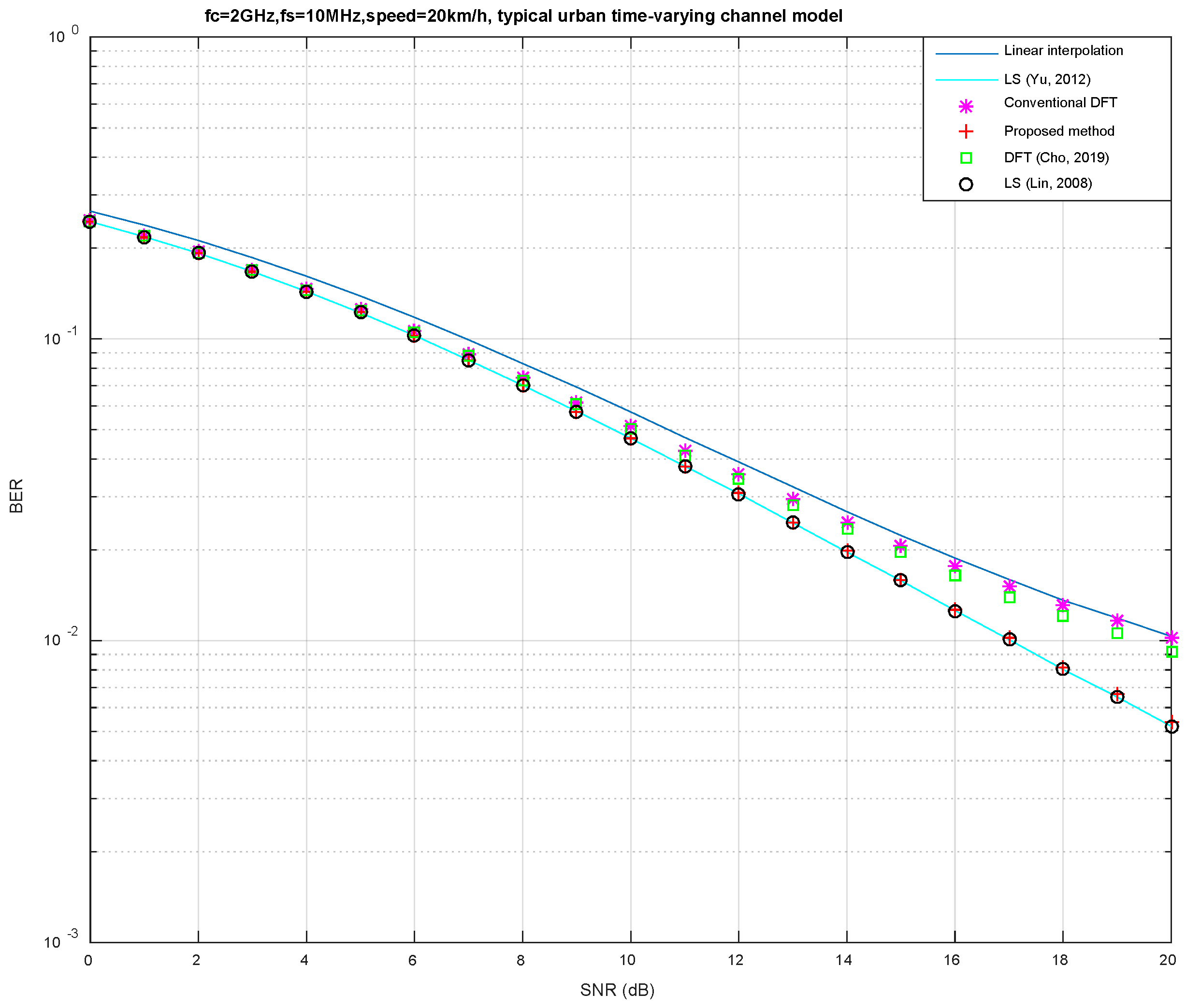
Carrier frequency fc	2 GHz

. The signal was QPSK modulation and the speed was 20 km/h.

Table 4. The typical urban time-varying channel model.

Path No. (l)	Propagation Delay	Path Power	Path Power (dB)	PSD
0	0.0 μs	0.5	−3	Jakes
1	0.2 μs	1	0	Jakes
2	0.5 μs	0.63	−2	Jakes
3	1.6 μs	0.25	−6	Gauss I
4	2.3 μs	0.16	−8	Gauss II
5	5.0 μs	0.1	−10	Gauss II

shows the typical urban time-varying channel model [27]. The three power spectral density function models were Jakes, Gauss I, and Gauss II (see COST 207 specification [27]). Forty channels were generated randomly with the channel model for simulation with different SNRs. Fifty OFDM symbols were transferred in one simulation. In terms of regularization parameters, the LS method [11] selects 0.01, while the method proposed in this paper selects α_e = α_o = 0.02. The dimension of the estimated CIR for the LS method [10] is also set to N_p/2. The problem of the matrix approaching singularity also exists in [10], so we use a regularization parameter that is set to 0.00001 to avoid this issue. The regularization parameter selection process refers to [28]. To ensure a fair comparison of the conventional DFT-based channel estimation with other methods, we only use first 0.5N_p points of the CIR estimated by conventional DFT-based channel estimation. All simulations were performed using MATLAB software.

Figure 2 is the simulated diagram of SNR to the bit error rate (BER). It is observed that the curves of the LS methods [10,11] and the method proposed in this paper are completely overlapped under the appropriate regularization parameter, meaning the BERs are very close. The BER curves of conventional DFT-based channel estimation and [8] are very close. This shows that the leakage effect was not improved by the method proposed in [8]. The conventional DFT-based channel estimation and [8] have lower computational complexity than the proposed method in this paper. However, the BER simulation showed that the proposed method has better effectiveness than the conventional DFT-based channel estimation and [8]. At low SNR, the effect of noise is higher than the leakage for the conventional DFT-based channel estimation. Therefore, the three curves of the conventional DFT, LS, and proposed methods are very close at low SNR. At high SNR, the effect of leakage is higher than the noise for the conventional DFT-based channel estimation. Therefore, the BER curve of the conventional DFT-based method is worse than the BER curves of the LS methods and the proposed method at high SNR. Linear interpolation has the lowest computational complexity but the worst BER curve.

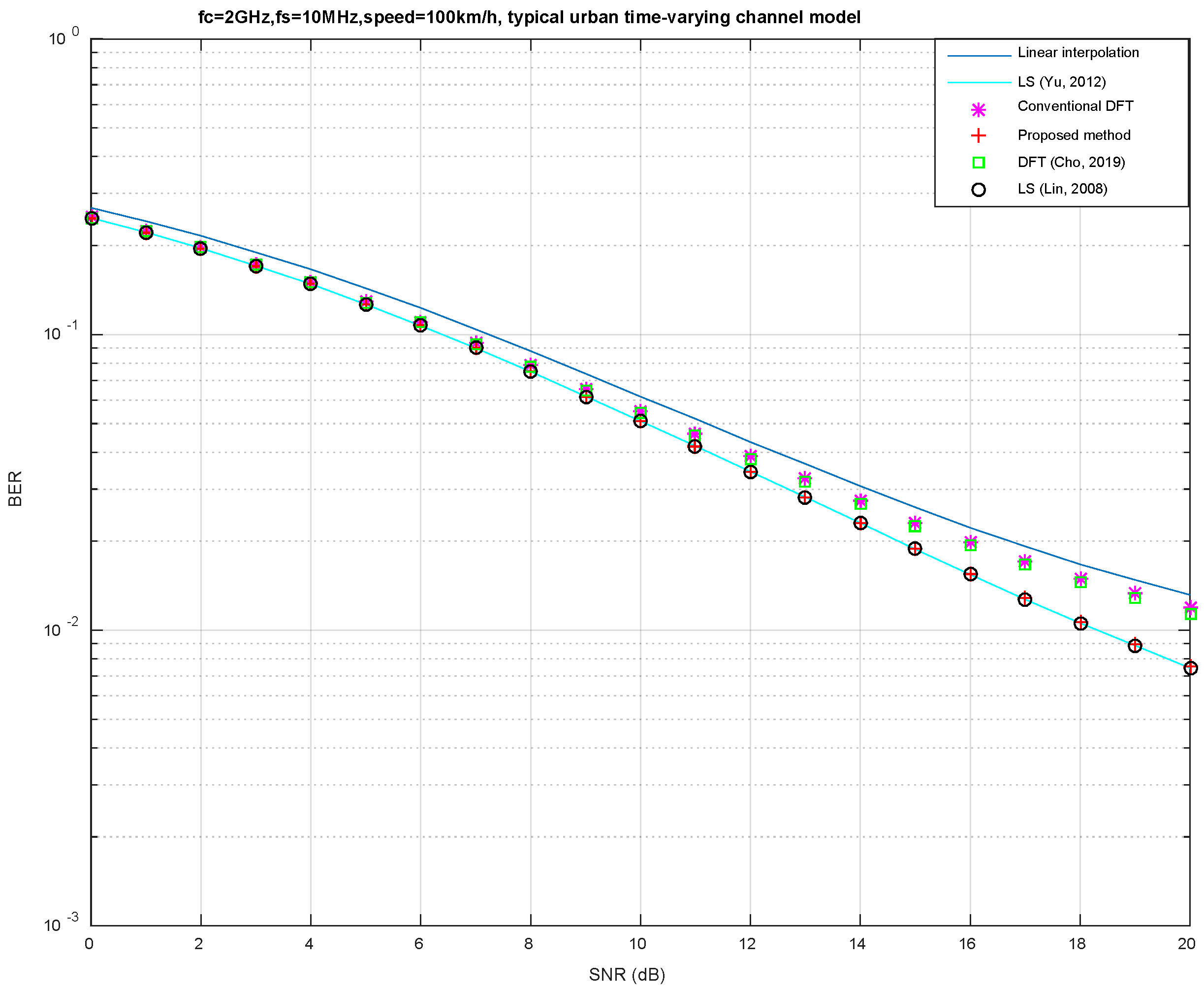
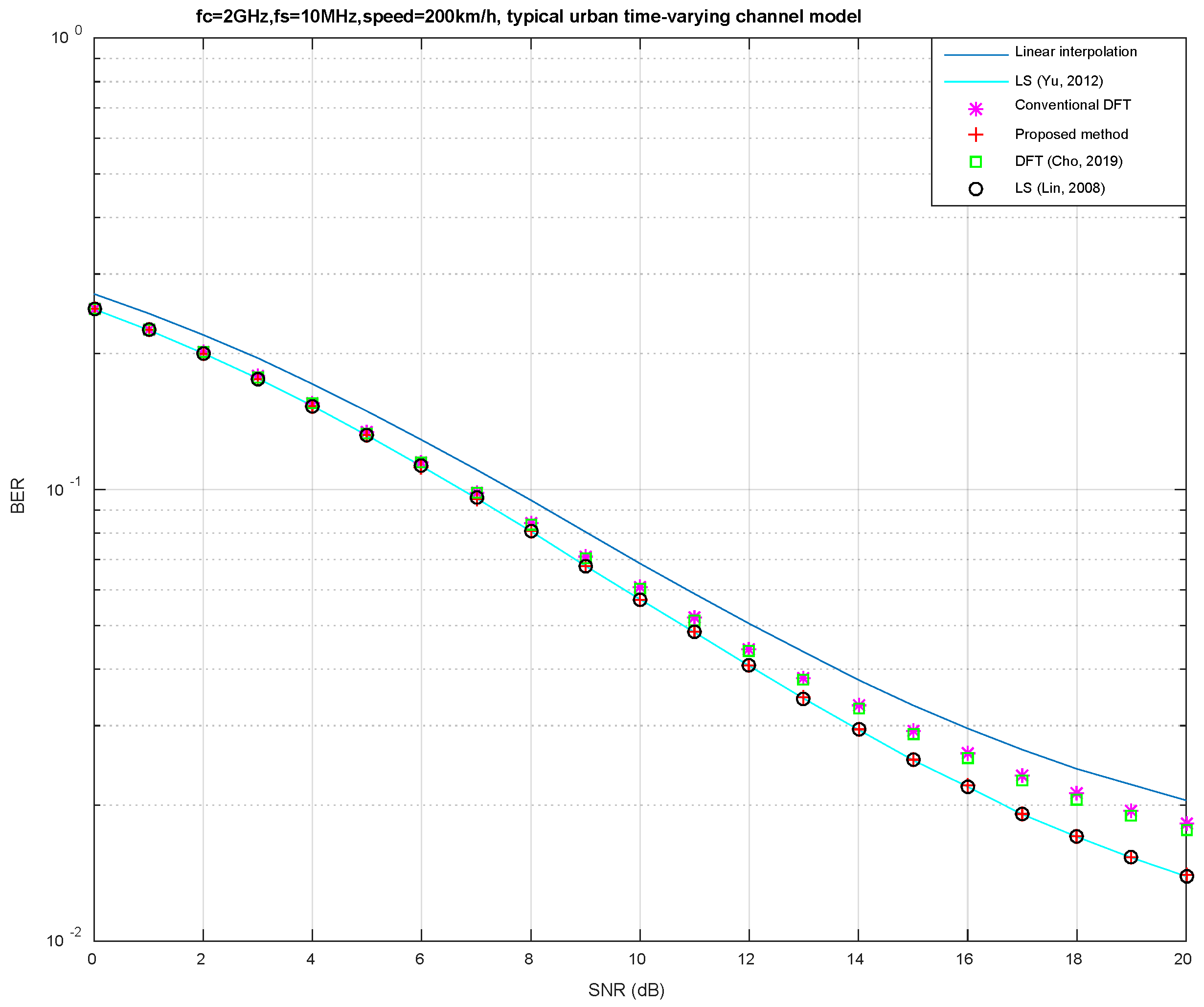
Figure 3 and Figure 4 show the simulation results with speeds equal to 100 km/h and 200 km/h, respectively. At low SNR, the six curves did not change from Figure 2, Figure 3 and Figure 4 as the effect of noise was higher than speed. At high SNR, the six curves from Figure 2, Figure 3 and Figure 4 all deteriorated with increasing speed as the effect of speed was higher than noise. Since the channel changes were extraordinarily slow, it can be assumed that the channel is approximately invariant within an OFDM symbol when speed is very low. The channel was no longer approximately invariant within an OFDM symbol when the speed is very high. Therefore, the simulation results at high speed are worse than the simulation results at low speed when SNR is high. The BER curves of the LS methods [10,11] and the method proposed in this paper are still overlapped in Figure 3 and Figure 4.

Consider the number of multiplications after CFRs at pilot subcarriers estimation until the CIR estimation. The number of complex multiplications of the LS method [11] is $0.5N_p{N}_p^{out}$. There are 6848 complex multiplications after the relevant parameters are substituted in. Meanwhile, the number of complex multiplications of the method proposed in this paper is $N_P^{out}{N}_p^I$ + (N_p/2)log₂(N_p). There are 2695 complex multiplications after the relevant parameters are substituted in. Both the LS method [11] and the proposed method have some complex numbers that need to be stored in the memory. The numbers of complex numbers that need to be stored in the memory are $0.5N_p{N}_p^{out}$ and $N_p^{out}{N}_p^I$, respectively. In this example, $0.5N_p{N}_p^{out}$ = 6848 and $N_p^{out}{N}_p^I$ = 2247.

Table 5. Comparisons of different methods on computational complexity and memory resource usage.

Method	Complex Multiplication		Stored Complex Number
	Number	Example	Number	Example
Our method	$N_P^{out}{N}_P^I$ + (Np/2)log2(Np)	2695	$N_P^{out}{N}_P^I$	2247
[9,11]	$0.5N_p{N}_p^{out}$	6848	$0.5N_p{N}_p^{out}$	6848

shows the comparisons of different methods on computational complexity and memory resource usage.

It is obvious that the method proposed in this paper has lower computational complexity and stored complex numbers than the LS method [9,11], while both have the same BER from simulations. Therefore, the method proposed in this paper is better than the LS method [9,11].

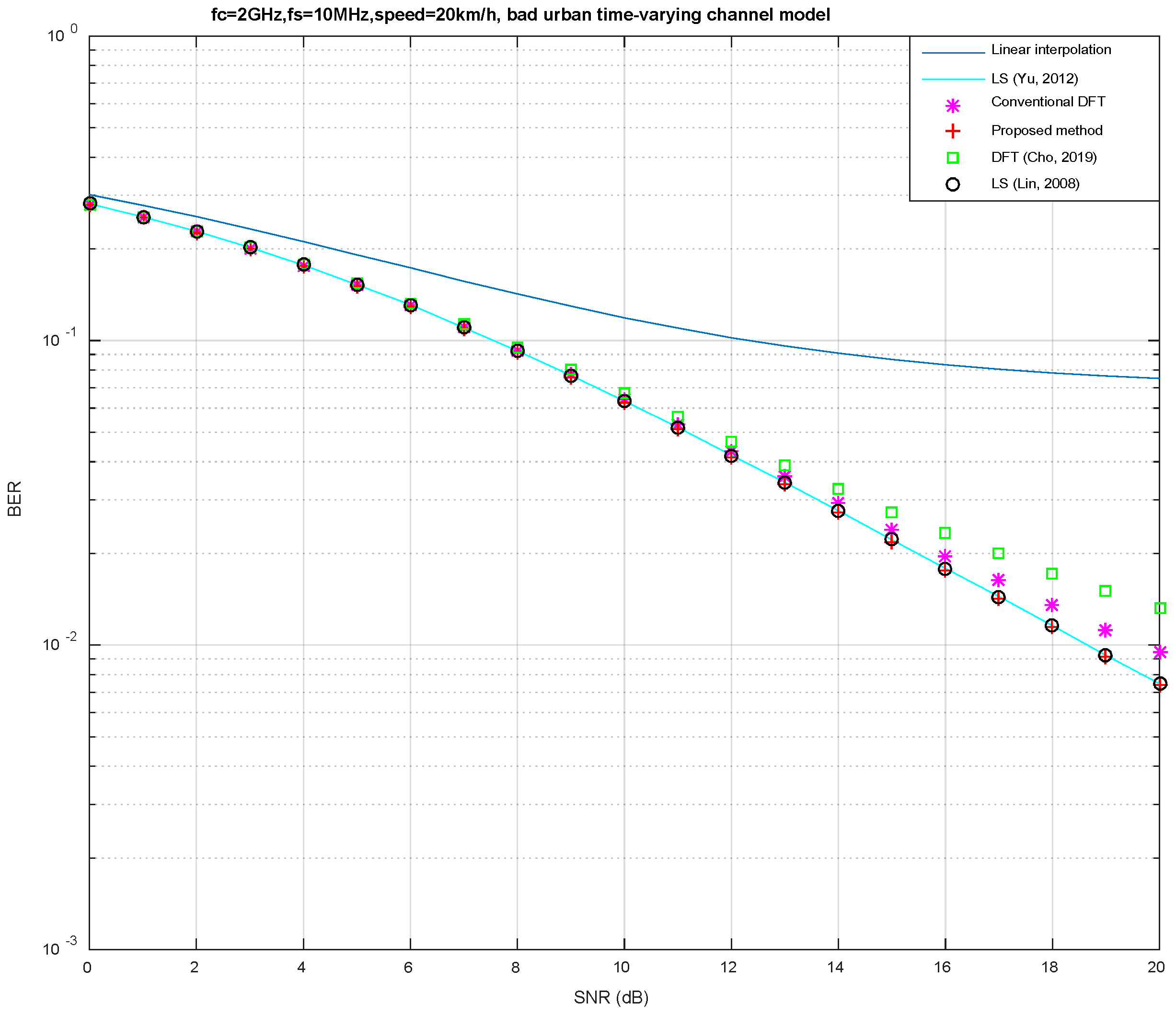
Let us consider a bad urban time-varying channel model [27] as shown in

Table 6. The bad urban time-varying channel model.

Path No. (l)	Propagation Delay	Path Power	Path Power (dB)	PSD
0	0.0 μs	0.17	−7.7	Jakes
1	0.1 μs	0.46	−3.4	Jakes
2	0.3 μs	0.74	−1.3	Jakes
3	0.7 μs	1	0	Gauss I
4	1.6 μs	0.59	−2.3	Gauss I
5	2.2 μs	0.28	−5.6	Gauss II
6	3.1 μs	0.18	−7.4	Gauss II
7	5.0 μs	0.72	−1.4	Gauss II
8	6.0 μs	0.69	−1.6	Gauss II
9	7.2 μs	0.21	−6.7	Gauss II
10	8.1 μs	0.1	−9.8	Gauss II
11	10.0 μs	0.03	−15.1	Gauss II

. The number of maximum channel delay points is equal to 100 and greater than N_p/2. Therefore, the dimension of the estimated CIR for both LS methods [10,11] is set to the maximum value of the dimension, which is $N_P^{out}$. But in this case, the matrices in both LS methods [10,11] are getting closer and closer to singular. The regularization parameters of [10,11] are set to 0.00005 and 0.05, respectively. For fair comparison, the proposed method, the DFT method, and [8] also take the first $N_P^{out}$ points of the estimated channel impulse response as the final estimated channel impulse response. Figure 5 shows the simulation results with speed equal to 20 km/h. The six curves in Figure 5 are all becoming worse than those in Figure 2. The numbers of maximum channel delay points in bad and typical urban channel models are 100 and 50, respectively. The larger the maximum channel delay, the worse the channel estimation efficiency of linear interpolation will be. Therefore, the linear interpolation curve in Figure 5 is obviously much worse than that in Figure 2. Since the matrices are getting closer and closer to singular in the two LS methods, although the regularization parameter is used, it still makes the two LS curves in Figure 5 worse than those in Figure 2. The estimated CFRs at the virtual pilot subcarriers with our proposed method will be inaccurate when the number of maximum channel delay points is larger than N_p/2. Therefore, the curve of our proposed method in Figure 5 becomes worse than that in Figure 2. However, the curves of the two LS methods and our proposed method still overlap in Figure 5. This shows the channel estimation efficiency of our proposed method is still similar to those of the LS methods [10,11], even if the number of maximum channel delay points is greater than N_p/2.

6. Conclusions

The CFRs at the odd pilot subcarriers and even pilot subcarriers are related if the number of maximum channel delay points is smaller than or equal to half the number of pilots (including virtual pilots). According to this correlation, we propose a low-complexity LS method to estimate the CFRs at the virtual even and odd pilot subcarriers, respectively. The adverse effect of unknown CFRs at the virtual pilot subcarriers for the conventional DFT-based channel estimation can be solved to enhance the channel estimation effectiveness of DFT-based channel estimation. While the channel estimation effectiveness of the proposed method is very similar to those of the LS methods [10,11], it is noteworthy that the former’s computational complexity is much lower than that of the LS method [11]. The proposed method does not need to know the statistical properties of the channel or insert extra pilots, as with some estimation methods. The channel estimation efficiency of our proposed method is still similar to those of the LS methods [10,11], even if the number of maximum channel delay points is greater than half the number of pilots. Therefore, the low-complexity method proposed in this paper is very suitable for equalizer hardware implementation.

Our proposed method has its drawbacks. It can only be applied to the comb-type pilot arrangement and the pilot spacing is the integer power of two. The two LS methods [10,11] are applicable in both comb-type and scattered-type pilot arrangements, and pilot spacing does not need to be the integer power of two.

References

1. Hsieh, M.-H.; Wei, C.-H. Channel Estimation for OFDM Systems Based on Comb-Type Pilot Arrangement in Frequency Selective Fading Channels. IEEE Trans. Consum. Electron. 1998, 44, 217–225. [Google Scholar] [CrossRef] [Green Version]
2. Coleri, S.; Ergen, M.; Puri, A.; Bahai, A. Channel Estimation Techniques Based on Pilot Arrangement in OFDM Systems. IEEE Trans. Broadcast. 2002, 48, 223–229. [Google Scholar] [CrossRef] [Green Version]
3. Choi, J.-W.; Lee, Y.-H. Optimum Pilot Pattern for Channel Estimation in OFDM Systems. IEEE Trans. Wirel. Commun. 2005, 5, 2083–2088. [Google Scholar] [CrossRef]
4. Dong, X.; Lu, W.-S.; Anthony, C.K. Linear Interpolation in Pilot Symbol Assisted Channel Estimation for OFDM. IEEE Trans. Wirel. Commun. 2007, 6, 1910–1920. [Google Scholar] [CrossRef] [Green Version]
5. Said, F.; Aghvami, H. Linear two dimensional pilot assisted channel estimation for OFDM systems. In Proceedings of the Sixth IEE Conference on Telecommunications, Edinburgh, UK, 29 March–1 April 1998; pp. 32–36. [Google Scholar]
6. Kwak, K.; Lee, S.; Kim, J.; Hong, D. A New DFT-Based Channel Estimation Approach for OFDM with Virtual Subcarriers by Leakage Estimation. IEEE Trans. Wirel. Commun. 2008, 7, 2004–2008. [Google Scholar] [CrossRef]
7. Seo, J.; Jang, S.; Yang, J.; Jeon, W.; Kim, D.K. Analysis of Pilot-Aided Channel Estimation with Optimal Leakage Suppression for OFDM Systems. IEEE Commun. Lett. 2010, 14, 809–811. [Google Scholar] [CrossRef]
8. Cho, Y.-H.; Son, H. Enhanced DFT-Based Channel Estimator for Leakage Effect Mitigation in OFDM Systems. IEEE Commun. Lett. 2019, 23, 875–879. [Google Scholar] [CrossRef]
9. Kim, K.J.; Hang, H.G.; Choi, K.J.; Kim, K.S. Low-Complexity DFT-Based Channel Estimation with Leakage Nulling for OFDM Systems. IEEE Commun. Lett. 2014, 18, 415–418. [Google Scholar] [CrossRef]
10. Lin, J.-C. Least-Squares Channel Estimation for Mobile OFDM Communication on Time-Varying Frequency-Selective Fading Channels. IEEE Trans. Veh. Technol. 2008, 57, 3538–3550. [Google Scholar]
11. Yu, M.; Sadeghi, P. A Study of Pilot-Assisted OFDM Channel Estimation Methods with Improvements for DVB-T2. IEEE Trans. Veh. Technol. 2012, 61, 2400–2405. [Google Scholar]
12. Wang, K.; Liu, J.; Liu, H.; Zhang, F. Structured Compressed Sensing of Double Selective Channel for High-Frequency OFDM Systems. In Proceedings of the International Conference on Electronics Information and Emergency Communication (ICEIEC), Beijing, China, 17–19 July 2020; pp. 65–68. [Google Scholar]
13. Gao, Z.; Dai, L.; Han, S.; Chih-Lin, I.; Wang, Z.; Hanzo, L. Compressive Sensing Techniques for Next-Generation Wireless Communications. IEEE Wirel. Commun. 2018, 25, 144–153. [Google Scholar] [CrossRef] [Green Version]
14. Uwaechia, A.N.; Mahyuddin, N.M.; Mayhuddin, N.M. Spectrum-Efficient Distributed Compressed Sensing Based Channel Estimation for OFDM Systems over Doubly Selective Channels. IEEE Access 2019, 7, 35072–35088. [Google Scholar] [CrossRef]
15. Xie, H.; Wang, Y.; Andrieux, G.; Ren, X. Efficient Compressed Sensing Based Non-Sample Spaced Sparse Channel Estimation in OFDM System. IEEE Access 2019, 7, 133362–133370. [Google Scholar] [CrossRef]
16. Lee, H.-C.; Gong, C.-S.A.; Chen, P.-Y. A Compressed Sensing Estimation Technique for Doubly Selective Channel in OFDM Systems. IEEE Access 2019, 7, 115192–115199. [Google Scholar] [CrossRef]
17. Gomez-Cuba, F.; Goldsmith, A.J. Compressed Sensing Channel Estimation for OFDM with Non-Gaussian Multipath Gains. IEEE Trans. Wirel. Commun. 2019, 19, 47–61. [Google Scholar] [CrossRef]
18. Ye, H.; Li, G.Y.; Juang, B.-H.F. Power of Deep Learning for Channel Estimation and Signal Detection in OFDM Systems. IEEE Wirel. Commun. Lett. 2017, 7, 114–117. [Google Scholar] [CrossRef]
19. Jebur, B.A.; Alkassar, S.H.; Abdullah, M.A.M.; Tsimenidis, C.C. Efficient Machine Learning-Enhanced Channel Estimation for OFDM Systems. IEEE Access 2021, 9, 100839–100850. [Google Scholar] [CrossRef]
20. Mei, K.; Liu, J.; Zhang, X.; Cao, K.; Rajatheva, N.; Wei, J. A Low Complexity Learning-Based Channel Estimation for OFDM Systems with Online Training. IEEE Trans. Commun. 2021, 69, 6722–6733. [Google Scholar] [CrossRef]
21. Balevi, E.; Andrews, J.G. One-Bit OFDM Receivers via Deep Learning. IEEE Trans. Commun. 2019, 67, 4326–4336. [Google Scholar] [CrossRef] [Green Version]
22. Li, L.; Chen, H.; Chang, H.-H.; Liu, L. Deep Residual Learning Meets OFDM Channel Estimation. IEEE Wirel. Commun. Lett. 2019, 9, 615–618. [Google Scholar] [CrossRef]
23. Wu, E.Q.; Zhou, M.; Hu, D.; Zhu, L.; Tang, Z.; Qiu, X.-Y.; Deng, P.-Y.; Zhu, L.-M.; Ren, H. Self-Paced Dynamic Infinite Mixture Model for Fatigue Evaluation of Pilots’ Brains. IEEE Trans. Cybern. 2020. accepted for future publication. [Google Scholar] [CrossRef]
24. Deng, W.; Zhang, X.; Zhou, Y.; Liu, Y.; Zhou, X.; Chen, H.; Zhao, H. An enhanced fast non-dominated solution sorting genetic algorithm for multi-objective problems. Inf. Sci. 2021, 585, 441–453. [Google Scholar] [CrossRef]
25. Zhang, Z.-H.; Min, F.; Chen, G.-S.; Shen, S.-P.; Wen, Z.-C.; Zhou, X.-B. Tri-Partition State Alphabet-Based Sequential Pattern for Multivariate Time Series. Cogn. Comput. 2021, 18, 1–19. [Google Scholar] [CrossRef]
26. Oppenheim, A.V.; Buck, J.R.; Schafer, R.W. Discrete-Time Signal Processing, 3rd ed.; Prentice-Hall Inc.: Hoboken, NJ, USA, 2001; p. 765. [Google Scholar]
27. Pätzold, M. Mobile Fading Channels; John Wiley & Sons: West Sussex, UK, 2002; p. 344. [Google Scholar]
28. Kao, Y.-A.; Wu, K.-F. The Research of Frequency Domain Least Squares Channel Estimation in OFDM Systems. J. Commun. 2016, 11, 157–163. [Google Scholar] [CrossRef]
Figure 1. Schematic diagram of the arrangement of OFDM system pilot signals.
Applsci 12 04258 g001
Figure 2. Simulated diagram of SNR to error rate when the carrier frequency is 2 GHz, the sampling frequency is 10 MHz, and the speed is 20 km/h for typical urban time-varying channel model [8,10,11].
Applsci 12 04258 g002
Figure 3. Simulated diagram of SNR to error rate when the carrier frequency is 2 GHz, the sampling frequency is 10 MHz, and the speed is 100 km/h for the typical urban time-varying channel model [8,10,11].
Applsci 12 04258 g003
Figure 4. Simulated diagram of SNR to error rate when the carrier frequency is 2 GHz, the sampling frequency is 10 MHz, and the speed is 200 km/h for the typical urban time-varying channel model [8,10,11].
Applsci 12 04258 g004
Figure 5. Simulated diagram of SNR to error rate when the carrier frequency is 2 GHz, the sampling frequency is 10 MHz, and the speed is 20 km/h for the bad urban time-varying channel model [8,10,11].
Applsci 12 04258 g005