Integrated Framework for Bus Timetabling and Scheduling in Multi-Line Operation Mode

Abstract

Bus service is of great significance to urban residents. With the convergence of bus lines and the formation of bus hubs, a multi-line operation mode which can realize the centralized management of vehicles is applied to the daily bus service planning. To solve the bus service planning problem systematically in the multi-line operation mode, we propose an integrated framework for bus timetabling (TT) and vehicle scheduling (VS), which are the two fundamental processes of bus service planning. Firstly, the determination processes of TT and VS are correlated by constructing the multiple vehicles’ trip-link chains with departure time information to facilitate simultaneous optimization. Secondly, a multi-objective optimization model is constructed, which considers higher service quality and lower operating costs as objectives. Logic and operational rules are also considered as constraints to ensure the implementation of the solutions. Thirdly, we propose and implement a heuristic solution algorithm based on neighborhood search to achieve high-performance solutions. Finally, we validate the efficiency and effectiveness of our framework under the actual bus operation scenario in Chongqing, China. The Pareto frontier solutions are provided to bus operators as alternative operation schemes.

1. Introduction

With urban development, travel demand has grown considerably. The ground bus system is considered a feasible solution to provide a green and efficient travel service. As for the transit operational enterprise, the fundamental problem is how to provide efficient and feasible services.

A bus operation mode includes the single-line operation mode and the multi-line operation mode. The single-line operation mode means that each vehicle only serves a particular line and does not allow the vehicle to be assigned to other lines. The single-line operation mode is widely used in daily operations because it is easy to manage. But this mode has made transportation resource-scarce [1]. Unlike the single-line mode, the multi-line operation model plans multiple lines at the same depot in a unified manner to realize the sharing of timetables and vehicles. Figure 1 shows a typical multi-line scenario where all three lines have a joint depot. Vehicles obey centralized management in the joint depot and can be flexibly assigned to all the lines. Based on this characteristic, some scholars have studied the vehicle scheduling problem in the multi-line mode. Zhao et al. [1] demonstrated through experiments that vehicle resources are saved due to the improvement of vehicle turnover efficiency in the multi-line operation model. Recently, Petit et al. [2] proposed a dynamic bus substitution strategy in the multi-line operation model to enhance system reliability. Thus, the existing resources show a significant benefit by centralized management in the multi-line operation mode. Timetabling in multi-line operation mode is also a research hotspot. Fouilhoux, P. et al. [3] proposed the Synchronization Bus Timetabling Problem (SBTP) that favors passenger transfers and avoids the congestion of buses at common stops. Seman, L.O. et al. [4] proposed a headway control strategy in bus transit corridors served by multiple lines. Although bus operating systems are integrated, there are few studies that consider bus timetabling and vehicle scheduling together, especially in multi-line operation mode. Therefore, we will review the methods of bus operation planning considering the research in single-line mode.

Public transit resource management involves two fundamental processes: timetabling (TT) and vehicle scheduling (VS). TT defines departure times of trips at all depots, and VS determines the trips-vehicles assignment to cover all the planned trips [5,6]. Traditionally, TT and VS are solved independently as they have different decision objects [1,2,7,8]. However, systemically, TT and VS are interdependent because the output of TT becomes the input for VS [6]. Indeed, a slight change in TT output could render an initial VS output infeasible or create options for less costly VS output [9]. Therefore, sequential optimizing possibly produces suboptimal solutions [10]. Compared with solving these problems sequentially, integrated optimization often achieves superior performance [11]. Thus, this study is devoted to proposing an optimization framework for integrated TT and VS problems in multi-line operation mode (M-TT/VS). It should be noted that bus route design [12] and driver shift [13] are part of the bus operation planning processes, but they are beyond the scope of this study. They will be included in further research.

Some recent research focuses on methods for integrated TT and VS problems to construct the optimal scheme systematically. Some of these methods are used to solve integrated TT and VS problems in single-line operation mode (S-TT&VS) [10,14,15]. Teng et al. [14] developed a multi-objective particle swarm optimization algorithm to get the Pareto optimal solution set for an electric bus line. Shen et al. [15] proposed a multi-objective optimization approach for the S-TT&VS problem with uncertainty. Some research applies to the multi-line operation mode [16,17,18,19,20]. Ibarra-Rojas et al. [16] present two integer linear programming models for the TT and VS problems and combine them in a bi-objective integrated model. Schmid and Ehmke [17] use a weighted sum approach to combine both objectives and propose a hybrid metaheuristic framework to decompose the problem into a scheduling component and a balancing component. Mitra et al. [18] propose a bi-objective multi-period planning model for the synchronization of TT and VS. Jiang et al. [19] offer a two-level planningmodel for the M-TT/VS problem and solve it by tabu and enumeration algorithms. Lieshout [20] considers optimizing the timetable and the vehicle circulation schedule jointly. In these studies, recursive [9,17] and hierarchical [19,20] methods are the most used. These methods obtain satisfactory solutions by adjusting the TT decision within limits according to the feedback of the VS result. That is, the TT decision and VS decision are not solved and optimized simultaneously. Therefore, it is hard to find the global optimum solution with these methods, and repeated recursive calculations also increase solving time. In addition, most researchers stipulate the periodicity [18] or the frequency [16,17] of timetables within a period. Under these rules, changes to the plans are limited. With the development of computer and information technology, bus travel demand information requires more details to be known. When we need to satisfy known demand patterns, the timetable-based operation is more appropriate than the frequency-based operation [5]. Therefore, the design of an integrated approach to relate timetable-based TT decision and VS decision is a vital part of the research.

Targeting the above research contents and difficulties, this paper proposes a new integrated framework for the M-TT/VS problem. The M-TT/VS problem we studied is a static planning problem, in which passenger flow demand and trip running time are estimated in advance as inputs. Firstly, the determination processes of TT and VS are correlated by constructing multiple vehicles’ trip-link chains with departure time information to facilitate simultaneous optimization. The departure time can be adjusted in minutes to accommodate fluctuating demand. Secondly, a multi-objective optimization model is constructed for the M-TT/VS problem. The multi-objective optimization model considers higher service quality and lower operating costs as objectives [14,16,21]. Logic and operational rules are considered as constraints to ensure the implementation of the solutions. Thirdly, a heuristic solution algorithm is designed to find the Pareto frontier solutions, including two main sub-algorithms: a feasible solution generation algorithm based on greedy rules (CEG) and an optimization algorithm based on neighborhood search (HNS). Finally, a case study of Chongqing, China, is carried out to analyze and verify the effectiveness and efficiency of the framework.

The contributions of this paper are summarized as follows:

(1)

A new multi-objective integrated framework for the M-TT/VS problem is proposed, which constructs a vehicle-based solution structure to facilitate simultaneous optimization.

(2)

A heuristic algorithm, including a feasible solution generation algorithm, CEG, and an optimization algorithm, HNS, is designed to find the Pareto frontier solutions. A heuristic method and a comprehensive tabu table are designed to improve optimization efficiency.

(3)

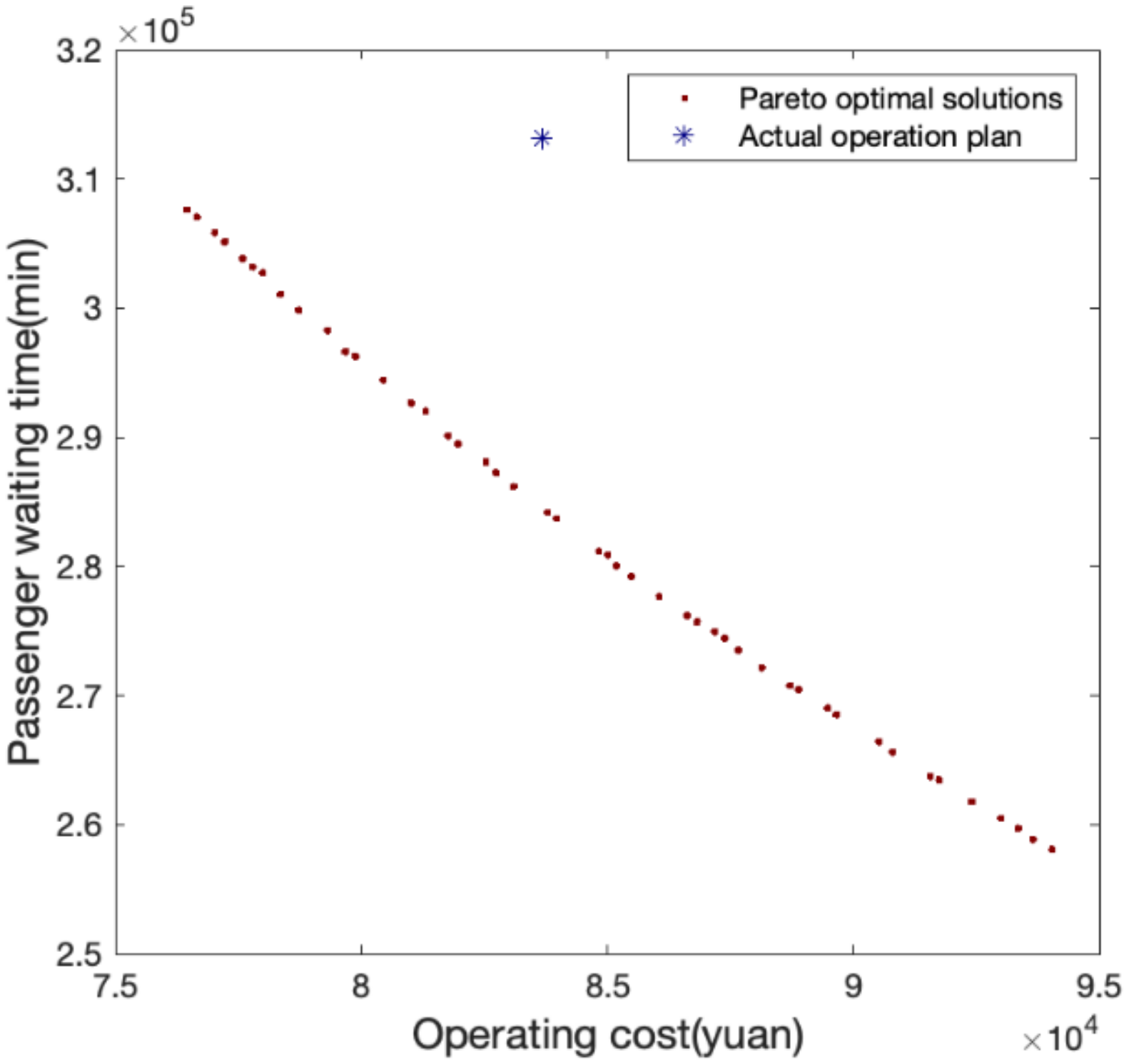
A case study of Chongqing, China, is carried out to analyze and verify the effectiveness and efficiency of the framework. The Pareto frontier solutions are provided to bus operators as alternative operation schemes.

2. Problem Description

In this section, we introduce the basic description of the M-TT/VS problem. We introduce the mathematical description of the multi-line operation mode and the processing methods of input data, including passenger flow data, trip runtime data, and other operational parameters. In addition, we construct the solution structure (i.e. output) for the M-TT/VS problem.

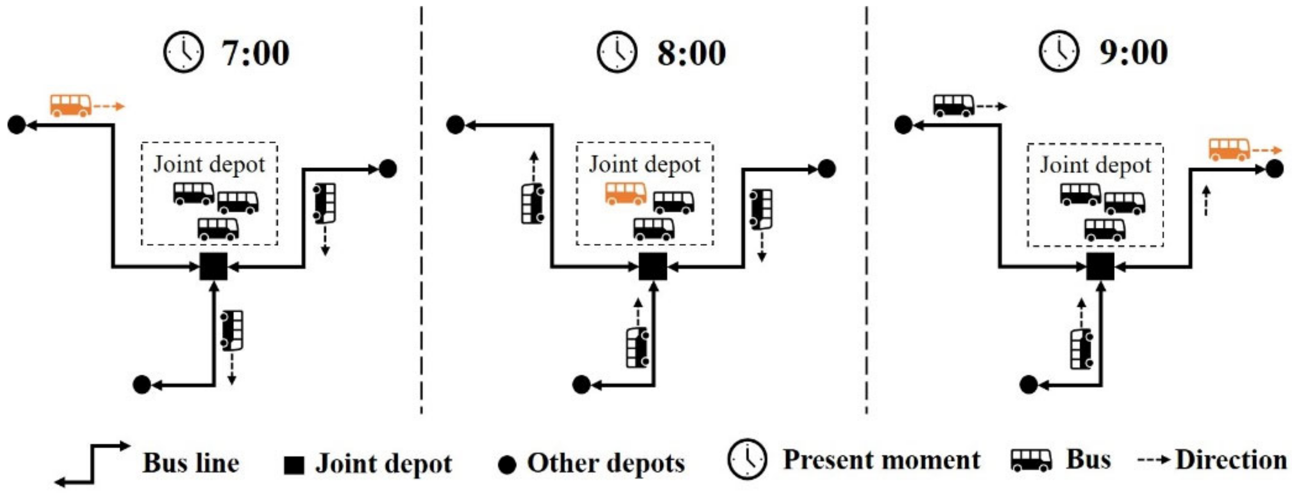
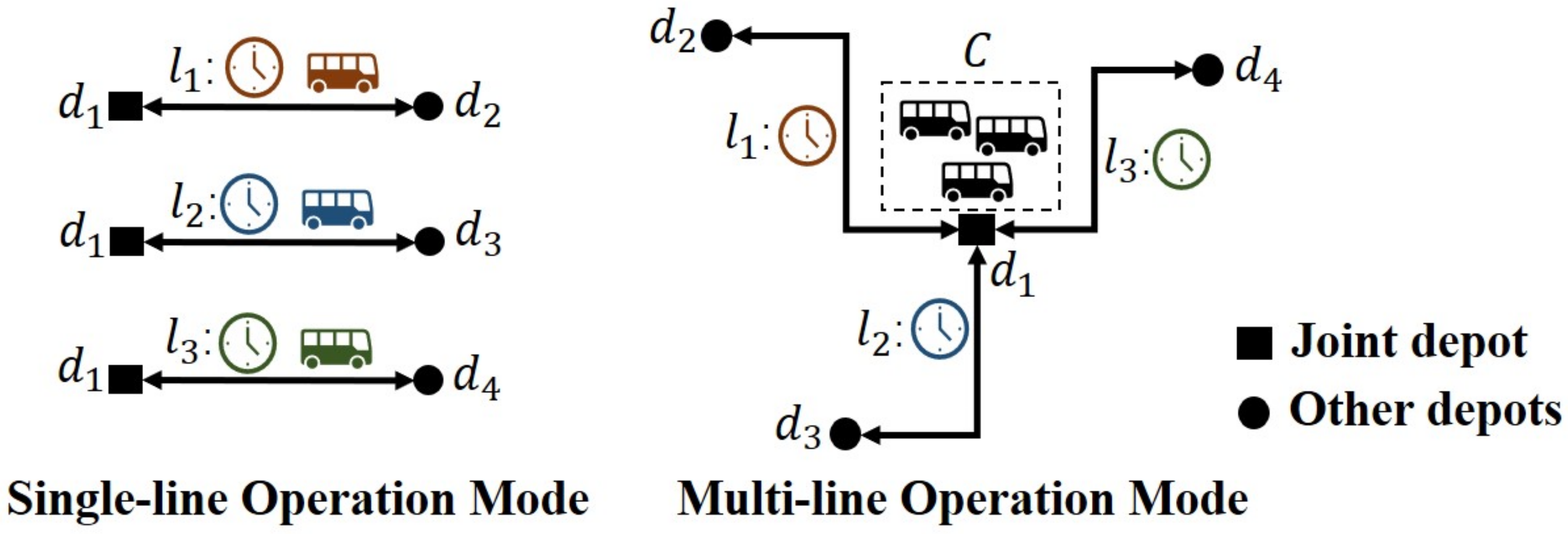
2.1. Description of the Multi-Line Operation Mode

The single-line operation mode and multi-line operation mode are two different operation modes, as described in Section 1. Figure 2 is a schematic diagram of different operation modes, taking three physical lines as an example. We use set $D=\left\{d_1,d_2,\dots ,d_{nd}\right\}$ to represent all the bus depots, and set $L=\left\{l_1,l_2,\dots ,l_{nl}\right\}$ to represent all the lines. Among set $L$, line $l_k$ contains three elements: starting depot $s{d}_k$, terminal depot $e{d}_k$, and operating mileage $m_k$ (represented as $l_k=\left\{s{d}_k,e{d}_k,m_k|l{s}_k,l{t}_k\in D\right\}).$ In the topology of Figure 2, these three lines have a joint depot $d_1$. Those vehicles used to operate these lines are defined as set $C=\left\{c_1,c_2,\dots ,c_{nc}\right\}$. In the single-line operation mode, vehicles are assigned to a specific line in advance and cannot shift during operation. In the multi-line operation mode, vehicles are centrally managed at the depot $d_1.$ That is, the vehicles can operate the plans among different lines. It should be noted that vehicles are not allowed to shift until they arrive at the joint depot.

2.2. Description of Input Data

Passenger flow data, trip runtime data, and operational parameters are known information for the M-TT/VS problem. They are key inputs for subsequent model solving. It should be noted that our research focuses on bus operation planning. We expect to find the rules of passenger flow and trip run time through historical data and design an operation scheme set with the rules. Therefore, we use the statistical and estimated data as input and evaluate the planning results based on the same data. The accuracy of subsequent implementation effect evaluation and data prediction is beyond the scope of this paper.

A brief introduction to them is given below.

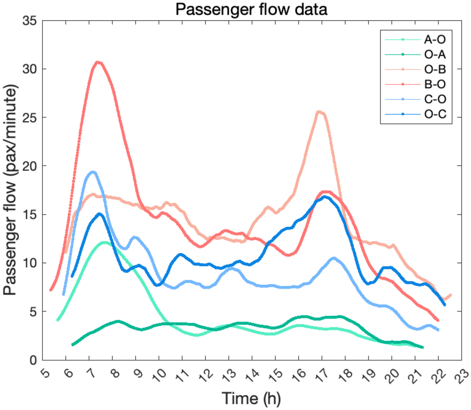
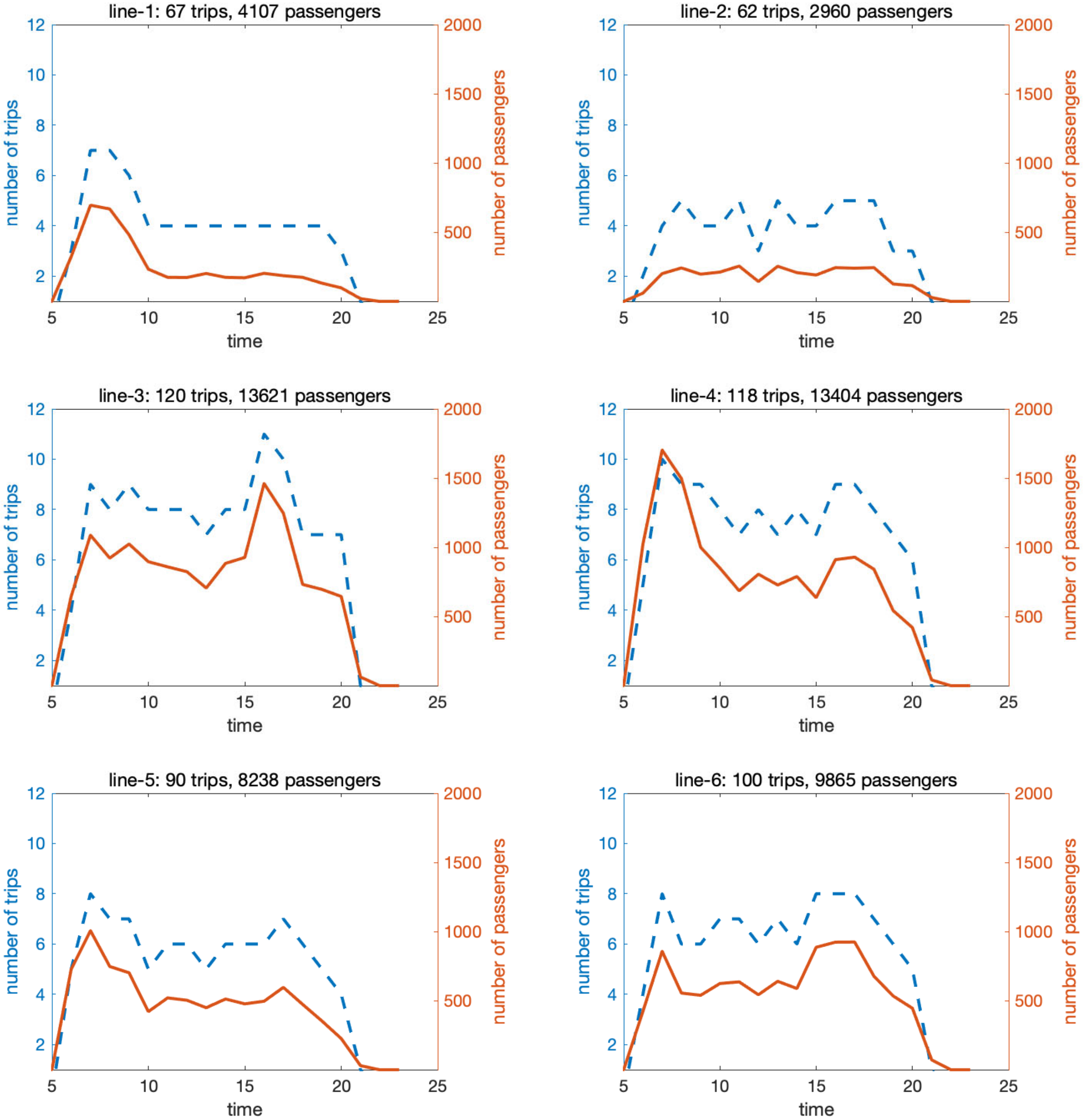
• Passenger flow data is obtained from historical IC card data. The IC card data enumerates passengers’ boarding times and trip numbers. At the same time, according to the operation data of vehicles, we can obtain the departure time and the line number of this trip. Therefore, we can count the total number of passengers carried on each trip. We assume that passengers are evenly distributed within the interval of two departure times. For example, suppose there is a trip carrying 100 passengers, and the departure time of this trip is 10 min apart from the previous trip. In this case, the arrival rate of passenger flow is 10 passengers/min. We have calculated the arrival rate of passenger flow $fn{p}_t^l$ of each line $l$ at time $t$. In addition, we restore the passenger’s alighting station data from IC card data through an alight inference method. Based on the complete passenger on-and-off action, we can calculate the highest section flow of the trips. The highest section flow of each line $l$ at time $t$ is represented as $fmn{p}_t^l$.

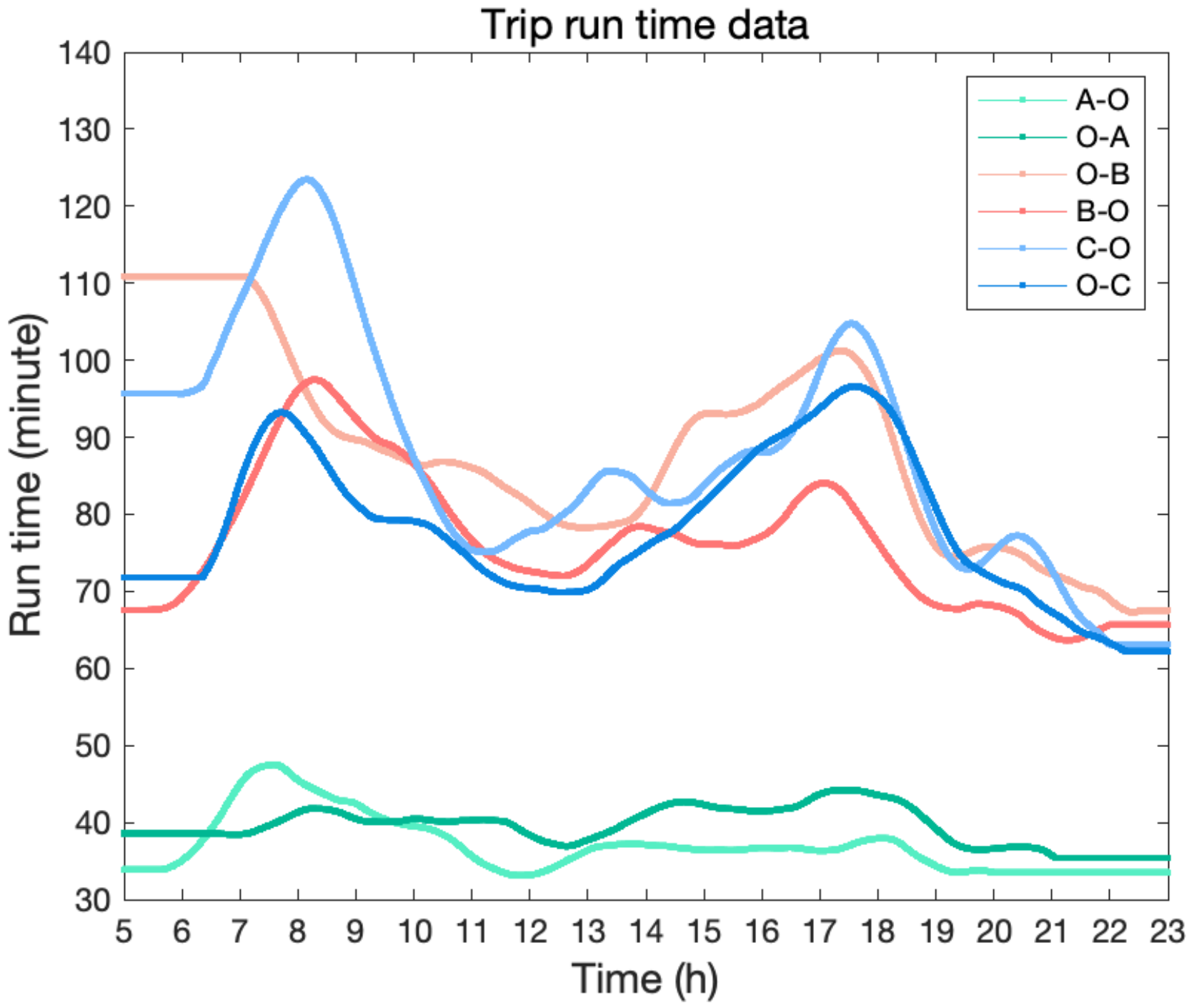
• Trip run time data is obtained from historical GPS data. For each line, we calculate the mean run time $fr{t}_t^l$ of the trips whose departure time is $t$ in a historical period. We also smooth the data and supplement the missing values, as shown in Equation (1).

$$fr{t}_t^l{}^{\prime }=\frac{1}{2\eta }·{\displaystyle \sum }_{x=t-\eta +1}^{t+\eta }fr{t}_x^l$$

(1)

• The operational parameters are determined based on actual operation scenarios. Part of these come from labor laws or regulations, and others from the experience of bus operators. The known operational parameters in this study include the set of all depots, set of all lines, number of standby vehicles, range of departure time, vehicle’s total operating time daily, minimum idle time between trips, and maximum departure time interval. These are listed in

  Table 1. Operational parameters.

  Parameters	Meaning
  $D$	Set of all depots
  $L$	Set of all lines
  $nc$	Number of vehicles
  $\left[s{t}_{min},s{t}_{max}\right]$	Range of departure time
  $\left[sr{t}_{min},sr{t}_{max}\right]$	Range of total operating time
  $it{a}_{min}$	Minimum idle time between trips
  $e{t}_{max}$	Maximum departure time interval

  .

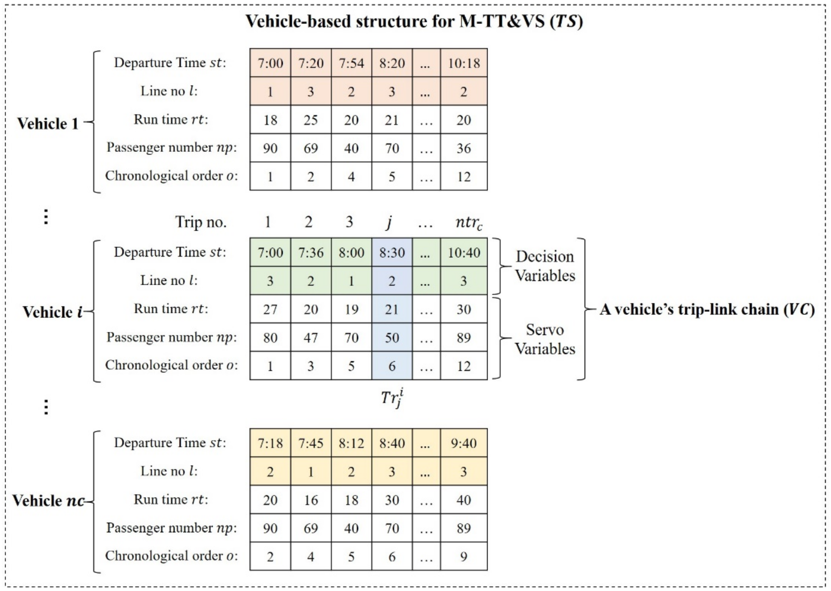
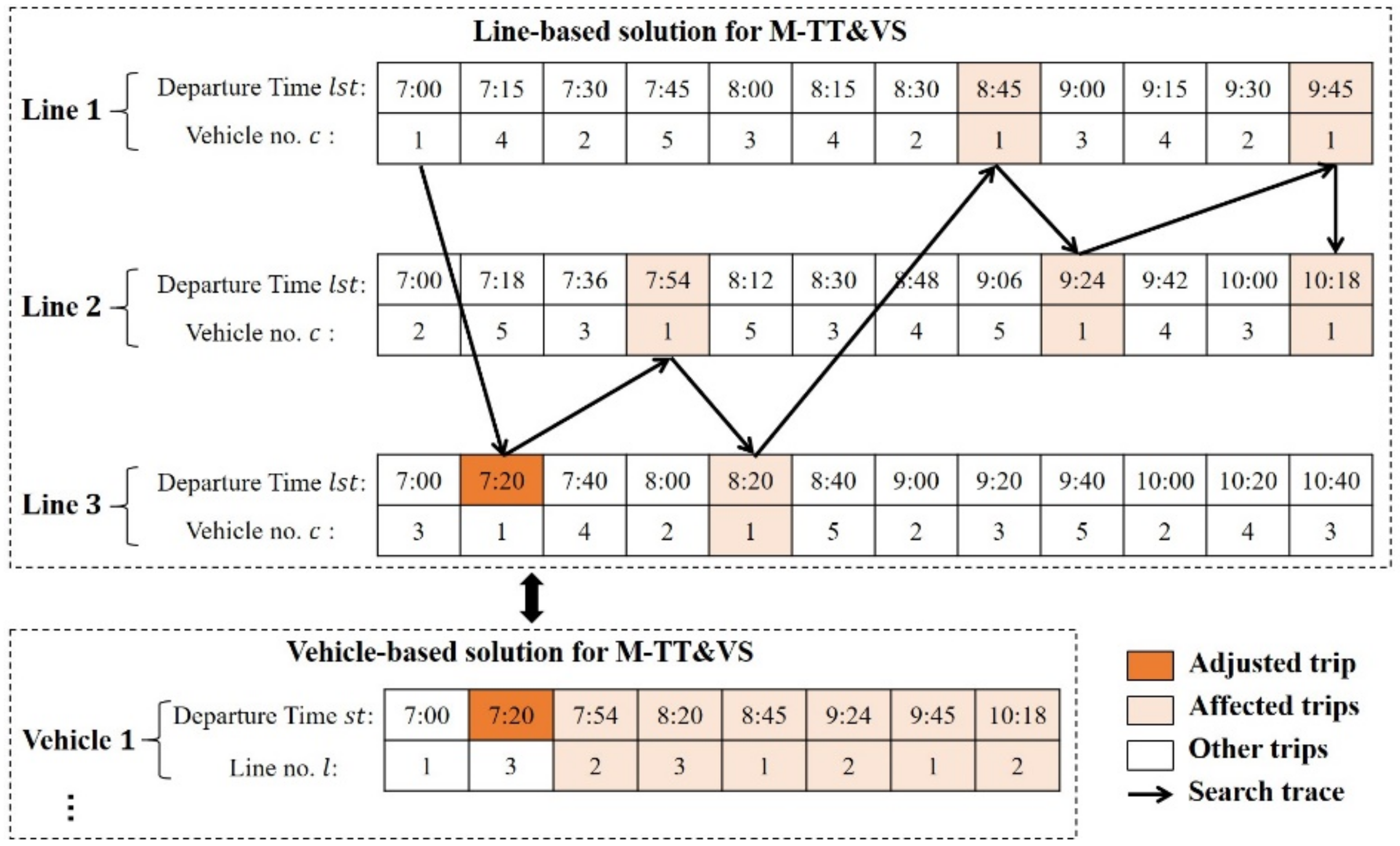
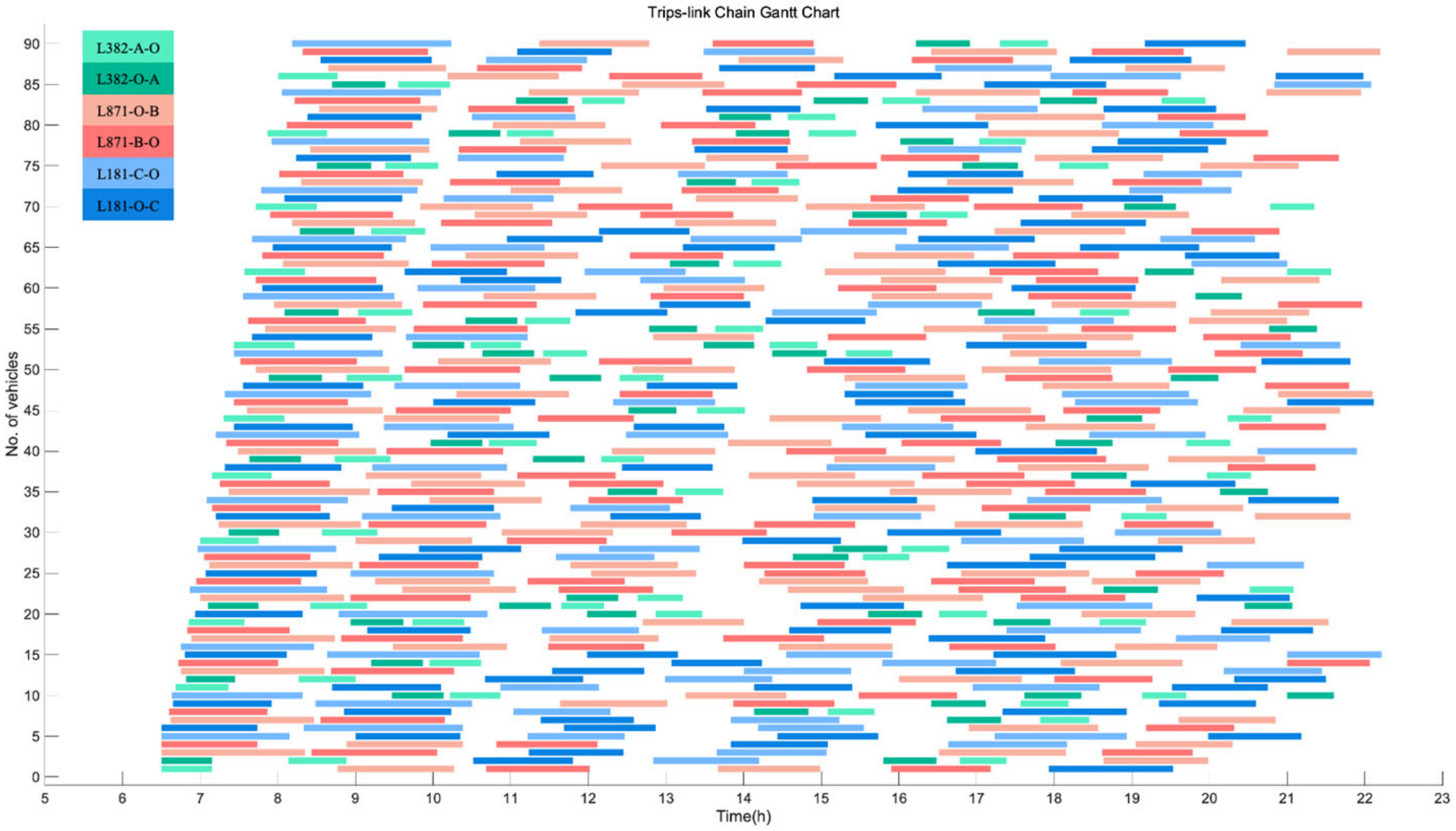
2.3. Solution Structure (Output)

As mentioned above, the departure times of trips and the vehicles of trips should be decision variables for the integration of TT and VS. We relate these two groups of decision variables by constructing the multiple vehicles’ trip-link chains with departure time information, as shown in Figure 3. A complete vehicle-based solution structure $TS$ contains multiple vehicles’ trip-link chains $VC$, represented as $TS=\left\{V{C}_1,V{C}_2,\dots ,V{C}_{nc}\right\}$. Every vehicle $i$ has a trip-link chain $V{C}_i$, which contains multiple chronologically ordered trips $Tr$, represented as $V{C}_i=\left\{T{r}_1^i,T{r}_2^i,\dots ,T{r}_{nt{r}_c}^i\right\}$. Both decision variables and servo variables can be included as elements in $Tr$.The $j$th trip of vehicle $i$ is represented as $T{r}_j^i=\left\{l_j^i,s{t}_j^i,r{t}_j^i,n{p}_j^i,o_j^i\right\}$, which is marked in light blue in Figure 3. Among them, the line numbers $l$ and the departure times $st$ are decision variables. The line numbers satisfies $l\in L$ unless $l=\varnothing$. The vehicles of trips are implicit in the structure as the indexes. Thus, an integrated solution that includes both TT decisions and VS decisions is organized. The servo variables include run time $rt$, passenger number $np$, and chronological order number $o$. $rt$ and $np$ are determined by the input data $fr{t}_t^l$ and $fn{p}_t^l$ (described in Section 2.2), which satisfy the Equations (2) and (3). Thus, a vehicle-based solution structure can be represented as $TS=\left\{\left(l_j^i,s{t}_j^i,r{t}_j^i,n{p}_j^i,o_j^i\right)|i\in \left\{1,2,\dots ,nc\right\}, j\in \left\{1,2,..,nt{r}_c\right\}\right\}$.

$$r{t}_j^i=fr{t}_{s{t}_j^i}^{l_j^i}$$

(2)

$$n{p}_j^i={\displaystyle \sum }_{z=ta}^{tb-1}fn{p}_z^{l_j^i} \left(ta=ls{t}_{o_j^i-1}^{l_j^i },tb=ls{t}_{o_j^i}^{l_j^i }\right)$$

(3)

$$\begin{array}{c}ls{t}_{o_j^i}^{l_j^i }=s{t}_j^i\end{array}$$

(4)

Compared with the line-based structure used in other typical papers [14,16], the vehicle-based structure can significantly reduce search complexity and improve optimization efficiency, because we can calculate and judge the performability of trips and availability of vehicles more directly with the vehicle-based structure, as shown in Figure 4. This will be explained in detail as follows.

In the optimization process, there are two indispensable and frequent processes: (1) judging whether the operation plan of each vehicle can be implemented; (2) assessing the feasible range for adjustment through two continuous trips of a vehicle. These processes are based on a sub-search process: for any trip $j$ of vehicle $i$, find the next trip $j+1$ of vehicle $i$. In the line-based structure, the lines’ trip-link includes the decision variables, represented as $L{C}_k=\left\{\left(ls{t}_j^k,c_j^k\right)| j\in \left\{1,2,..,nt{r}_l\right\}\right\}$ for the single line $k$. A complete line-based solution structure $LS$ contains multiple lines’ trip-link chains $LC$. We should do additional searches and calculations for the sub-search process with this line-based structure, as shown in

Table 2. The sub-search process with the line-based structure.

$\mathbf{Task}: \mathbf{Find} \mathbf{the} \mathit{j}+1$$\mathbf{Trip} \mathbf{of} \mathbf{Vehicle} \mathit{i}$		Time Complexity
1	$\mathrm{For} k\in \left\{1,2,\dots ,nl\right\}$$, \mathrm{Find} xL{C}_k=\left\{\left(ls{t}_m^k,c_m^k\right)| \left(ls{t}_m^k,c_m^k\right)\in L{C}_k and c_m^k=i\right\}$;	$O\left(nl\times nt{r}_l\right)$
2	For $c=i$, Get union set $yLC={\mathrm{U}}_{k=1}^{nl}xL{C}_k$;	$O\left(nl\right)$
3	$\mathrm{Sort} yLC$$, \mathrm{Get} zLC=\left\{\left(s{t}_j,i\right)| \left(s{t}_j,i\right)\in yLC and s{t}_{j+1}>s{t}_j,\forall j>1\right\}$;	$O\left(nt{r}_c\times nt{r}_c\right)$
4	$\mathrm{Get} s{t}_{j+1}$	$O\left(1\right)$

. The time complexity with the line-based structure is estimated to be $O\left(nl\times nt{r}_l+nl+nt{r}_c\times nt{r}_c\right)$ for a sub-search task. But in the vehicle-based structure, we can get the next trip $T{r}_{j+1}^i$ directly by indexing with time complexity $O\left(1\right)$. Obviously, the use of a line-based structure will cause a significant time cost in the optimization process, especially in the multi-line operation mode. Because the search task’s time complexity, the line-based structure increases with the number of lines $nl$. Therefore, we use the vehicle-based structure to improve search and calculation efficiency in the optimization process. Of course, after the optimization process, the vehicle-based solution can be re-organized as the line-based solution.

3. Methodology

This section constructs a multi-objective optimization model and a heuristic solution algorithm for the M-TT/VS problem. The optimization model considers higher service quality and lower operating costs as objectives. Logic and operational rules are considered as constraints. A heuristic solution algorithm is designed to find the Pareto frontier solutions, which are provided to bus operators as alternative operation schemes.

3.1. Optimization Model

The primary trade-off faced in bus service planning is between the level of service faced by the passengers and the operating costs for agencies [5,22]. The improvement of service quality requires higher operating costs, and the reduction of operating costs will always affect the service quality. Owing to the existence of different business models, there is no unified standard to balance the two goals. It isn’t easy to quantify the weights of the two goals. Therefore, we establish a multi-objective optimization model to systematically optimize these two goals. The objective function is expressed in Equations (5) and (7). The objective function $Z_1$ represents the total waiting time of passengers. As a basic transport service, operating rules usually specify the maximum departure time interval. We assume that the maximum waiting time that passengers can tolerate is larger than the maximum departure time interval. Therefore, the total waiting time of passengers can represent the service quality. The objective function $Z_2$ represents the operating cost, which is calculated by multiplying the operating cost per kilometer by the total operating kilometers.

$$\min Z=\left(Z_1,Z_2\right)$$

(5)

$$Z_1={\displaystyle \sum }_{i=1}^{nl}{\displaystyle \sum }_{j=1}^{nt{r}_l-1}{{\displaystyle \sum }}_{z=ls{t}_j^l}^{ls{t}_{j+1}^i-1}fn{p}_z^i·\left(ls{t}_{j+1}^i-z\right)$$

(6)

$$Z_2=C_m·{\displaystyle \sum }_{i=1}^{nc}{\displaystyle \sum }_{j=1}^{nt{r}_c}{m}_j^i$$

(7)

Solutions are also required to be constrained by logic and operating rules. The constraints are expressed in Equations (8)–(16). Equation (8) specifies that the departure time $s{t}_j^i$ is an integer. That is, the departure time is a minute node. Equation (9) stipulates that the departure time $s{t}_j^i$ is within the specified range, which represents the bus operation period of the day. In the other case, if the $j$th trip of vehicle $i$ is not scheduled, the departure time $s{t}_j^i$ is marked as 0. Equation (10) stipulates that the departure time interval is not greater than the specified value. Equations (11) and (12) stipulate that the first departure time and the last departure time of each line are given values, which are consistent with Equation (9). Equation (13) stipulates that the idle time between two connected trips of each vehicle is not less than the given value. Equation (14) stipulates the preceding arrival station be the same as the subsequent departure station. That is, deadhead is not allowed. Equation (15) stipulates the total operating time of each vehicle within a given range. The on-and-off behavior of passengers results in the accumulation of passenger flow at sections. Formula (16) guarantees that the maximum section flow is not greater than the maximum seating capacity of the vehicle.

$$s{t}_j^i\in \mathbb{Z} ,\left(i=1,2,\dots ,nc;j=1,2,\dots ,nt{r}_c\right)$$

(8)

$$t_{min}\le s{t}_j^i\le t_{max} or s{t}_j^i=0,\left(i=1,2,\dots ,nc;j=1,2,\dots ,nt{r}_c\right)$$

(9)

$$ls{t}_{j+1}^i-ls{t}_j^i\le e{t}_{max},\left(i=1,2,\dots ,nl;j=1,2,\dots ,nt{r}_l\right)$$

(10)

$$ls{t}_1^i=t_{min},\left(i=1,2,\dots ,nl\right)$$

(11)

$$ls{t}_{\max \left(o^i\right)}^i=t_{max},\left(i=1,2,\dots ,nl\right)$$

(12)

$$s{t}_{j+1}^i-\left(r{t}_j^i+s{t}_j^i\right)\ge it{a}_{min},\left(i=1,2,\dots ,nc;j=1,2,\dots ,nt{r}_c-1\right)$$

(13)

$$e{d}_j^i=s{d}_{j+1}^i, \left(i=1,2,\dots ,nc;j=1,2,\dots ,nt{r}_c-1\right)$$

(14)

$$sr{t}_{min}\le {\displaystyle \sum }_{j=1}^{nt{r}_c}r{t}_j^i\le sr{t}_{max}\left(i=1,2,\dots ,nc\right)$$

(15)

$$mn{p}_j^i\le C{S}_{max} \left(i=1,2,\dots ,nc;j=1,2,\dots ,nt{r}_c-1\right)$$

(16)

which:

$$mn{p}_j^i={\displaystyle \sum }_{z=ta}^{tb-1}fmn{p}_z^{l_j^i} \left(ta=ls{t}_{o_j^i-1}^{l_j^i },tb=ls{t}_{o_j^i}^{l_j^i }\right)$$

(17)

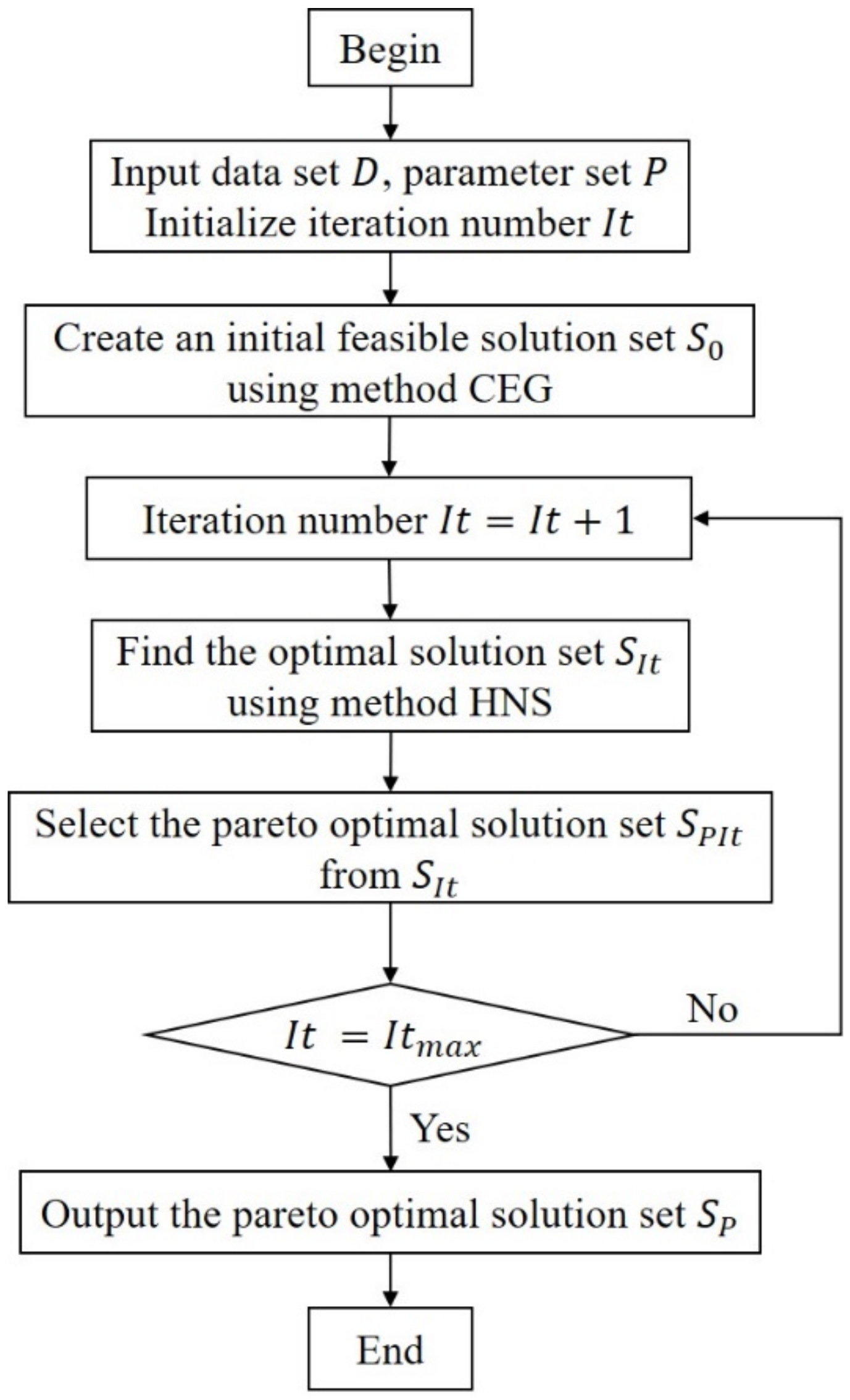
3.2. Solution Algorithm

The M-TT/VS problem to be solved in this study is complex. It requires a lot of time to solve the problem accurately. Therefore, we propose a heuristic method. As mentioned above, the solution structure is a vehicle-based structure $TS$, where $l_j^i$ and $s{t}_j^i$ are decision variables. Namely, we need to determine each trip’s operation line and departure time. Our goal is to find the Pareto frontier solutions under the multi-objective model. Therefore, we design a feasible solution generation algorithm based on greedy rules (CEG), an optimization algorithm based on neighborhood search (HNS), and a method to screen the Pareto frontier solutions. The algorithm flowchart is shown in Figure 5.

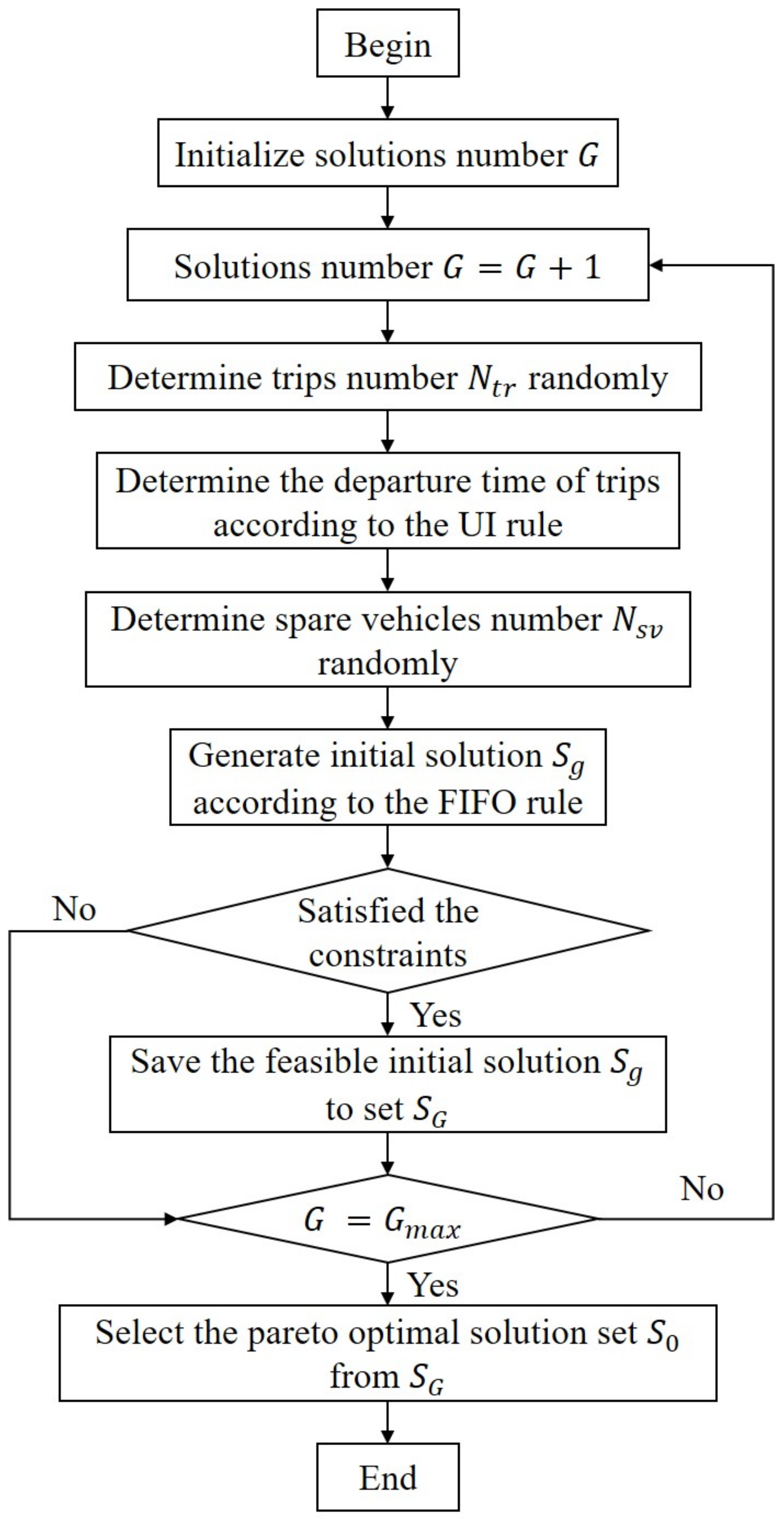
3.2.1. Phase 1: Generate Feasible Solutions

A real feasible solution needs to meet complex operational constraints. If there is no intervention in the solution process, it will cause the continuous generation of invalid solutions. Further, this will result in a waste of solving resources and the reduction of solving efficiency. Therefore, we design an efficient feasible solution generation algorithm CEG.

The CEG algorithm flowchart is shown in Figure 6. The departure time of trips is determined by the randomly generated number of trips and the uniform interval rule (UI). The UI rule is a greedy rule, which ignores the change of passenger flow and requires the departure interval to be consistent [17,23]. Since constraints (11) and (12) specify the first and last departure times, we can determine the unique departure interval by dividing the number of trips by the length of the operating period. Thus, the minimum value of the number of trips on each line can be specified to satisfy the constraint (10). Then, the entire trip-link chain group is determined based on departure time and the first in, first out rule (FIFO). The FIFO rule is a greedy selection rule when multiple vehicles are scheduled. Early arrivals are always selected first [6]. We randomly determine the first trips of vehicles, then traverse the remaining trips in chronological order, and assign them to the trip-link chain according to the FIFO rule. For the generated initial solution, we judge whether it meets all constraints. Finally, the Pareto frontier solution is selected by pairwise comparison of feasible solutions.

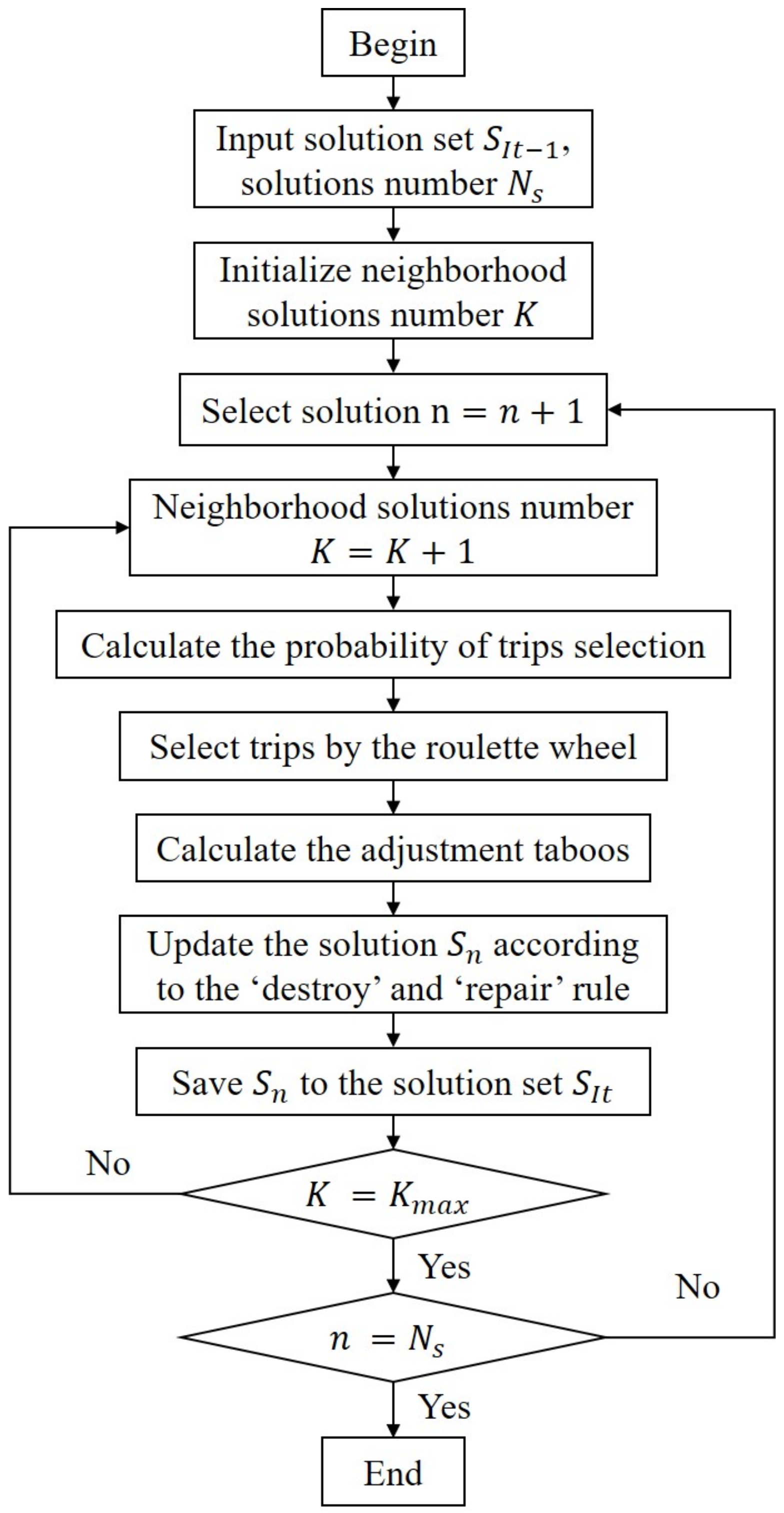
3.2.2. Phase 2: Optimize Solutions

The neighborhood search algorithm is a typical local search algorithm [24]. The design of neighborhood search rules is flexible and can be easily combined with heuristic information related to the problem. Therefore, to optimize the M-TT/VS problem, we design a heuristic optimization algorithm based on the neighborhood search algorithm HNS.

The HNS algorithm flowchart is shown in Figure 7. The differences in heuristic search algorithms are mainly reflected in the search rules. For example, a genetic algorithm generates candidate solutions by crossover and mutation, while a neighborhood search algorithm produces candidate solutions by detriment and repairment. We designed the “destroy” rule and “repair” rule. The “destroy” rule refers to the rule of selecting decision variables that need to be changed in a solution. We fused heuristic information $c{p}_j^i$ to guide the selection probability. Heuristic information $c{p}_j^i$ refers to the difference between the passenger number of trip carries and the base value. The more significant the difference is, the more likely it is to be selected. A roulette wheel is used to choose the target trip $T{r}_j^i$. We define those similar trips near the target trip as needing change. For example, suppose the trip $T{r}_j^i$ carries more than the base value. In that case, the trips $[k_j^i-R,k_j^i+R]$ of line $l_j^i$, which also carries more than the base value, are the similar trips. The “repair” rule refers to the method of trip adjustment. For trips that need to be adjusted, we designed a comprehensive tabu table, requiring trips to be adjusted without breaking constraints. In addition, we require trip adjustment in line with practical experience limitations. If the number of passengers on a trip exceeds the baseline, we will adjust the departure interval as little as possible. The heuristic information and the comprehensive tabu table are described in detail below.

Heuristicinformation$c{p}_j^i$. Based on practical operational experience, service supply should conform to changes in demand. If the number of passengers on a trip exceeds the baseline, our optimization direction should reduce the number. The specific operation method is to reduce the departure interval, which means we should push forward the departure time of the next trip in the same direction and vice versa. Based on this idea, we propose heuristic information $c{p}_j^i$. The numerical value of $c{d}_i^j$ provides the probability the trip will be destroyed, and $c{p}_i^j$ plus or minus tells us how to adjust trips.

$$c{p}_j^i=n{p}_j^i-\overline{n{p}_{l_j^i}}$$

(18)

$$c{d}_j^i=\left|c{p}_j^i\right|$$

(19)

Comprehensivetabu table. In the optimization process, it is essential to ensure the feasibility of the solution, especially when there are many external constraints. We construct a comprehensive tabu table to confirm the validity of our solution. We can adjust solutions to the extent that the constraints allow. These constraints can be divided into two categories: (a) in the same line $l_j^i$ of the target $T{r}_j^i$, the forward and backward adjustment should be within a specific range to avoid repeated departure times and unreasonable departure intervals; (b) in the same vehicle $j$ of the target $T{r}_j^i$, the connection between $T{r}_j^{i-1}$, $T{r}_j^i$ and $T{r}_j^{i+1}$ also limits the range of adjustment to avoid conflicting vehicle arrangements. $ct{t}_l^{i,j}$ and $ct{t}_r^{i,j}$ are the boundaries where $s{t}_i^j$ can be adjusted forward and backward, respectively.

$$ct{t}_l^{i,j}=\max \left(t_{min},ls{t}_{o_j^i-1}^{l_j^i }, s{t}_j^{i-1}+r{t}_j^{i-1}+it{a}_{min}\right)$$

(20)

$$ct{t}_r^{i,j}=\min \left(t_{max},ls{t}_{o_j^i+1}^{l_j^i }, s{t}_j^{i+1}-it{a}_{min}-r{t}_j^i\right)$$

(21)

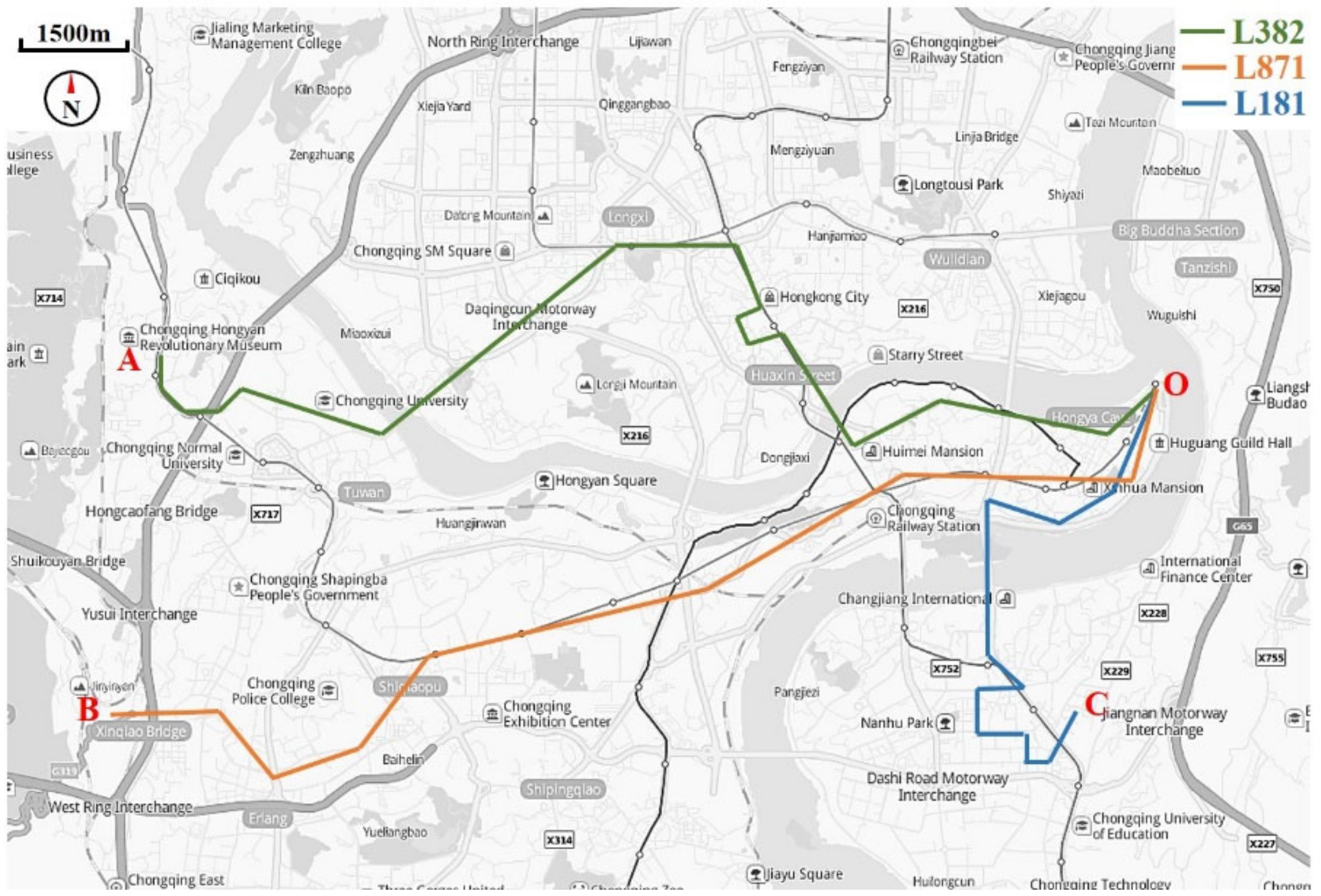
4. Case Study and Discussion

This section verifies the effectiveness of the multi-objective integrated framework through practical cases. We verify that the algorithm can solve the Pareto frontier effectively, and prove the advantages of the algorithm through comparative experiments. Finally, we also compare the difference of operation service schemes that can be provided under different operation modes with the same number of vehicles.

4.1. Case Description and Data Preparation

To verify the effectiveness of the model and algorithm above, a typical multi-line scenario is taken as the case. The case is in Chongqing, China, and contains four depots and three lines, as shown in Figure 8. The four depots are represented by A, B, C, and O. The three lines are line 382, 871, and 181, and they all contain the upstream and downstream directions. The depot O is a hub where vehicles can be centrally scheduled.Thus the depots and lines form a typical multi-line operation mode.

Passenger flow data and trip run time data are the main input data of this study. Based on the IC card data and vehicle GPS data of Chongqing in June 2020, we figure out which trip the passenger was on and when the trip departed. About 780 trips are operated and around 55,000 passengers are recorded per day. Through data cleaning, calculating, and smooth processing (as mentioned in Section 2.2), the final input data $fnp$ and $frt$ are obtained, as shown in Figure 9 and Figure 10.

The values of parameters are set according to the actual operation requirements, and they are listed in

Table 3. The values of parameters.

Parameters	Meaning	Value
$D$	Set of all depots	$\left[A,B,C,O\right]$
$L$	Set of all lines	$\left\{\begin{array}{c}\left(A,O,9.5 \mathrm{km}\right)\\ \left(O,A,9.5 \mathrm{km}\right)\\ \left(O,B,18 \mathrm{km}\right)\\ \left(B,O,18 \mathrm{km}\right)\\ \left(C,O,20.5 \mathrm{km}\right)\\ \left(O,C,20.5 \mathrm{km}\right)\end{array}\right\}$
$nc$	Number of vehicles	90
$\left[t_{min},t_{max}\right]$	Range of departure time	[6:30,21:00]
$\left[sr{t}_{min},sr{t}_{max}\right]$	Range of total operating time	[4 h,15 h]
$it{a}_{min}$	Minimum idle time between trips	5 min
$e{t}_{max}$	Maximum departure time interval	20 min
$C{S}_{max}$	Maximum seating capacity	90 seats
$C_m$	Operating cost per kilometer	10 yuan/km

.

4.2. Results and Discussion

By using the multi-objective optimization model and heuristic solution algorithm method proposed before, we try to solve the above cases. MATLAB version R2021b is used, run on a computer with macOS Monterey, Intel Core I9, and 32GB random access memory.

4.2.1. Description of Results

The number of initial solution sets is set as 100, and the number of optimization iterations is set as 500. We get 46 Pareto frontier solutions when the computation time is less than 15 min. All the solutions satisfy the constraint. Figure 11 shows the objective function value distribution of the Pareto frontier solutions. These solutions are all better than the actual operational plan.

We use Euclidean distance to express the effect of Pareto frontier solutions in each iteration. The calculation is shown in Equation (22). The smaller the Euclidean distance, the closer the position of the solution is to the origin. Figure 12 shows how minimum Euclidean distance changes with the number of iterations. The results eventually tend to converge.

$$E_{it}^s=\sqrt{{\left(\frac{Z_1^s}{10000}-0\right)}^2+{\left(\frac{Z_2^s}{1000}-0\right)}^2}$$

(22)

Figure 13 shows a solution in the Pareto frontier solutions. A row represents a trip-link chain, and a panel represents a trip. The number before the “−” is a line number, and the number following the “−” is a departure time (minute timestamp). The object function value (passenger waiting time) is 25,8084 min and the operating cost is CNY 94,045. All operational constraints are met.

For Solution-A, the optimized objective function value of passenger waiting time is 25,8084 min, and the total passenger number is 52,195. We map the passenger waiting time as a histogram distribution in Figure 14. It can be seen that the waiting time of most passengers is less than 5 min, and the number of passengers waiting for five to twenty minutes gradually decreases.

Our solution ensures that supply and demand are matched not only on different routes but also over different time periods, as shown in Figure 15. As we can see, the more passengers on the line/time, the higher the heat, the more trips supplied.

The Gantt diagram corresponding to this solution is shown in Figure 16. The diagram provides a visual representation of Solution-A and clearly shows the vehicle’s daily operation schedule. As can be seen from the color transformation, vehicles can shift between multiple lines.

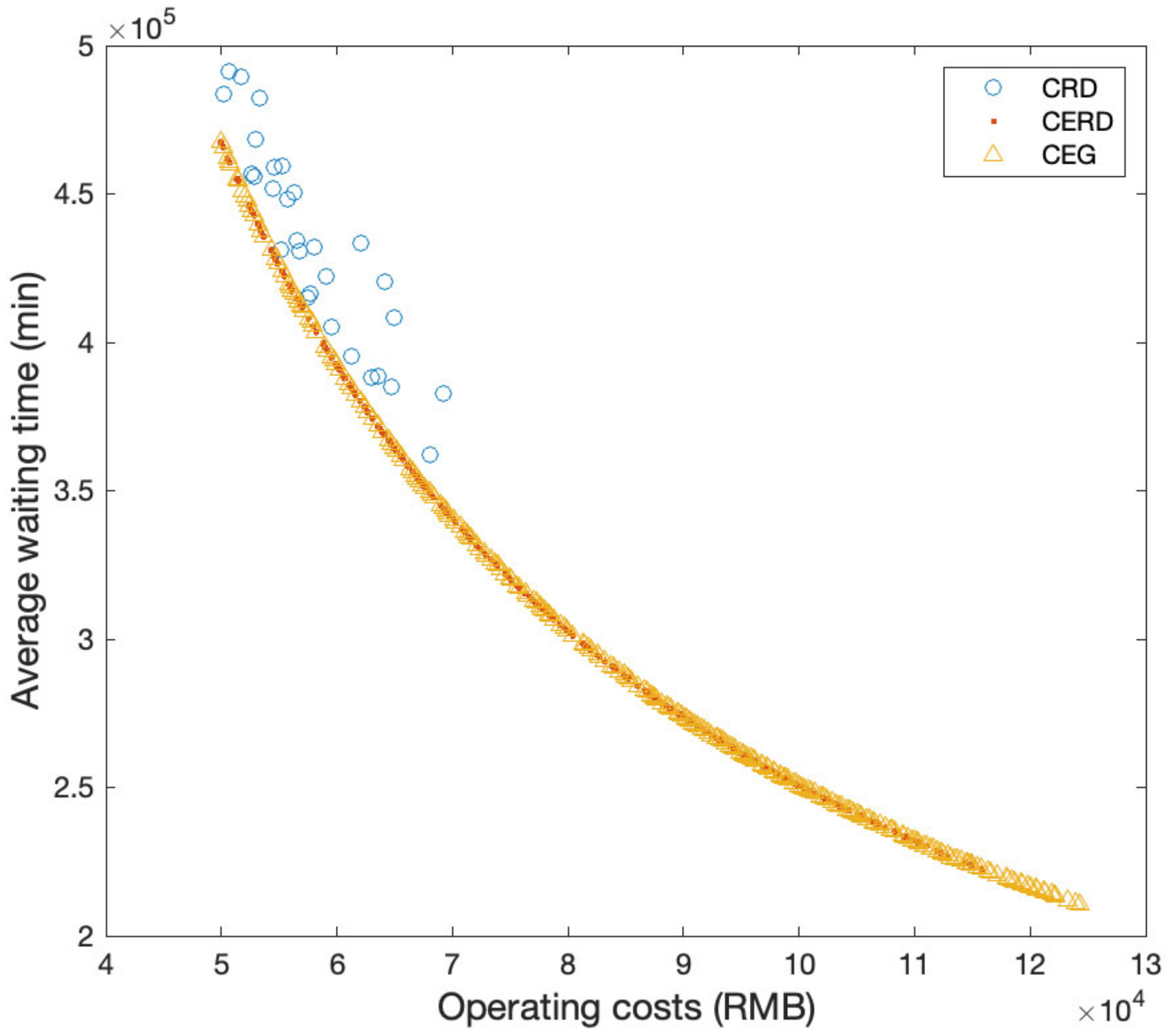
4.2.2. Contrast Experiment of Generation Algorithm

A feasible solution generation algorithm CEG is proposed in Section 3.2. CEG requires vehicle scheduling compliance with the FIFO rules and timetabling compliance with UI rules. To verify the coverage of feasible solutions’ objective function value and the efficiency of generating feasible solutions, we compare CEG with commonly used algorithms: random algorithm (CRD) and partly greedy algorithm (CERD). CRD is completely random, scheduling vehicles randomly based on the random frequency in each period. CERD is partly random, scheduling vehicles randomly but timetabling in compliance with UI rules. Basic logical rules are considered in these algorithms.

We changed the total number of solutions $G_{max}$, and did six comparative experiments. The feasible solution generation efficiencies by different algorithms are shown in

Table 4. The feasible solution generation efficiencies by different algorithms.

No.	${\mathit{N}}_{\mathit{s}}$	CRD		CERD		CEG
		${\mathit{N}}_{\mathit{e}\mathit{s}}$	${\mathit{P}}_{\mathit{e}\mathit{s}}$	${\mathit{N}}_{\mathit{e}\mathit{s}}$	${\mathit{P}}_{\mathit{e}\mathit{s}}$	${\mathit{N}}_{\mathit{e}\mathit{s}}$	${\mathit{P}}_{\mathit{e}\mathit{s}}$
1	500	17	3%	267	53%	332	66%
2	700	33	5%	370	53%	447	64%
3	1000	51	5%	498	50%	646	65%
4	1500	49	3%	765	51%	1007	67%
5	2000	77	4%	978	49%	1292	65%
6	3000	100	3%	1481	49%	1987	66%

. The number of feasible solutions is recorded as $N_{es}$ and the proportion of feasible solutions is recorded as $P_{es}$. It can be seen from the results that the efficiency of CRD is the lowest, at less than 4%. CERD shows a big improvement in efficiency, of above 50%. CEG has the highest efficiency of 65%, which is 15% higher than CERD. We also compare the range of the objective function values by different algorithms. The results are shown in

Table 5. The range of the objective function values by different algorithms.

No.	${\mathit{N}}_{\mathit{s}}$	CRD		CERD		CEG
		$\mathit{R}\mathit{O}\mathit{C}\times {10}^4$	$\mathit{R}\mathit{W}\mathit{T}\times {10}^5$	$\mathit{R}\mathit{O}\mathit{C}\times {10}^4$	$\mathit{R}\mathit{W}\mathit{T}\times {10}^5$	$\mathit{R}\mathit{O}\mathit{C}\times {10}^4$	$\mathit{R}\mathit{W}\mathit{T}\times {10}^5$
1	500	[5.08,7.18]	[3.68,4.78]	[5.05,11.23]	[2.28,4.62]	[5.07,12.43]	[2.11,4.61]
2	700	[5.06,7.02]	[3.56,4.81]	[4.99,11.25]	[2.28,4.67]	[5.01,12.33]	[2.12,4.66]
3	1000	[5.10,7.14]	[3.65,4.84]	[4.99,11.54]	[2.23,4.67]	[4.99,12.22]	[2.13,4.67]
4	1500	[5.09,8.66]	[3.06,4.72]	[4.99,11.66]	[2.21,4.67]	[4.99,12.43]	[2.11,4.67]
5	2000	[5.12,8.01]	[3.46,4.85]	[4.99,11.92]	[2.18,4.67]	[4.99,12.43]	[2.11,4.67]
6	3000	[4.99,7.91]	[3.25,5.02]	[4.99,11.54]	[2.23,4.67]	[4.99,12.43]	[2.11,4.67]

, where $ROC$ represents the range of operating costs and $RWT$ represents the range of passenger waiting time. Figure 17 shows the result of objective function values when $G_{max}=1000$. Obviously, the $ROC$ and $RWT$ of CEG is the broadest. CEG and CERD have a greater improvement in $ROC$ and $RWT$ compared with CRD. It should be mentioned that CEG and CERD can find more low-passenger-waiting-time solutions, which is meaningful for the operation enterprises pursuing service quality. In general, CEG not only has higher $P_{es}$, but also has broader $ROC$ and $RWT$.

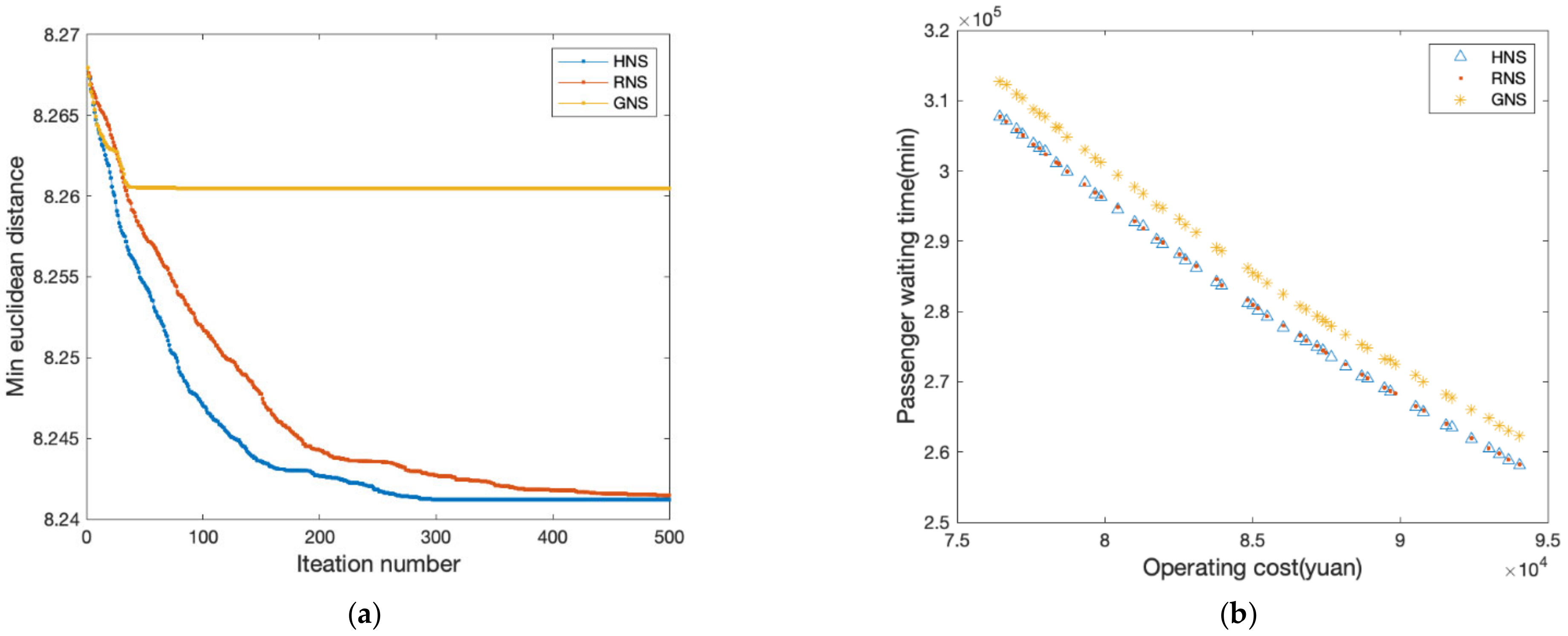
4.2.3. Contrast Experiment of Optimization Algorithm

An optimization algorithm based on neighborhood search HNS is proposed in Section 3.2. Special neighborhood search rules are designed to solve the problem. We compare heuristic neighborhood algorithm HNS with the random neighborhood algorithm (RNS) and greedy neighborhood algorithm (GNS) in optimization efficiency and solution quality through experiments. The three algorithms differ in their “destroy” and “repair” rules. RNS has random “destroy” and “repair” rules without using heuristic information, while GNS has greedy “destroy” and “repair” rules using the same heuristic information as HNS.

We kept the initial solution consistent and conducted a comparative experiment. Figure 18a shows the iterative optimization effects of the three algorithms, and Figure 18b shows the distribution of the final solution set of the three algorithms. It is obvious that GNS easily falls into local optimum, and the result of the final solution set is obviously worse than the other two methods. The final solution set distribution of RNS and HNS is similar, but the optimization efficiency of RNS is inferior to HNS. In general, HNS improves the optimization efficiency on the condition that the quality of the final solution set is guaranteed.

In order to compare the solutions’ differences through these three algorithms, we draw operating cost distribution and the passenger waiting time distribution of the Pareto frontier solution set, respectively. The distributions of operating costs are similar, consistent with Figure 19a. It can be seen from Figure 19b that the HNS and RNS have less high-waiting-time solutions.

In addition, we compared the matching degree of supply and demand under the same line and different trips, as shown in Figure 20. It can be seen that the supply of each period is in line with the demand, although the total supply is different. Therefore, solutions in the Pareto frontier are meaningful and can be selected by bus operation managers according to their needs.

4.2.4. Contrast Experiment of Operation Mode

As mentioned above, the multi-line mode saves resources because vehicles are centrally scheduled at hubs. We verify this by comparing the results in different operation modes. Figure 21a,b respectively show the minimum passenger waiting time and maximum operating cost that can be achieved in different modes, i.e., the best service and maximum supply that can be achieved in different modes. They vary with vehicle number. With the same number of vehicles, the multi-line operation mode can always achieve better service and provide more supply. In other words, the multi-line operation mode can achieve the same effect as the single-line operation mode with fewer vehicles.

4.2.5. Robustness Test

For a robustness test, we conduct a series of experiments towards the peak run time (7:00–8:00) fluctuated by 1% to 20% keeping the number of vehicles and operating costs constant. The optimization results are shown in the Figure 22. From the results, we evaluate that when the disturbance is less than 5% in the peak period, the model is still robust. When the disturbance is greater than 5%, the optimization results begin to be affected. When the disturbance reaches 20%, it is reduced by 0.125% compared with the result without perturbation.

5. Conclusions

This paper presents an integrated framework for timetabling and vehicle scheduling in multi-line operation mode. A vehicle-based solution structure constructing the multiple vehicles’ trip-link chains with departure time information is established to facilitate simultaneous optimization. The departure time can be adjusted in minutes freely to accommodate fluctuating demand. And we propose a multi-objective optimization model considering the actual operation constraints, such as the number of vehicles and the range of vehicle total operating time. The multi-objective optimization model considers higher service quality and lower operating costs as objectives. In addition, we design a heuristic algorithm for this model, which contains a feasible solution generation algorithm based on greedy rules and an optimization algorithm based on neighborhood search. CEG can generate feasible solutions on a large scale and efficiently. HNS accelerates the optimization through heuristic operators and tabu tables.

A case study of Chongqing, China is carried out to analyze and verify the effectiveness and efficiency of the framework. Results show that the Pareto frontier solutions can be obtained by this framework. Using the CEG algorithm, the ratio of effective solutions can reach 65%, and the coverage range of the objective function value is more extensive than other methods. The optimization efficiency and results of the HNS algorithm are better than other methods. Finally, we compare the extreme utility of the multi-line operation mode and the single-line operation mode. The multi-line operation mode can consistently achieve better service and supply when using the same number of vehicles.

Several opportunities for future research exist, such as further integration of driver scheduling and TT&VS, because driver salary costs are also essential for bus operations. It is also challenging to consider the constraints associated with drivers’ driving rules. In addition, M-TT/VS is also practical for use in emergencies, as occasional congestion or vehicle damage conditions prevent vehicles from running as planned.

References

1. Xinchao, Z.; Hao, S.; Juan, L.; Zhiyu, L. DP-TABU: An algorithm to solve single-depot multi-line vehicle scheduling problem. Complex Intell. Syst. 2021, 1–11. [Google Scholar] [CrossRef]
2. Petit, A.; Lei, C.; Ouyang, Y. Multiline bus bunching control via vehicle substitution. Transp. Res. Part B Methodol. 2019, 126, 68–86. [Google Scholar] [CrossRef]
3. Fouilhoux, P.; Ibarra-Rojas, O.J.; Kedad-Sidhoum, S.; Rios-Solis, Y.A. Valid inequalities for the synchronization bus timetabling problem. Eur. J. Oper. Res. 2016, 251, 442–450. [Google Scholar] [CrossRef]
4. Seman, L.O.; Koehler, L.A.; Camponogara, E.; Zimmermann, L.; Kraus, W. Headway control in bus transit corridors served by multiple lines. IEEE Trans. Intell. Transp. Syst. 2019, 21, 4680–4692. [Google Scholar] [CrossRef]
5. Ibarra-Rojas, O.J.; Delgado, F.; Giesen, R.; Munoz, J.C. Planning, operation, and control of bus transport systems: A literature review. Transp. Res. Part B 2015, 77, 38–75. [Google Scholar] [CrossRef]
6. Ceder, A. Public Transit Planning and Operation: Modeling, Practice and Behavior, 2nd ed.; CRC Press: Boca Raton, FL, USA, 2016. [Google Scholar]
7. Yang, X.; Qi, Y. Research on Optimization of Multi-Objective Regional Public Transportation Scheduling. Algorithms 2021, 14, 108. [Google Scholar] [CrossRef]
8. Nesmachnow, S.; Risso, C. Exact and Evolutionary Algorithms for Synchronization of Public Transportation Timetables Considering Extended Transfer Zones. Appl. Sci. 2021, 11, 7138. [Google Scholar] [CrossRef]
9. Fonseca, J.P.; Evelien, V.; Roberti, R.; Larsen, A. A matheuristic for transfer synchronization through integrated timetabling and vehicle scheduling. Transp. Res. Part B Methodol. 2018, 109, 128–149. [Google Scholar] [CrossRef] [Green Version]
10. Carosi, S.; Frangioni, A.; Galli, L.; Girardi, L.; Vallese, G. A matheuristic for integrated timetabling and vehicle scheduling. Transp. Res. Part B Methodol. 2019, 127, 99–124. [Google Scholar] [CrossRef] [Green Version]
11. Schöbel, A. An eigenmodel for iterative line planning, timetabling and vehicle scheduling in public transportation. Transp. Res. Part C Emerg. Technol. 2017, 74, 348–365. [Google Scholar] [CrossRef]
12. Qu, H.; Li, R.; Chien, S. Maximizing ridership through integrated bus service considering travel demand elasticity with genetic algorithm. J. Transp. Eng. Part A Syst. 2021, 147, 04021010. [Google Scholar] [CrossRef]
13. Ciancio, C.; Laganà, D.; Musmanno, R.; Santoro, F. An integrated algorithm for shift scheduling problems for local public transport companies. Omega 2018, 75, 139–153. [Google Scholar] [CrossRef]
14. Teng, J.; Chen, T.; Fan, W.D. Integrated approach to vehicle scheduling and bus timetabling for an electric bus line. J. Transp. Eng. 2020, 146, 04019073. [Google Scholar] [CrossRef]
15. Shen, Y.; Xie, W.; Li, J. A MultiObjective Optimization Approach for Integrated Timetabling and Vehicle Scheduling with Uncertainty. J. Adv. Transp. 2021, 2021, 3529984. [Google Scholar] [CrossRef]
16. Ibarra-Rojas, O.J.; Giesen, R.; Rios-Solis, Y.A. An integrated approach for timetabling and vehicle scheduling problems to analyze the trade-off between level of service and operating costs of transit networks. Transp. Res. Part B Methodol. 2014, 70, 35–46. [Google Scholar] [CrossRef]
17. Schmid, V.; Ehmke, J.F. Integrated timetabling and vehicle scheduling with balanced departure times. OR Spectr. 2015, 37, 903–928. [Google Scholar] [CrossRef]
18. Heidari, M.; Hosseini-Motlagh, S.M.; Nikoo, N. A subway planning bi-objective multi-period optimization model integrating timetabling and vehicle scheduling: A case study of tehran. Transportation 2020, 47, 417–443. [Google Scholar] [CrossRef]
19. Jiang, X.H.; Guo, X.C.; Shen, H.X.; Gong, X.L. Integrated optimization for timetabling and vehicle scheduling of zone urban and rural bus. J. Transp. Syst. Eng. Inf. Technol. 2019, 19, 141–148. [Google Scholar] [CrossRef]
20. Van Lieshout, R.N. Integrated periodic timetabling and vehicle circulation scheduling. Transp. Sci. 2021, 55, 768–790. [Google Scholar] [CrossRef]
21. Wang, Y.; D’Ariano, A.; Yin, J.; Meng, L.; Tang, T.; Ning, B. Passenger demand oriented train scheduling and rolling stock circulation planning for an urban rail transit line. Transp. Res. Part B Methodol. 2018, 118, 193–227. [Google Scholar] [CrossRef]
22. Moslem, S.; Alkharabsheh, A.; Ismael, K.; Duleba, S. An integrated decision support model for evaluating public transport quality. Appl. Sci. 2020, 10, 4158. [Google Scholar] [CrossRef]
23. Ceder, A. Integrated smart feeder/shuttle transit service: Simulation of new routing strategies. J. Adv. Transp. 2013, 47, 595–618. [Google Scholar] [CrossRef]
24. Gong, C.; Shi, J.; Wang, Y.; Zhou, H.; Yang, L.; Chen, D.; Pan, H. Train timetabling with dynamic and random passenger demand: A stochastic optimization method. Transp. Res. Part C Emerg. Technol. 2021, 123, 102963. [Google Scholar] [CrossRef]
Figure 1. Schematic diagram of vehicle centralized management in the multi-line operation mode.
Applsci 12 04210 g001
Figure 2. A schematic diagram of different operation modes.
Applsci 12 04210 g002
Figure 3. Vehicle-based solution structure for M-TT/VS.
Applsci 12 04210 g003
Figure 4. An example for the search trace with different solution structures.
Applsci 12 04210 g004
Figure 5. The overall flowchart of heuristic algorithm.
Applsci 12 04210 g005
Figure 6. The flowchart of algorithm CEG.
Applsci 12 04210 g006
Figure 7. The flowchart of algorithm HNS.
Applsci 12 04210 g007
Figure 8. Map of the case in Chongqing, China (source: Amap).
Applsci 12 04210 g008
Figure 9. Passenger flow data of different lines.
Applsci 12 04210 g009
Figure 10. Trip run time data of different lines.
Applsci 12 04210 g010
Figure 11. The object function value distributions of Pareto frontier solutions and actual operation plan.
Applsci 12 04210 g011
Figure 12. Minimum Euclidean distance changes with the number of iterations.
Applsci 12 04210 g012
Figure 13. A demonstration of Solution-A.
Applsci 12 04210 g013
Figure 14. The histogram distribution of passenger waiting time.
Applsci 12 04210 g014
Figure 15. Diagram of demand and supply for each line.
Applsci 12 04210 g015
Figure 16. The Gantt diagram from of Solution-A.
Applsci 12 04210 g016
Figure 17. The objective function values by different algorithms ( G m a x = 1000 ).
Applsci 12 04210 g017
Figure 18. The comparison of different algorithms. (a) The iterative optimization effects of different algorithms; (b) the distribution of the final solution set of different algorithms.
Applsci 12 04210 g018
Figure 19. The histogram distribution of the solution sets’ operating costs and passenger waiting time. (a) The histogram distribution of operating cost; (b) the histogram distribution of waiting time.
Applsci 12 04210 g019
Figure 20. The comparison of supply and demand with different trips.
Applsci 12 04210 g020
Figure 21. Comparison of results under different modes. (a) Minimum passenger waiting time in different modes with different vehicle numbers; (b) maximum operating cost in different modes with different vehicle numbers.
Applsci 12 04210 g021
Figure 22. Results of robustness text.
Applsci 12 04210 g022