A New Hybrid Optimization Method, Application to a Single Objective Active Flow Control Test Case

Abstract

Genetic Algorithms (GA) are useful optimization methods for exploration of the search space, but they usually have slowness problems to exploit and converge to the minimum. On the other hand, gradient based methods converge faster to local minimums, although are not so robust (e.g., flat areas and discontinuities can cause problems) and they lack exploration capabilities. This article presents a hybrid optimization method trying to combine the virtues of genetic and gradient based algorithms, and to overcome their corresponding drawbacks. The performance of the Hybrid Method is compared against a gradient based method and a Genetic Algorithm, both used alone. The rate of convergence of the methods is used to compare their performance. To take into account the robustness of the methods, each one has been executed more than once, with different starting points for the gradient based method and different random seeds for the Genetic Algorithm and the Hybrid Method. The performance of the different methods is tested against an optimization Active Flow Control (AFC) problem over a 2D Selig–Donovan 7003 (SD7003) airfoil at Reynolds number $6\times {10}^4$ and a 14 degree angle of attack. Five design variables are considered: jet position, jet width, momentum coefficient, forcing frequency and jet inclination angle. The objective function is defined as minus the lift coefficient $(-C_l)$, so it is defined as a minimization problem. The proposed Hybrid Method enables working with N optimization algorithms, multiple objective functions and design variables per optimization algorithm.

1. Introduction

Optimization methods usually excel in exploration or exploitation, they have to make a trade-off between those characteristics. The balance between exploration and exploitation capabilities will affect the usability of the optimization method. A method that excels in exploitation may lack the capacity to find the candidate regions and get stuck in local minima. On the other hand, a method that excels in exploration may lack the capacity to quickly converge to a refined solution, but it can find the candidate regions efficiently. Evolutionary bio-inspired methods usually excel in exploration capabilities and gradient based methods usually excel in exploitation capabilities.

Traditionally, bio-inspired optimization methods provide good exploration capabilities with robustness in providing global minimum. Nevertheless, this requires a large number of evaluations of the objective functions, this being its main drawback, especially when dealing with applications to industry and engineering. We can see examples of this type of solution using particle swarm optimization algorithms in microwave engineering at A. Lalbakhsh and Smith [1], or resonator antennas at A. Lalbakhsh and Esselle [2]. Genetic Algorithms have also been used on environmental sensing problems at Lalbakhsh et al. [3], or improving satellite darkness at Lalbakhsh et al. [4]. Gray Wolf Optimization has been used for the solution of flow measurement and instrumentation problems at [5].

In practice, one could think in a sequential combination of different optimization methods in order to combine their main advantages and to overcome the different limitations of each one. For instance, first use an evolutionary algorithm (e.g., a Genetic Algorithm) to perform an exploration and, next, use its results to start a gradient based method (e.g., a conjugate gradient) to exploit the interesting regions found by the evolutionary algorithm. If we do that with all the individuals provided by the evolutionary method, the total computational cost would be even more prohibitive. However, one could also think of applying a deterministic improvement with only a reduced set of promising individuals. This is considered a form of hybridization. An example of this kind of hybridization can be found at Kelly Jr and Davis [6], which proposes a combination of a Genetic Algorithm and a k-nearest neighbors classification algorithm. Another example of hybridization with multiple algorithms is proposed at Jih and Hsu [7]. In this case, a Genetic Algorithm and dynamic programming is used to address vehicle routing optimization problems. Other examples can be found at El-Mihoub et al. [8], Kulcke and Lorenz [9].

Other forms of hybridization are the definition of new operators, including multi-population methods. A multi-population Hybrid Method was proposed in Lee et al. [10] where games strategies were combined with bio-inspired optimization methods. In this approach there are different players, all of them using Genetic Algorithms applied to the solution of different complementary optimization problems.

This approach was used for the optimization of aeronautic shape configurations in Lee et al. [10], Lee et al. [11] and D. S. Lee and Srinivas [12]. This was applied in the optimization of composite structure design at Lee et al. [13].

In this paper, an extended implementation of this approach combining a player using a Genetic Algorithm with another player using a conjugate gradient is presented and tested against a single objective problem on an Active Flow Control device optimization. The performance of this approach is compared with the use of the Genetic Algorithm and the conjugate gradient methods used alone.

There are two players:

• One population-based for exploration, which could be an evolutionary algorithm or swarm intelligence.
• One which tries to improve a selection of the most promising individuals coming from the population of the bio-inspired algorithm which uses a deterministic gradient based method.

2. Hybrid Method Description

In this section, the proposed Hybrid Method is described. Hybrid Methods have been researched by Lee et al. [10] among others. In the work of Lee et al. [10], there are different optimization algorithms inside the Hybrid Method that are also called players, as it uses the Nash games concepts and hybridizes a Nash game with a global Pareto player. In Lee et al. [10], the authors use Genetic Algorithms for all optimization algorithms (i.e., players) which compound the Hybrid Method. When working with two objective functions, it uses three players. The first one is the Pareto player or global player and it deals with the whole problem, two objective functions and all design variables. The other two players are the Nash players, and each one only deals with one objective function. The design variables are also split between the two Nash players, resulting in each Nash player working with a subset of the search space.

The proposed Hybrid Method, which has been derived from the one proposed by Lee et al. [10], enables working with N players, multiple objective functions and design variables per player, and a different optimization algorithm for each player. The structure of the method is divided into three main components:

• General Algorithm: It contains the initialization of the player, the main optimization loop and the post-process of the optimization. It is not intended to be changed for different variants of the Hybrid Method.
• Migration epoch algorithm: It is the function that defines the exchange of information between the different players. It defines which individuals are migrated between players, under which circumstances, etc.
• Immigrate methods: The immigrate method is a function that has to be defined for each type of player. The way each optimization algorithm used as a player can incorporate and use an individual highly depends on the internal algorithm of each type of player. This function defines how each type of player incorporates the individuals that emigrate into them.

The Hybrid Method interlaces the execution of its internal optimization algorithms. Each player runs one iteration of its optimization algorithm, then a migration epoch occurs before the other method runs one iteration of its own algorithm. The migration epoch is the mechanism that allows the exchange of information between players. The information exchanged by the players are the design variables of a selection of individuals. The migration epoch implementation is what defines the main functionality of the Hybrid Method. The general algorithm of the Hybrid Method is described in Algorithm 1.

Algorithm 1: General algorithm of the Hybrid Method

In this article, the optimization method selected to perform the exploration is a Genetic Algorithm based on the NSGAII [14]. Other population based optimization algorithms, such as differential evolution, particle swarm optimization, etc., could also been used here. The Genetic Algorithm is known for its robustness and exploration capabilities and it is one of the most widely used optimization algorithms for complex problems. It should perform the task well in exploring the full search space. On the other hand, the method selected for the exploitation is a conjugate gradient [15]. As shown in Algorithm 1, first of all, the Initialize process for each player is called. These methods are called once and are used to initialize each optimization algorithm. After the initialization of each optimization algorithm, the optimization loop is started. Inside the loop, as mentioned above, each optimization player runs one iteration before the migration epoch. One iteration consists of generating a set of new individuals (i.e., a set of design variables) and computing them. For the Genetic Algorithm player, the genetic operators of selection, crossover and mutation are performed inside the Generate process, which yields a new population, known as the offspring. After the population is computed, the MigrationEpoch process is called, and after that the conjugate gradient runs an iteration of its algorithm starting with the migrated individual, and the process repeats until the stop criteria is met.

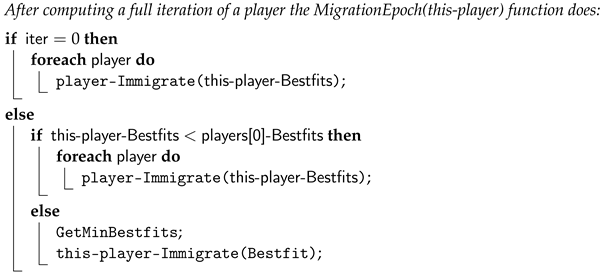
The MigrationEpoch process is responsible for managing the exchange of information between the different players. The definition of this process is what defines most of the hybrid algorithm. For example, it defines the criteria of which individuals migrate between players, how often they migrate, etc. The internal algorithm of the MigrationEpoch process that describes the Hybrid Method presented and tested in this article is detailed in Algorithm 2.

Algorithm 2: Hybrid Method With Gradient Game

The tested Hybrid Method combines two players (i.e., optimization algorithms). One player is intended to perform the exploration of the full search space. The second player is responsible for the exploitation of the promising regions found by the first one. The Hybrid Method shares information between the two players, in a bidirectional way, to overcome the main drawbacks of the optimization algorithms that is formed of. It tries to achieve a fast rate of convergence and to avoid getting stuck at local minimums.

The Hybrid Method initially runs the Genetic Algorithm player. After the first iteration, the best individual found by the Genetic Algorithm is transferred to the conjugate gradient player (first if of the Algorithm 2). The player-Bestfits is the individual with the best objective function found so far, and it is stored for each player. It is updated every time a better individual is found. The conjugate gradient player will use this individual as the starting point of its internal algorithm for its own iteration. The iteration of the conjugate gradient consists of computing the gradient at the location of the starting point and performing a line search in the direction of the gradient. After the iteration of the conjugate gradient, another migration epoch occurs. If the best individual found by the conjugate gradient outperforms the best individual found by the Genetic Algorithm, then the best individual of the conjugate gradient is sent to the Genetic Algorithm.

If the first conditional is not met, a second if condition is evaluated, taking into account the values of the objectives functions achieved so far. The inner if condition compares the objective function of the last evaluated player (this-player) against the objective function of the first player, which in this case is a Genetic Algorithm. The condition this-player-Bestfits < players[0]-Bestfits is clear in a single-objective optimization case, as it is a direct comparison between values of the objective function. If the objective function of this-player is better (lower) than the first player, this individual is migrated to the other player.

If the objective function of this-individual is not better, the inner else part of the algorithm is conducted. In the function GetMinBestfits, a search for the best individual (Bestfit) among all players is performed, and the individual is migrated to this-player, the last player that was executed.

For the full comprehension of the hybrid algorithm, it is important to specify the Immigrate process. This process is defined for each player, and its implementation depends on the type of optimization algorithm, and it affects the general hybrid algorithm. It has one input parameter, the individual that has been selected to migrate into this player. The Immigrate process is responsible for incorporating the individual into the player. The Immigrate process of the Genetic Algorithm substitutes the design variables of the last individual of its internal population with the one that comes from the conjugate gradient. This introduces the genetic information of this individual into the population. In the next iteration, the design variables of this individual will be used in the genetic operators.

In order not to repeat computations, the conjugate gradient player only performs a new iteration when the Genetic Algorithm one provides a best individual different than in the previous global iteration.

On the other hand, the Genetic Algorithm player always incorporates to the population the best individual coming from the conjugate gradient, even if it is the same as in any previous global iteration. The stochastic nature of the Genetic Algorithm can benefit from maintaining the best individual in the population at each iteration. There is a probability that the best individual is not selected in the genetic operators, and to keep the best individual in the population, keeping its genetic information can help to converge in that region. One could think about problems with elitism, but the method only forces one individual to remain in the population, the absolute best so far. If this happens for too long, most probably the optimization has converged, and in case it is not converged, the algorithm should still be capable to explore other regions with the mutation operator and the stochastic nature of the Genetic Algorithm.

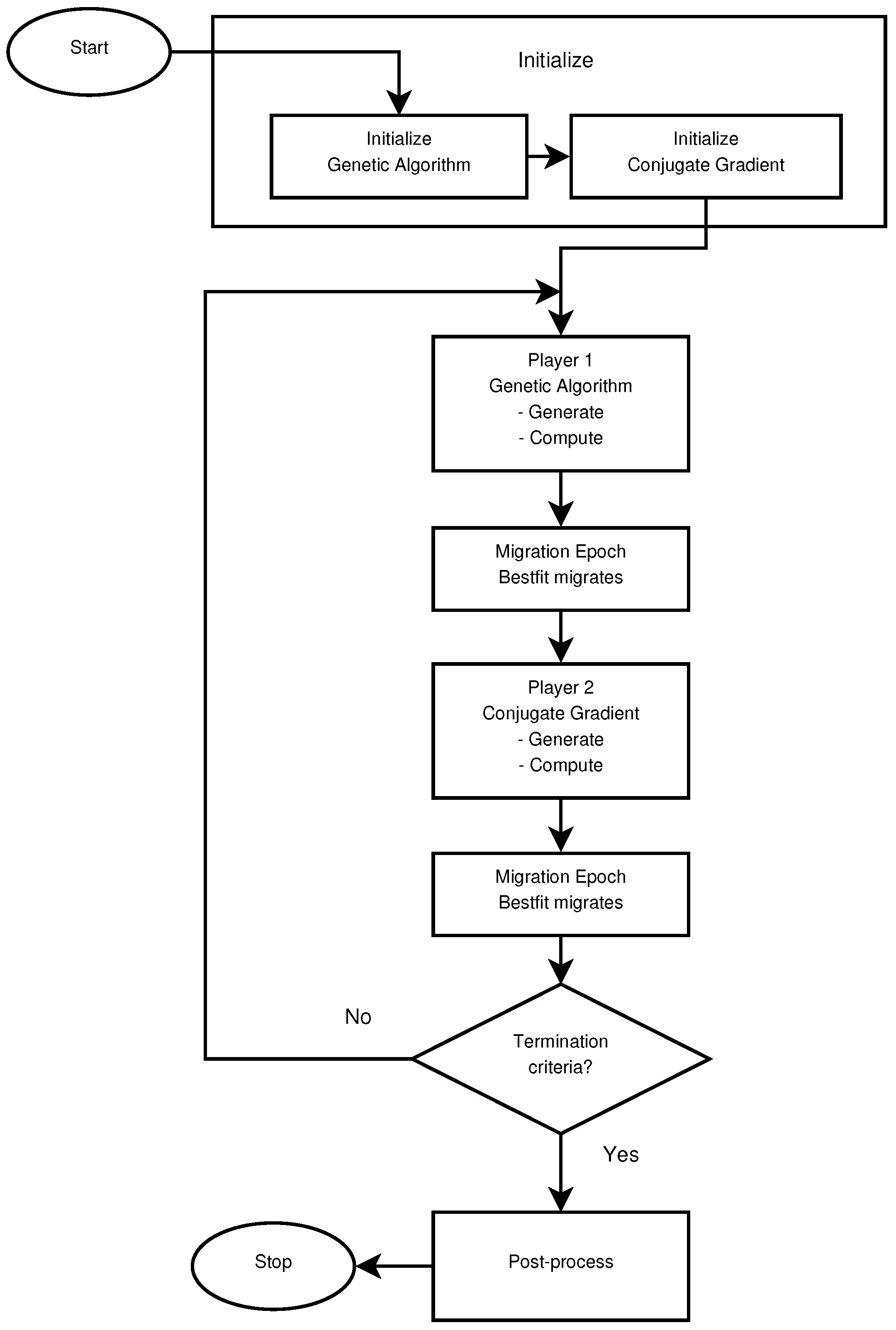
For more clarity, the general algorithm with two players, the Genetic Algorithm as the first player and the conjugate gradient as the second one, is schematized at Figure 1. As mentioned previously, a migration epoch occurs after each iteration of each player. This executes the process detailed in the Algorithm 2, enabling the possibility of exchanging information between the two players.

The configuration of the Genetic Algorithm is specified in

Table 1. Parameters of the Genetic Algorithm.

Parameter	Value
Crossover operator	Simulated Binary Crossover [16]
Mutation operator	Polynomial Mutation [17]
Selection operator	$\mu +\lambda$ & Crowded-Comparison Operator [14]
Probability of crossover	0.9
Probability of mutation	0.1
Population size	20

and the configuration of the conjugate gradient is specified in

Table 2. Parameters of the conjugate gradient algorithm.

Parameter	Value
Search Direction Method	Fletcher-Reeves [18]
Optimal Step Size Method	Golden Section [19]
Epsilon for numerical diferentiation	$1.0\times {10}^{-6}$
First step size	$1.0\times {10}^{-3}$
Optimal step size tolerance	$1.0\times {10}^{-3}$

. The configuration of both optimization algorithms is the same when running alone and when running as a player of the Hybrid Method.

One of the main drawbacks of the proposed Hybrid Method, using both population and gradient-based optimization methods, is that it requires the independent configuration of each optimization method for each player. In this case, the configuration of the Hybrid Method requires the configuration of the Genetic Algorithm and the conjugate gradient players. On the other hand, it also enables the possibility to fine tune the players to perform better, but in cases with high computational costs, it is difficult to perform tests with different configuration values. Another drawback of the Hybrid Method is that the parallelization of the evaluations of the individuals can become more ineffective because each method may have its optimum number of CPUs which may be different for each method. For example, in this case, the evaluation of the Genetic Algorithm population can benefit from using 20 CPUs, one for each individual of the population because they can be computed at the same time. On the other hand, to evaluate the individuals of the conjugate gradient, the parallelization is not that clear. The individuals to compute the gradient can be evaluated at the same time, in this case there are eleven individuals, the central point plus two for each design variable. The line search could also be parallelized, but it is not in the implementation used in this study. The difference in the parallelization capabilities between players could result in an under utilization of the computational resources at some stages of the process.

3. Numerical Results

In order to evaluate the performance of the proposed Hybrid Method, it has been compared against two classical optimization methods, a plain conjugate gradient and a plain Genetic Algorithm. The conjugate gradient method is the same as that which forms part of the Hybrid Method, but running on its own. The Genetic Algorithm used to compare the hybrid algorithm is also the same that forms part of the Hybrid Method, but also running alone. To take into account the random component of the Genetic Algorithm and the strong dependence on the starting point of the conjugate gradient, multiple optimizations with each algorithm have been conducted.

Two optimizations have been conducted with the Genetic Algorithm, starting with different random populations. The Hybrid Method was also run twice, starting with the same random populations as the Genetic Algorithm, so both methods started with the same populations. Finally, the conjugate gradient was run six times, starting with six individuals of the first random population generated by one of the Genetic Algorithms.

All the optimization methods have been tested against the same test case. The test case consists of a single objective optimization of an Active Flow Control optimization problem based on the work of Tousi et al. [20]. The objective of that work is to determine the optimum parameters of the Synthetic Jet actuator design at different angles of attack in a multiple objective optimization problem. The test case details for the comparison of optimization algorithms are presented in Section 3.1.

3.1. Test Case Description

The test case focuses on the optimization of an Active Flow Control device, more precisely, a Synthetic Jet actuator. The device is tested on a SD7003 airfoil at an angle of attack of 14 degrees. For the comparison between the optimization algorithms, which is the main objective of this work, a single optimization problem with five design variables has been used. The objective function is to maximize the lift coefficient, and to do so the objective function is set to:

$$f=-C_l$$

At high angles of attack, the Synthetic Jet can greatly affect the flow structure, improving the lift coefficient. The Synthetic Jet actuator, if set properly, can help to reattach the flow to the airfoil or to almost avoid the detachment of the flow.

The design variables are the same as the previous work by Tousi et al. [20]. For a full explanation and detail of the Synthetic Jet actuator design variables meaning refer to [20]. The five design variables are:

$F^{+}$

Non-dimensional frequency.

$C_{\mu }$

Momentum coefficient.

$\theta$

Jet inclination angle.

$x/C$

Non-dimensional jet position.

$h/C$

Non-dimensional jet width.

The evaluation range of each design variable is shown in

Table 3. Active Flow Control design variables and their evaluation ranges.

Design Variable	Minimum Value	Maximum Value
$F^{+}$	0.1	10
$C_{\mu }$	0.0001	0.02
${\theta }^o$	5	175
$x/C$	0.001	0.3
$h/C$	0.005	0.015

. The same ranges are used with all optimization algorithms.

The flow has been solved with an unsteady Reynolds averaged Navier–Stokes model (URANS), using the OpenFOAM software. Other models, like direct numerical simulation (DNS) or large eddy simulation (LES) could be used to solve the Synthetic Jet simulation, but their computational cost is too high to perform so many optimizations with the available resources. In addition, there is no need to use such precise solvers to evaluate the performance of the Hybrid Method. More details on the solver used can be consulted at [20], as this study uses the same model.

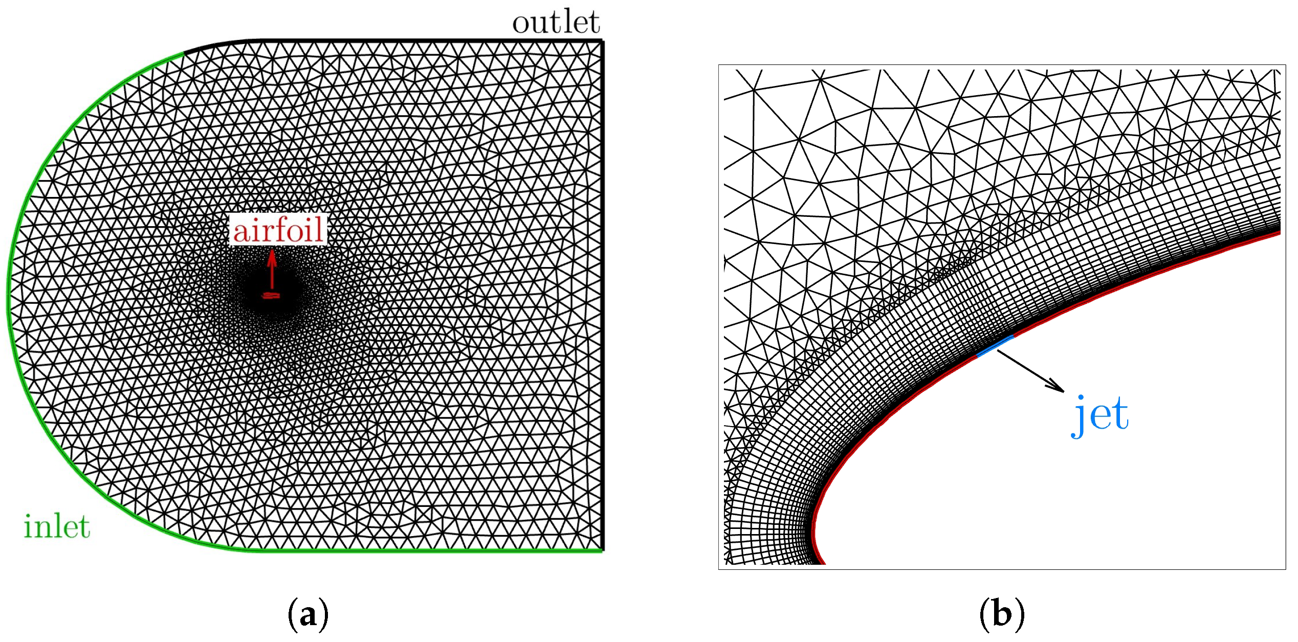
The mesh used, see Figure 2a, is one of the meshes previously evaluated in [20], although having a smaller number of cells (34,448) than the final one employed in that paper, the maximum $y^{+}$ after the simulation was $y^{+}=1$. The mesh nearby the Synthetic Jet actuator is presented in Figure 2b. The run time of the simulation has been adjusted to 30 time units, which as shown in [20] is sufficient to reach convergence. It is important to note that this study is not about the Synthetic Jet actuator optimization, but to compare the optimization algorithms in a real world application with a significant computational cost and complexity. The study of the physical problem is not the main purpose of this study, which justifies reducing the precision of each CFD simulation in order to reduce the overall computational cost.

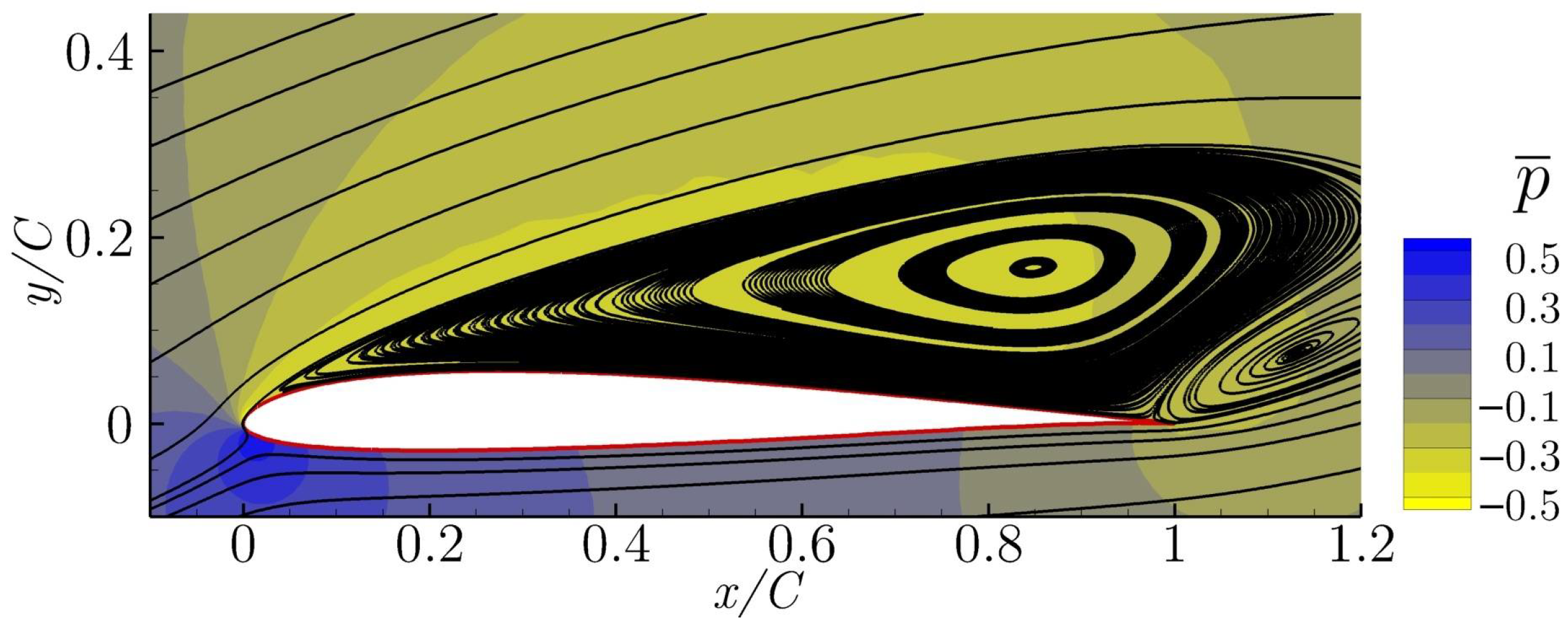
In Figure 3, the temporal averaged streamlines and pressure field for the non-actuated case is presented. This configuration is called the baseline. From the streamlines, it can be seen that the flow is fully separated and the airfoil is under stall conditions.

3.2. Results from the Optimizations Methods

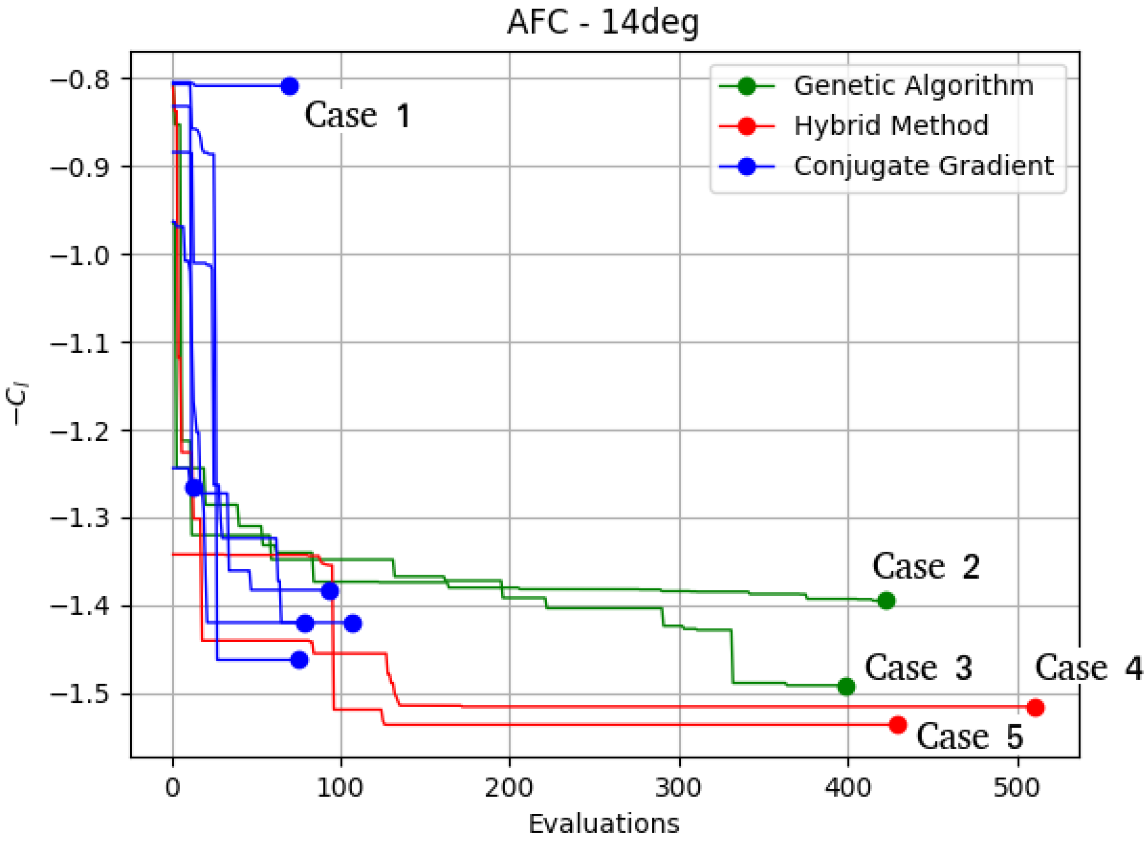
This section introduces the results obtained for the proposed comparison. The convergence of the different optimization algorithms are shown in Figure 4. The results shown in the graph of Figure 4 reflect the problems encountered by the gradient based method. Most runs of the conjugate gradient initially improve faster than the Genetic Algorithm but then get stuck between $C_l\approx 1.35$ and $C_l\approx 1.45$ (except for two runs that get stuck at $C_l\approx 0.8$ and $C_l\approx 1.25$, respectively). Those lift coefficient values are achieved with almost 100 evaluations of the objective function for each optimization of the conjugate gradient. The strong dependence of the conjugate gradient on the starting point is also reflected on these results, as it presents very different solutions between runs than the other methods. In all cases, the conjugate gradient method was stopped because the algorithm found a local minimum and could not compute the gradient to further improve the results.

On the other hand, the Genetic Algorithm provides optimal solutions similar to the conjugate gradient, but with a higher computational cost, approximately four times higher. Both runs of the Genetic Algorithm achieve values of the objective function in the range of the conjugate gradient results. One of the runs achieves a better objective function than all of the conjugate gradient runs, with a value of $C_l=1.49$. It is important to note that the Genetic Algorithm optimizations could run additional iterations and achieve better results, but with a high computational cost.

The Hybrid Method is the method that achieved better results, outperforming all runs of the other algorithms in both of its runs. During the first iterations, it achieved a convergence rate similar to the conjugate gradient. However, the improvement of the solution has continued, avoiding being trapped in any local minimum. It is also the most robust, as both runs are very similar in their performance. Both Hybrid Method runs outperformed all the other optimization methods with a $C_l=1.52$ and $C_l=1.54$. One run of the Genetic Algorithm achieved a comparable solution ($C_l=1.49$), but it took more than twice the computational cost of the Hybrid Method. Case 3, with a lift coefficient of $C_l=1.49$, obtained by the Genetic Algorithm with around 375 objective function evaluations, improves the baseline lift coefficient by $86\%$. Cases 4 and 5, obtained by the Hybrid Method runs, achieved a lift coefficient of $C_l=1.52$ and $C_l=1.54$, respectively. Both runs needed around 125 objective function evaluations, which is $67\%$ the number of evaluations of case 3, with an increase in the lift coefficient of $90\%$ and $93\%$, respectively, from the baseline. The best lift coefficient achieved by each optimization is presented in

Table 4. Best lift coefficient of each optimization case, means and standard deviation.

	Genetic Algorithm	Hybrid Method	Conjugate Gradient
$C_l$	1.39	1.52	0.81
			1.26
			1.38
	1.49	1.54	1.42
			1.42
			1.46
$\overline{C_l}$	1.44	1.53	1.29
$\sigma$	0.07071	0.01414	0.2458

. The mean ($\overline{C_l}$) and standard deviation ($\sigma$) of the lift coefficient achieved by each optimization method is also presented. The Hybrid Method presents the best lift coefficient mean ($C_l=1.53$) followed by the Genetic Algorithm ($C_l=1.44$) and the conjugate gradient ($C_l=1.29$). The conjugate gradient is the least robust, with a standard deviation of $\sigma =0.2458$, but four of the six optimizations achieved similar results than the Genetic Algorithm with less computational effort.

Looking at these results, one can conclude that the proposed Hybrid Method performs much more robustly than the conjugate gradient method and much faster than the Genetic Algorithm.

3.3. Results Based on the Fluid Flow Performance

This subsection provides a comparison between the characteristics of the flow field corresponding to each of the optimal solutions labeled in Figure 4. The lift coefficient and design variables of each of the optimal solutions are presented in

Table 5. Values of the lift coefficient and design variables of the five labeled cases.

Case	${\mathit{C}}_{\mathit{l}}$	${\mathit{F}}^{+}$	${\mathit{C}}_{\mathit{\mu }}$	${\mathit{\theta }}^{\mathit{o}}$	$\mathit{x}/\mathit{C}$	$\mathit{h}/\mathit{C}$
1	0.81	8.6	$1\times {10}^{-4}$	136	$3\times {10}^{-1}$	$5\times {10}^{-3}$
2	1.39	0.3	$1.47\times {10}^{-2}$	24	$1\times {10}^{-3}$	$1.4\times {10}^{-2}$
3	1.49	3.2	$1.92\times {10}^{-2}$	8	$2\times {10}^{-2}$	$5\times {10}^{-3}$
4	1.52	6.7	$2\times {10}^{-2}$	7	$2.6\times {10}^{-2}$	$5\times {10}^{-3}$
5	1.54	9.9	$2\times {10}^{-2}$	5	$1.97\times {10}^{-2}$	$5\times {10}^{-3}$

. For a full explanation of the flow structure and details on the Synthetic Jet actuator performance, the reader is directed to [20].

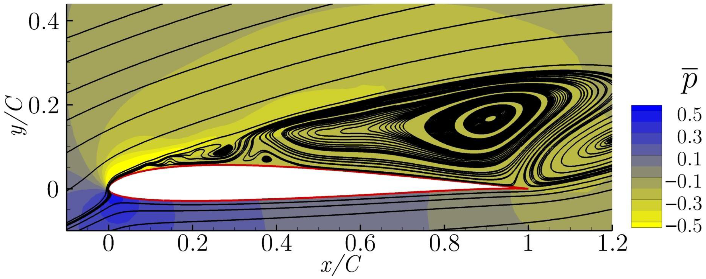
As explained in the Section 3.1, the flow without the Synthetic Jet actuator is fully detached, see Figure 3. The objective of the Synthetic Jet actuator is to prevent or minimize flow separation. The averaged streamlines and pressure field of the optimized cases are presented and discussed in this section. The flow field corresponding to Case 1 is presented in Figure 5. Despite the fact that the flow separation is slightly delayed versus the baseline case, a large vortical structure is still observed over the airfoil.

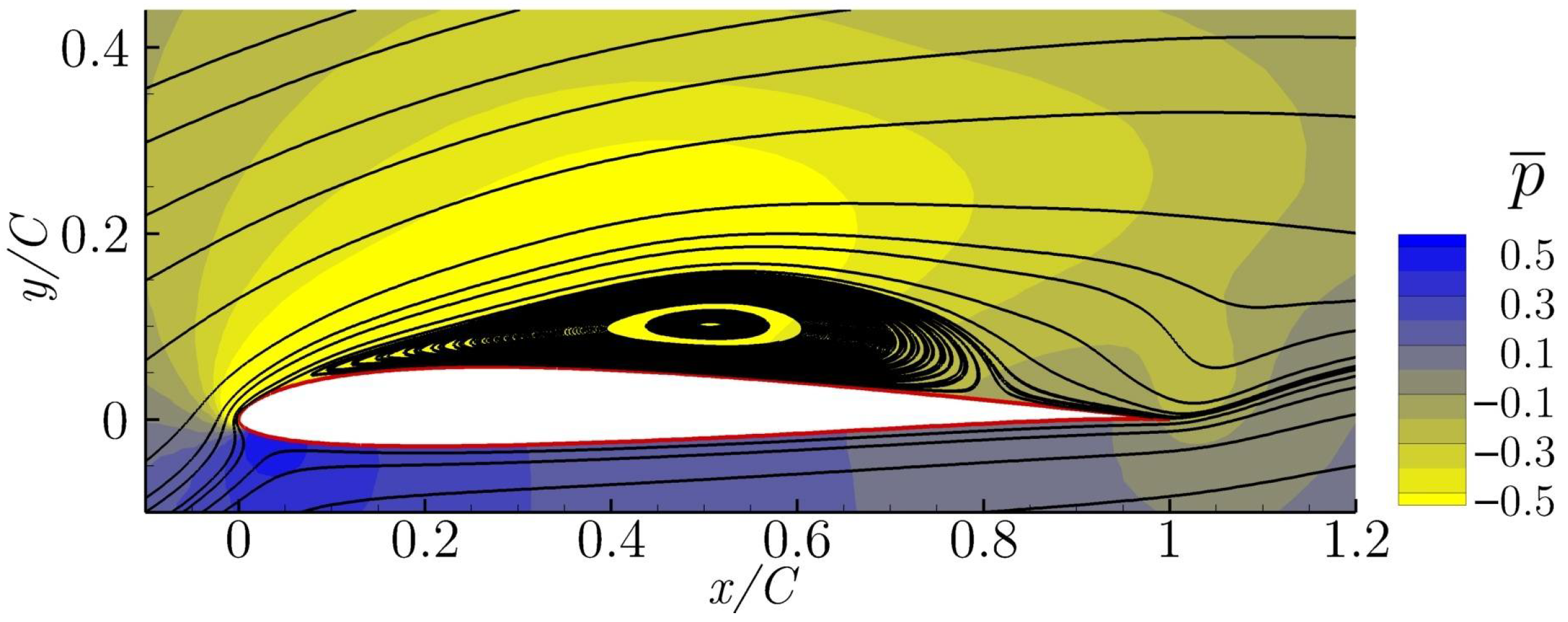
In Figure 6, the averaged streamlines and pressure field obtained from case 2 is presented. It shows a late reattachment of the flow, which improves the lift coefficient of the baseline by $74\%$. This solution has been obtained by one of the Genetic Algorithm’s runs, with around 400 evaluations of the objective function. The resulting lift coefficient is $C_l=1.39$.

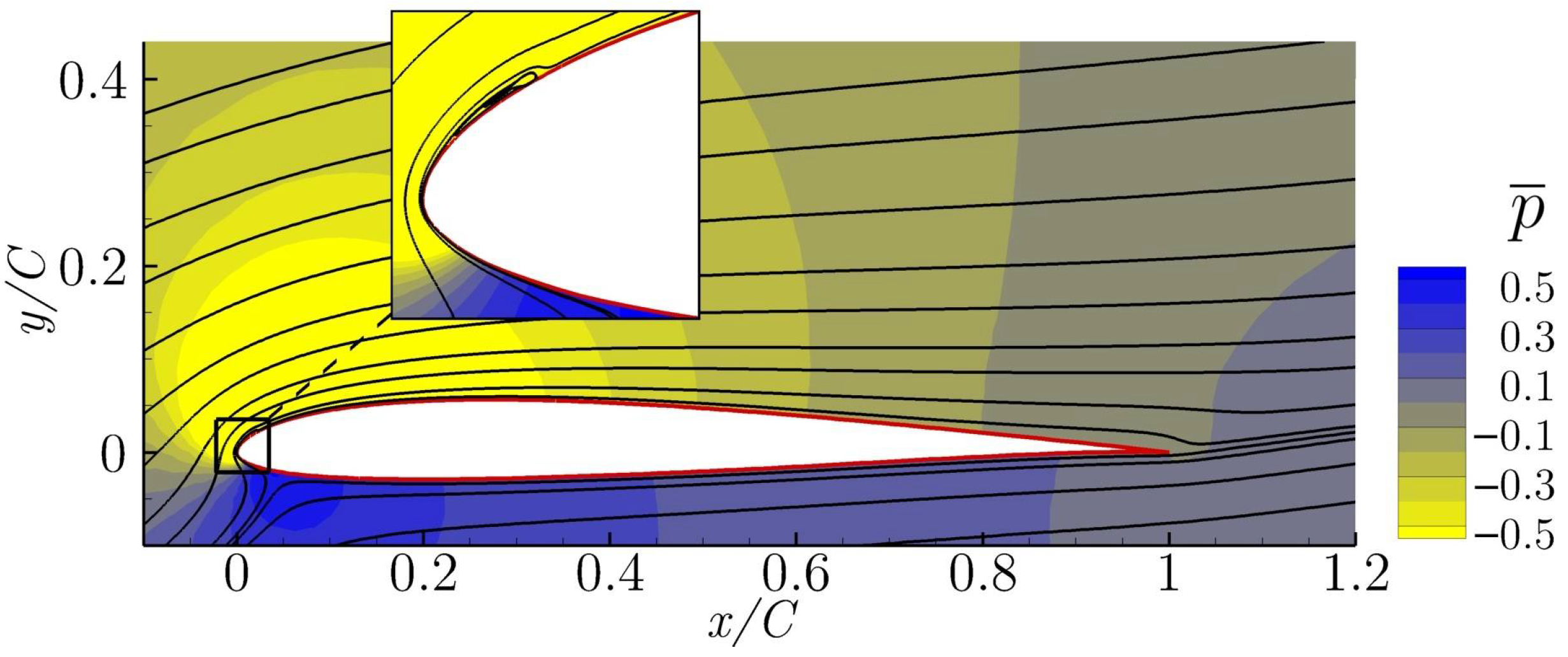
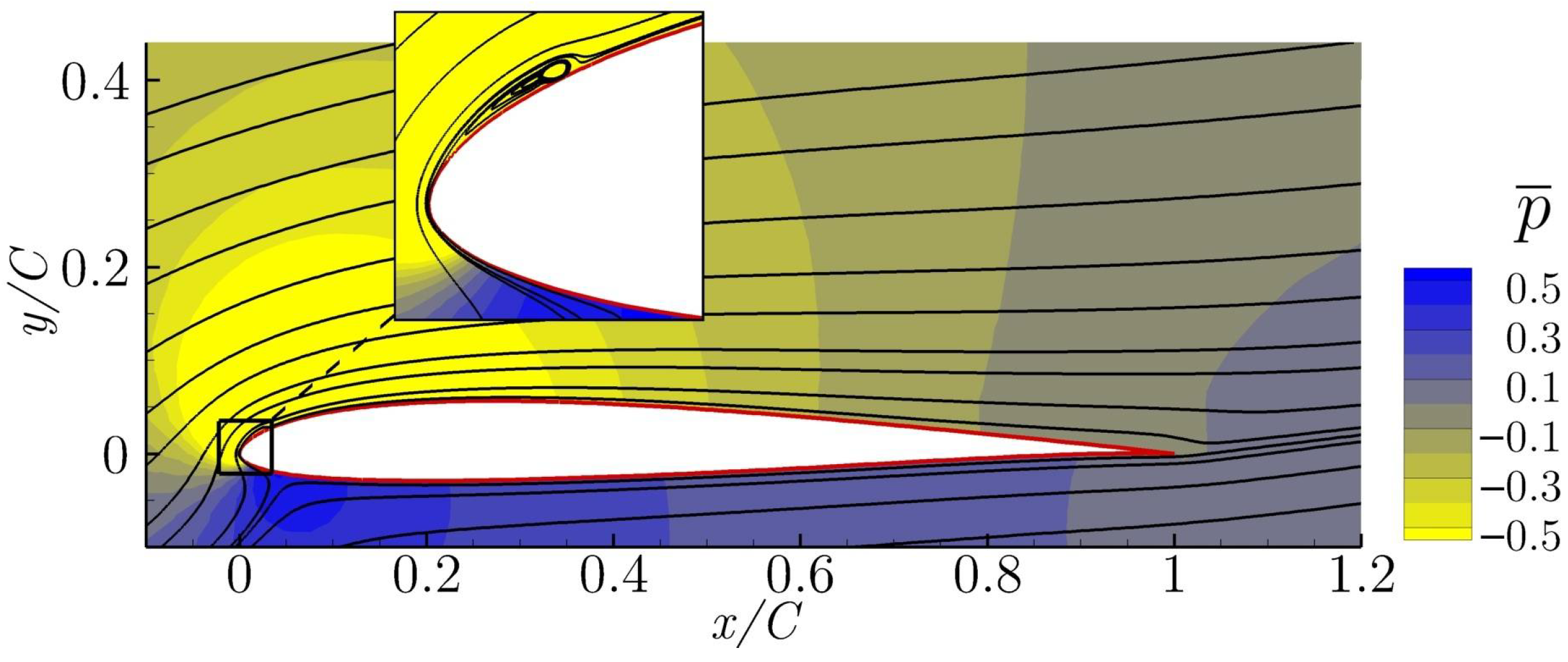
The averaged streamlines and pressure fields of cases 3, 4 and 5 are presented in Figure 7, Figure 8 and Figure 9, respectively. All of them show a complete flow reattachment, with very minor differences in the size of the laminar bubble appearing close to the airfoil leading edge. The bubbles are in fact located near the Synthetic Jet position, just downstream of it, as can be seen in the above mentioned figures. The optimization of the flow control actuation parameters has managed to successfully reattached the flow along the entire airfoil chord.

4. Discussion

This article presents a new Hybrid Method which combines two optimization methods (a Genetic Algorithm and a conjugate gradient) of a very different nature. The test case used to evaluate the performance of the new Hybrid Method is a single objective optimization with five design variables associated with a Synthetic Jet actuator. The CFD simulations are solved using a URANS model, which has proven precise enough to capture the active flow actuator effect and to compare between different designs. For the test case of the Synthetic Jet actuator, the Hybrid Method has outperformed both of the traditional optimization algorithms. The new Hybrid Method successfully combines the best characteristics of both optimization algorithms. It shows a great convergence rate, like a gradient based method, but without the lack of robustness that usually comes with gradient based methods and complex applications. The increase in robustness is provided by the Genetic Algorithm player which avoids local minimums. The strategy to exchange information between the two optimization algorithms proposed in this Hybrid Method has proven efficient to overcome the main drawbacks of both classical optimization methods, and the result is an optimization method capable of exploring and exploiting the full search space.

The future work aims to further test the new Hybrid Method in a multi-objective optimization problem such as the one introduced in Tousi et al. [20]. In high CPU demanding applications, such a Synthetic Jet actuator optimization is important when working with optimization algorithms that require a low number of evaluations of the physical model, and the new Hybrid Method has proven a good option.