Aerodynamic Efficiency Improvement on a NACA-8412 Airfoil via Active Flow Control Implementation

Abstract

The present paper introduces a parametric optimization of several Active Flow Control (AFC) parameters applied to a NACA-8412 airfoil at a single post-stall Angle of Attack (AoA) of ${15}^{\circ }$ and Reynolds number $Re$ = $68.5\times {10}^3$. The aim is to enhance the airfoil efficiency and to maximize its lift. The boundary layer separation point was modified using Synthetic Jet Actuators (SJA), and the airfoil optimization was carried on by systematically changing the pulsating frequency, momentum coefficient and jet inclination angle. Each case has been evaluated using Computational Fluid Dynamic (CFD) simulations, being the Reynolds Averaged Navier–Stokes equations (RANS) turbulence model employed the Spalart Allmaras (SA) one. The results clarify which are the optimum AFC parameters to maximize the airfoil efficiency. It also clarifies which improvement in efficiency is to be expected under the operating working conditions. An energy balance is presented at the end of the paper, showing that for the optimum conditions studied the energy saved is higher than the one needed for the actuation. The paper clarifies how a parametric analysis has to be performed and which AFC parameters can be initially set as constant providing sufficient previous knowledge of the flow field is already known. A maximum efficiency increase versus the baseline case of around 275% is obtained from the present simulations.

1. Introduction

The Active Flow Control (AFC) technology applied to airfoils is beginning to be of common use, then a considerable number of recent papers tackle this matter [1,2,3]. Parametric analysis is still the most common methodology employed to evaluate the effect of the AFC on airfoils, yet the use of optimizers is becoming popular to obtain the most appropriate AFC parameters in any given application [4,5]. Some initial studies analyzed the performance when using continuous and pulsating actuations, and it was soon discovered that pulsating flow was coupling with the boundary layer natural instabilities and so being more energetically efficient [6,7,8].

Airfoil aerodynamic efficiency decisively effect fuel consumption, and AFC can improve it. Briefly, the AFC technology adds or subtracts momentum to/from the main flow with the aim of interacting with the boundary layer and delaying or advancing its separation. One of the advantages over passive flow control is that it is not creating drag increase when operating outside the design conditions. Cattafesta and Sheplak [9] divided the AFC techniques into three categories. (1) Moving body actuators, they do not add or substract mass and induce local fluid motion [10]. (2) Plasma actuators, they generate high frequency ionized jets of fluid [11,12,13,14]. (3) Fluidic actuators (FA), create pulsating flow and in some configurations no moving parts are required. In some particular FA designs, the origin of the self-sustained oscillations was recently unveiled in [15,16,17].

From the different sorts of FA, Zero Net Mass Flow Actuators (ZNMFA) also called Synthetic Jet Actuators (SJA), have gained particular attention in the scientific community due to their high capabilities in controlling boundary layer separation [18,19,20,21]. Another advantage of SJAs is that do not require external fluid supply.

When considering the implementation of SJAs, two parameters are particularly relevant: the non-dimensional frequency $F^{+}=fC/U_{\infty }$, where f is the dimensional frequency, C the airfoil chord and $U_{\infty }$ the free-stream velocity, and the momentum coefficient ($C_{\mu }$). $C_{\mu }$ is defined as $C_{\mu }=(h{\rho }_{jet}\left(U_j^2\right)sin\theta )/\left(C{\rho }_{\infty }\left(U_{\infty }^2\right)\right)$, where h is the jet width, ${\rho }_{jet}$ is the jet density and ${\rho }_{\infty }$ is the far field one, $U_j$ characterizes the jet maximum velocity, the parameter $\theta$ defines the inclination angle of the jet versus the adjacent surface.

Amitay et al. [22] and Amitay and Glezer [23] studied the SJA frequency, position and $C_{\mu }$ when applied to a symmetric airfoil and observed that when locating the actuator near to the boundary layer separation point, the momentum coefficient needed to reattach the flow was smaller. Regarding the actuation frequency, they found that when it was an order of magnitude higher than the vortex shedding one ($F^{+}\mathcal{O}\left(10\right)$), the flow was completely reattached.

SJAs on a NACA-0015 airfoil at $Re$ = $8.96\times {10}^5$ were experimentally studied by Gilarranz et al. [24]. They increased the stall angle from ${12}^{\circ }$ to ${18}^{\circ }$ and observed that for AoA $>{10}^{\circ }$, the effectiveness of the actuation considerably increased. At AoA $>{25}^{\circ }$, considerably high actuation frequencies were needed to observe large flow variations. The same airfoil and Reynolds number was studied by You and Moin [25] using Large Eddy Simulation (LES). A lift increase of 70% was obtained when using $C_{\mu }$ = 0.0123, $F^{+}$ = 1.284 and $\theta$ = 30.2°. The same airfoil at $Re$ = $3.9\times {10}^4$ was experimentally studied by Tuck and Soria [26]. The optimum momentum coefficient and actuation frequencies were respectively, $C_{\mu }$ = 0.0123O and $F^{+}$ = 0.7 and $1.3$, being the highest frequency the most effective one. When using these forcing conditions, an improvement of the stall AoA from ${10}^{\circ }$ to ${18}^{\circ }$ was observed. Kitsios et al. [27] numerically studied the same airfoil and Reynolds number via LES simulations. They observed that the optimal frequencies coincided with the vortex shedding one obtained from the baseline case ($f_{wake}$) and its first harmonic ($2f_{wake}$). Buchmann et al. [28] reached the same conclusion through experimental tests. Flow control using SJAs on a NACA-23012 at $Re$ = $2.19\times {10}^6$ was numerically investigated by Kim and Kim [29], Monir et al. [30]. Maximum lift was obtained when the jet was placed nearby the boundary layer separation point and $F^{+}$ = 1. When applying SJA tangentially, clear advantages were observed than when injecting/sucking fluid perpendicular to the surface.

The separation control generated by SJA on a NACA-0025 airfoil at $Re$ = ${10}^5$ and AoA = $5^{\circ }$ were experimentally studied by Goodfellow et al. [31]. Momentum coefficient was found to be the primary control parameter, a drag decrease of nearly $50\%$ was obtained when $C_{\mu }$ was higher than a certain threshold value. The same Reynolds number and wing profile, but at AoA = ${10}^{\circ }$ was evaluated by Feero et al. [32]. They observed that the momentum coefficient needed $C_{\mu }$ to keep the flow reattached, was an order of magnitude lower when the excitation frequencies happened to be around the vortex shedding one. The same Reynolds number and wing profile but at AoA = ${12}^{\circ }$ was analyzed in [33], where the jet position effectiveness in controlling the flow separation was evaluated. The optimum results were obtained when locating the jet groove nearby (whether downstream or upstream) the boundary layer separation point, a small improvement was observed in the upstream location. The NACA-0018 profile at AoA = ${10}^{\circ }$ and at $Re$ = 1000, was evaluated using direct numerical simulation (3D-DNS) by Zhang and Samtaney [34]. Three non-dimensional frequencies ($F^{+}$ = 0.5, 1 and 4) were considered. The optimum frequency was $F^{+}$ = 1 although improvement was observed in all of them. In Rodriguez et al. [35], the SD7003 airfoil at $Re$ = $6\times {10}^4$ and under three AoA = $4^{\circ }$, ${11}^{\circ }$ and ${14}^{\circ }$ was numerically studied. At AoA = ${14}^{\circ }$ they obtained an aerodynamic efficiency increase of 124%. The same Reynolds number and wing profile but at AoA = ${14}^{\circ }$, and AoA = ${13}^{\circ }$ & ${16}^{\circ }$ was studied by [4,5], respectively. Due to the fact that in these studies optimization processes were employed, the maximum efficiency increase was obtained to be 280% and 591%, respectively.

The airfoil chosen for the present study is the NACA-8412, a Reynolds number of $Re$ = $68.5\times$${10}^3$ and AoA = ${15}^{\circ }$ were considered. According to the authors knowledge no previous studies for this airfoil and Re configuration have been found in the literature. The usage of the NACA-8412 airfoil was motivated by its large curvature, which in combination with the high AoA used will produce a separation of the flow close to the leading edge. This early separation will remark the effects of introducing SJA, and enable a clearer comparison of the results with the baseline case. Furthermore, the methodology employed in the present manuscript, which is based on a previous knowledge of the flow field and consist in initially fixing some AFC parameters, is proven to be very useful in obtaining good results while saving computational resources.

The rest of the manuscript is structured as follows. The formulation of the problem, the numerical methods employed and the mesh independence study are presented in Section 2. The definition of the AFC parameters and their implementation are introduced in Section 3. The Results section is introduced in Section 4 and the summary of the work is presented in Section 5.

2. Numerical Method

2.1. Governing Equations and Turbulence Model

Due to the unsteadiness of the problem, three possible turbulence models arose: Direct Numerical Simulation (DNS), Large Eddy Simulations (LES) and Unsteady Reynolds Averaged Navier–Stokes (URANS). Due to the large computational power required to perform both DNS and LES simulations, URANS was selected as the turbulence model used. More specifically, the Spalart–Allmaras model was chosen to perform all the simulations involved in the present study because of its suitability for low Reynolds cases and its easy convergence when the Courant–Friedrichs–Levy number $CFL<1$. The Navier–Stokes equations for incompressible flow, take the form:

$$\frac{\partial u_i}{\partial x_i}=0$$

(1)

$$\frac{\partial u_i}{\partial t}+\frac{\partial u_i{u}_j}{\partial x_j}=-\frac{1}{\rho }\frac{\partial p}{\partial x_i}+\nu \frac{{\partial }^2{u}_i}{\partial x_j\partial x_j}$$

(2)

Substituting each variable $\varphi$ by the average $\overline{\varphi }$ and fluctuation ${\varphi }^{\prime }$ terms.

$$\varphi =\overline{\varphi }+{\varphi }^{\prime }$$

(3)

Being $\varphi (x,t)$ a generic flow variable, it can be written as the sum of its mean $\overline{\varphi }(x,t)$ and fluctuating components ${\varphi }^{\prime }(x,t)$, being $\varphi (x,t)=\overline{\varphi }(x,t)+{\varphi }^{\prime }(x,t)$. By substituting it in the Navier–Stokes equations and taking the time average, it results in the following Reynolds-averaged Navier–Stokes equations,

$$\frac{\partial {\overline{u}}_i}{\partial x_i}=0$$

(4)

$$\frac{\partial {\overline{u}}_i}{\partial t}+\frac{\partial {\overline{u}}_i{\overline{u}}_j}{\partial x_j}=-\frac{1}{\rho }\frac{\partial \overline{p}}{\partial x_i}+\nu \frac{{\partial }^2{\overline{u}}_i}{\partial x_j\partial x_j}-\frac{\partial \overline{u_i^{\prime }{u}_j^{\prime }}}{\partial x_j}$$

(5)

where the term $\overline{u_i^{\prime }{u}_j^{\prime }}$ is the Reynolds stress tensor denoted by $R_{ij}$ and was approximated using Boussinesq hypothesis. The deviatoric part of the tensor is given as follows,

$$R_{ij}-\frac{1}{3}{R}_{kk}{\delta }_{ij}=-2{\nu }_t{\overline{S}}_{ij}$$

(6)

where ${\nu }_t$ is the kinematic eddy viscosity that needs to be modeled using one of the RANS models.

As it has been previously mentioned, the turbulence model selected was the Spalart–Allmaras (S-A). The model proposed by [36] solves a single transport equation for the modified form of the turbulent kinetic energy called $\tilde{\nu }$. This new parameter is identical to ${\nu }_t$ except in the viscous-affected region nearby the wall.

$${\nu }_t=\tilde{\nu }\left(\frac{{\chi }^3}{{\chi }^3+C_{v1}^3}\right)$$

(7)

The transport equation of $\tilde{\nu }$ is given as:

$$\begin{array}{c}\hfill \frac{\partial \tilde{\nu }}{\partial t}+u_j\frac{\partial \tilde{\nu }}{\partial x_j}=\frac{1}{\sigma }\left[\frac{\partial }{\partial x_j}\left((\nu +\tilde{\nu })\frac{\partial \tilde{\nu }}{\partial x_j}\right)+C_{b2}\frac{\partial \tilde{\nu }}{\partial x_i}\frac{\partial \tilde{\nu }}{\partial x_i}\right]+C_{b1}(1-f_{t2})\tilde{S}\tilde{\nu }-\left[C_{w1}{f}_w-\frac{C_{b1}}{{\kappa }^2}{f}_{t2}\right]{\left(\frac{\tilde{\nu }}{d}\right)}^2\end{array}$$

(8)

where:

$$\begin{array}{c}{f}_{\omega }=g{\left[\frac{1+C_{\omega 3}^6}{g^6+C_{\omega 3}^6}\right]}^{1/6},g=r+C_{\omega 2}(r^6-r),r=min\left[\frac{\tilde{\nu }}{\tilde{S}{\kappa }^2{d}^2},10\right]\hfill \\ \tilde{S}=\mathsf{\Omega }+\frac{\tilde{\nu }}{{\kappa }^2{d}^2}{f}_{v2},f_{t2}=C_{t3}exp(-C_{t4}{\chi }^2),f_{v2}=1-\frac{\chi }{1+\chi f_{v1}}\hfill \\ f_{v1}=\frac{{\chi }^3}{{\chi }^3+C_{v1}^3},\chi =\frac{\tilde{\nu }}{\nu }\hfill \end{array}$$

(9)

Being d the distance from a given point to the nearest wall, and $\mathsf{\Omega }$ the magnitude of the vorticity. The model constants have the following default values:

$$\begin{array}{c}{C}_{b1}=0.1355,C_{b2}=0.622,\sigma =\frac{2}{3},C_{\omega 1}=\frac{C_{b1}}{{\kappa }^2}+\frac{\left(1+C_{b2}\right)}{\sigma }\hfill \\ C_{\omega 2}=0.3,C_{\omega 3}=2.0,C_{v1}=7.1,\kappa =0.4187,C_{t3}=1.2\hfill \\ C_{t4}=0.5\hfill \end{array}$$

(10)

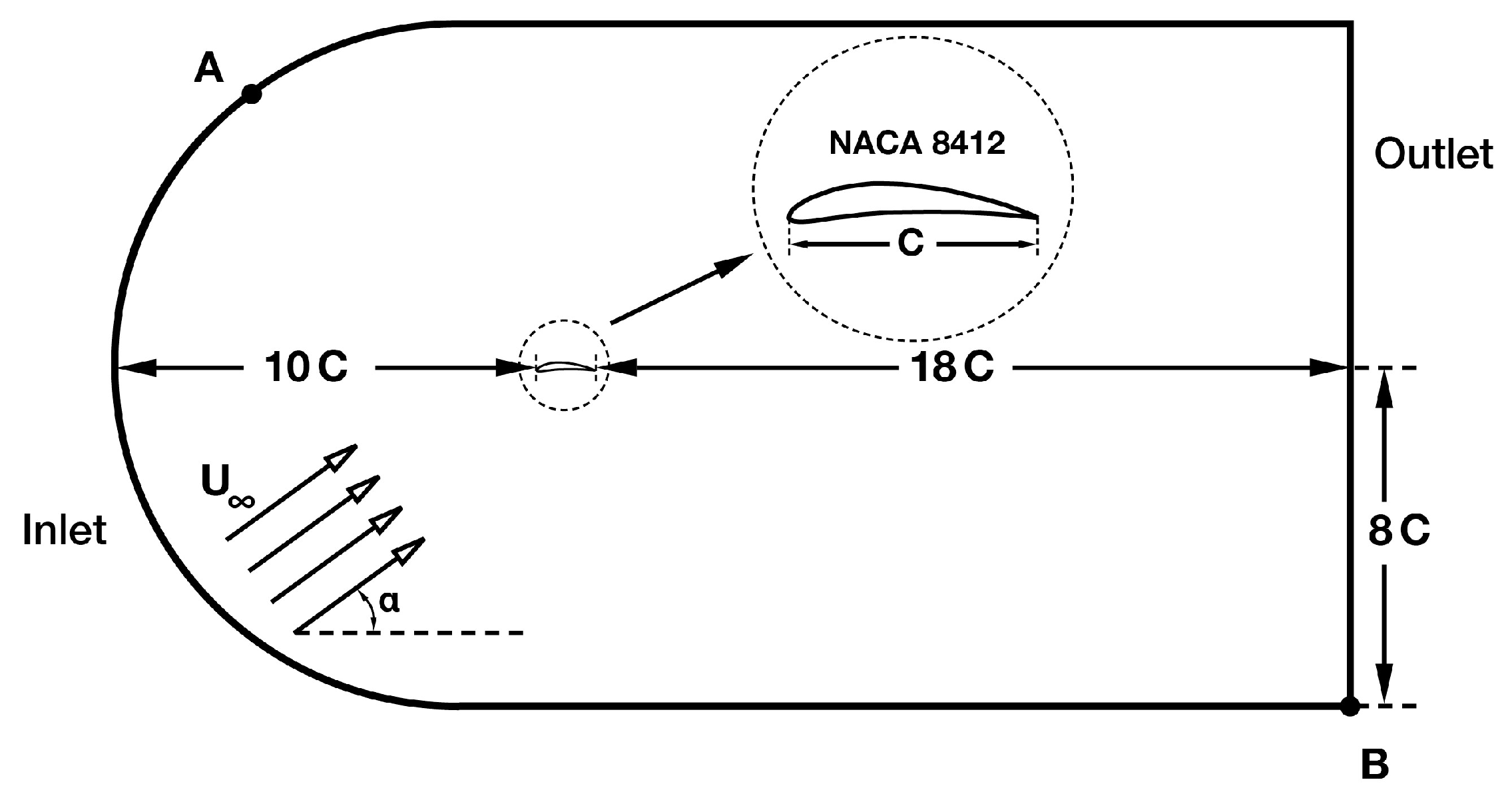
2.2. Numerical Domain and Boundary Conditions

The NACA-8412 airfoil’s leading edge (LE) was located at the origin of the coordinate system, and the airfoil was fixed at zero degree angle with respect to the x-axis. The post-stall angle of attack of ${15}^{\circ }$ was introduced by decomposing the freestream velocity in the corresponding x and y components. Note that all distances have been expressed as function of the airfoil chord C (see Figure 1). The distance between the inlet and the LE following the x-axis was set at 10C, while the distance between the trailing edge (TE) and the outlet was set at 18C. The height of the domain is 16C, symmetrically distributed with respect to the airfoil. An almost identical computational domain was recently employed in [4].

The inlet was defined by the line connecting points A and B (see Figure 1) in a counter-clockwise direction, while the outlet was defined by the line connecting A and B in clockwise direction. At the inlet, Dirichlet boundary conditions for velocity were set by imposing the decomposition of the freestream velocity as it has been previously mentioned. Regarding pressure, Neumann boundary conditions were used. At the outlet, Neumann boundary conditions for velocity and Dirichlet boundary conditions for pressure were imposed. Over the airfoil’s surface Dirichlet boundary conditions for velocity were imposed in order to guarantee the non-slip condition, Neumann boundary conditions for pressure were considered.

The point A represented in Figure 1, which corresponds to one of the connecting points between the inlet and the outlet, had to guarantee that the angle formed by its tangent was larger than the angle of attack studied (AoA = ${15}^{\circ }$). For the present configuration, the tangent line to the inlet curve at the point A and the horizontal form an angle of 36.87°, complying with the mentioned restriction. Figure 2 introduces some AFC parameters as the jet position, jet width and jet inclination angle. The International Standard Atmosphere (ISA) model at sea level was used to select the air density, the pulsating flow fluid density, as well as the fluid dynamic viscosity. A relatively low Reynolds number was selected in order to have proportionally low mesh computational requirements and computational time. The values of the physical parameters involved in the present study are summarized in

Table 1. Physical conditions.

Reynolds number $\left(\mathit{R}\mathit{e}\right)$	68.5 × ${10}^3$
Freestream velocity ($U_{\infty }$)	1 m/s
Kinematic Viscosity ($\nu$)	1.4599 × ${10}^{-5}$ m2/s
Density ($\rho$)	1.225 kg/m3
Pulsating flow fluid density (${\rho }_j$)	1.225 kg/m3
Angle of attack ($\alpha$)	15°
Chord length (C)	1 m

.

2.3. Non-Dimensional Parameters

In this section the non dimensional groups used along the paper are introduced.

Reynolds number

$$Re=\frac{U_{\infty }C}{\nu }$$

(11)

where $U_{\infty }$ is the free-stream velocity, C the chord length and $\nu$ the fluid kinematic viscosity.

Lift coefficient

$$C_l=\frac{2F_l}{\rho C{U}_{\infty }^2}$$

(12)

where $\rho$ is the free-stream fluid density, and $F_l$ the dimensional lift force.

Drag coefficient

$$C_d=\frac{2F_d}{\rho C{U}_{\infty }^2}$$

(13)

where $F_d$ is the dimensional drag force. Note that the lift and drag coefficients are a function of the angle of attack (AoA) and Reynolds number.

Aerodynamic efficiency

$$E=\frac{F_l}{F_d}=\frac{C_l}{C_d}$$

(14)

Pressure coefficient

$$C_P=\frac{P-P_{\infty }}{\frac{1}{2}\rho U_{\infty }^2}$$

(15)

The parameter P is the generic static pressure and $P_{\infty }$ is the free-stream one.

Friction coefficient

$$C_F=\frac{{\tau }_w}{\frac{1}{2}\rho U_{\infty }^2}$$

(16)

where ${\tau }_w$ are the wall shear stresses.

Dimensionless wall distance

$$y^{+}=\frac{u_{\tau }y}{\nu }$$

(17)

With:

$$u_{\tau }=\sqrt{\frac{{\tau }_w}{\rho }}$$

(18)

$u_{\tau }$ characterizes the friction velocity and y is the dimensional distance with respect to the wall.

Jet momentum coefficient

$$C_{\mu }=\frac{h\left(\rho U_{max}^2\right)\sin {\theta }_j}{C\left(\rho U_{\infty }^2\right)}$$

(19)

where h characterizes the jet width, $U_{max}$ is the maximum jet velocity and ${\theta }_j$ stands for the jet inclination angle measured versus the airfoil surface (see Figure 2).

Non-dimensional forcing frequency, (Strouhal number)

$$Strouhal=F^{+}=\frac{fC}{U_{\infty }}$$

(20)

The non-dimensional forcing frequency is often given as:

$$F_{*}^{+}=\frac{f}{f_0}$$

(21)

The variable f is a generic frequency and $f_0$ is the vortex shedding frequency obtained from the baseline case. As in the preset study C = 1 and $U_{\infty }$ = 1, the relation between $F^{+}$ and $F_{*}^{+}$ becomes, $F^{+}=F_{*}^{+}{f}_0$.

Courant–Friedrichs–Levy number

$$CFL=\frac{u\Delta t}{\Delta x}$$

(22)

where u is the generic fluid velocity, $\Delta t$ is the time step and $\Delta x$ the generic mesh cell length.

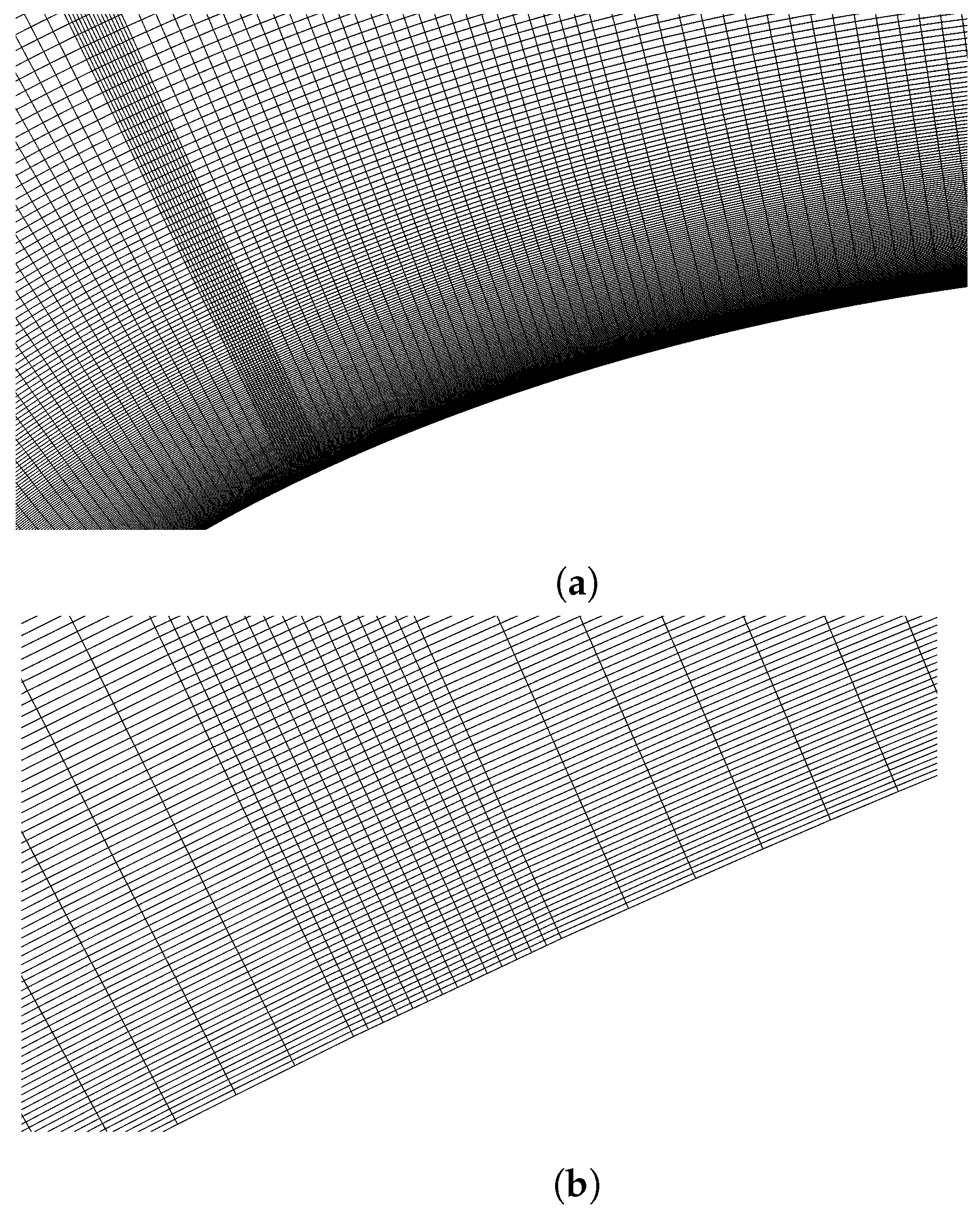
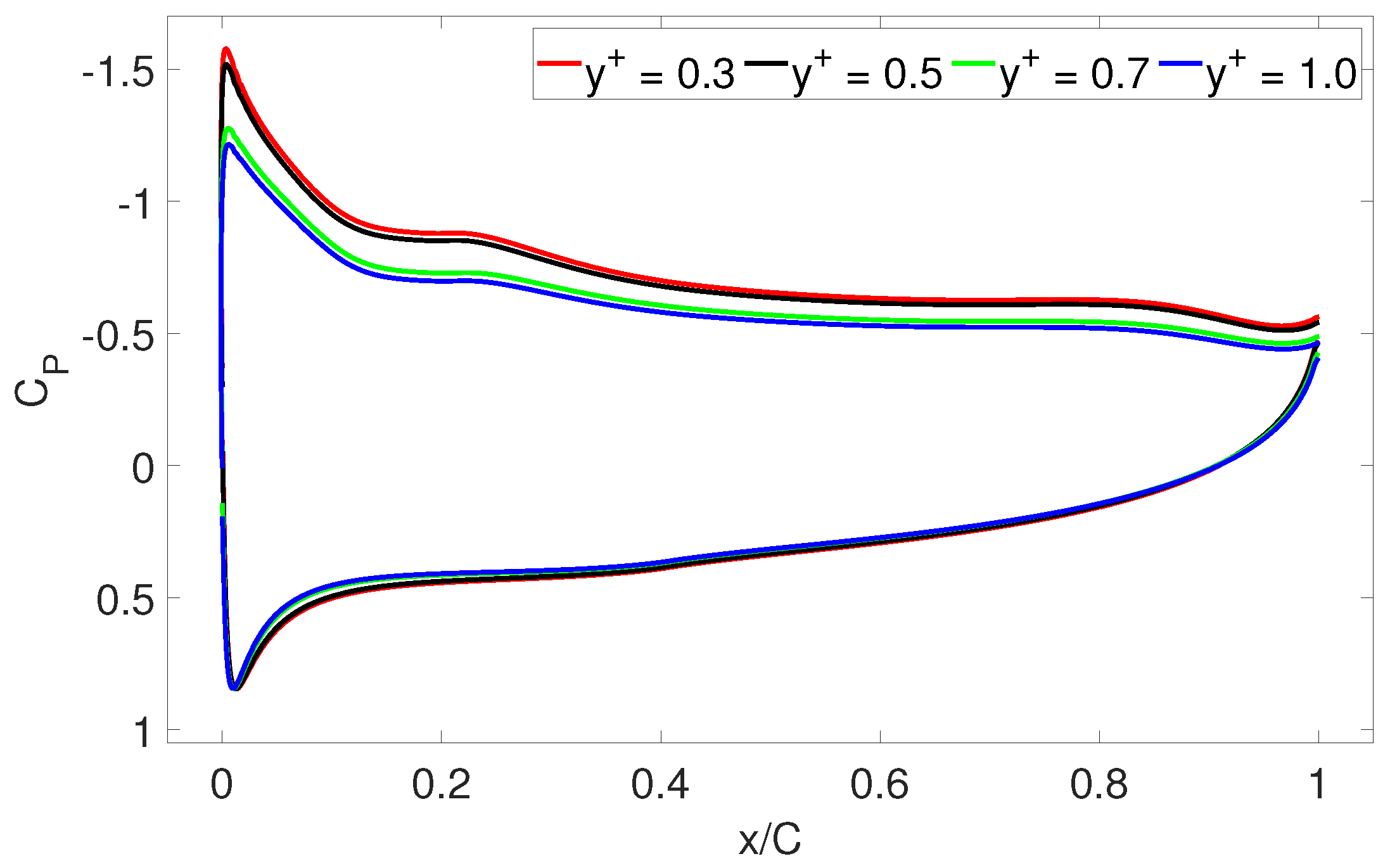
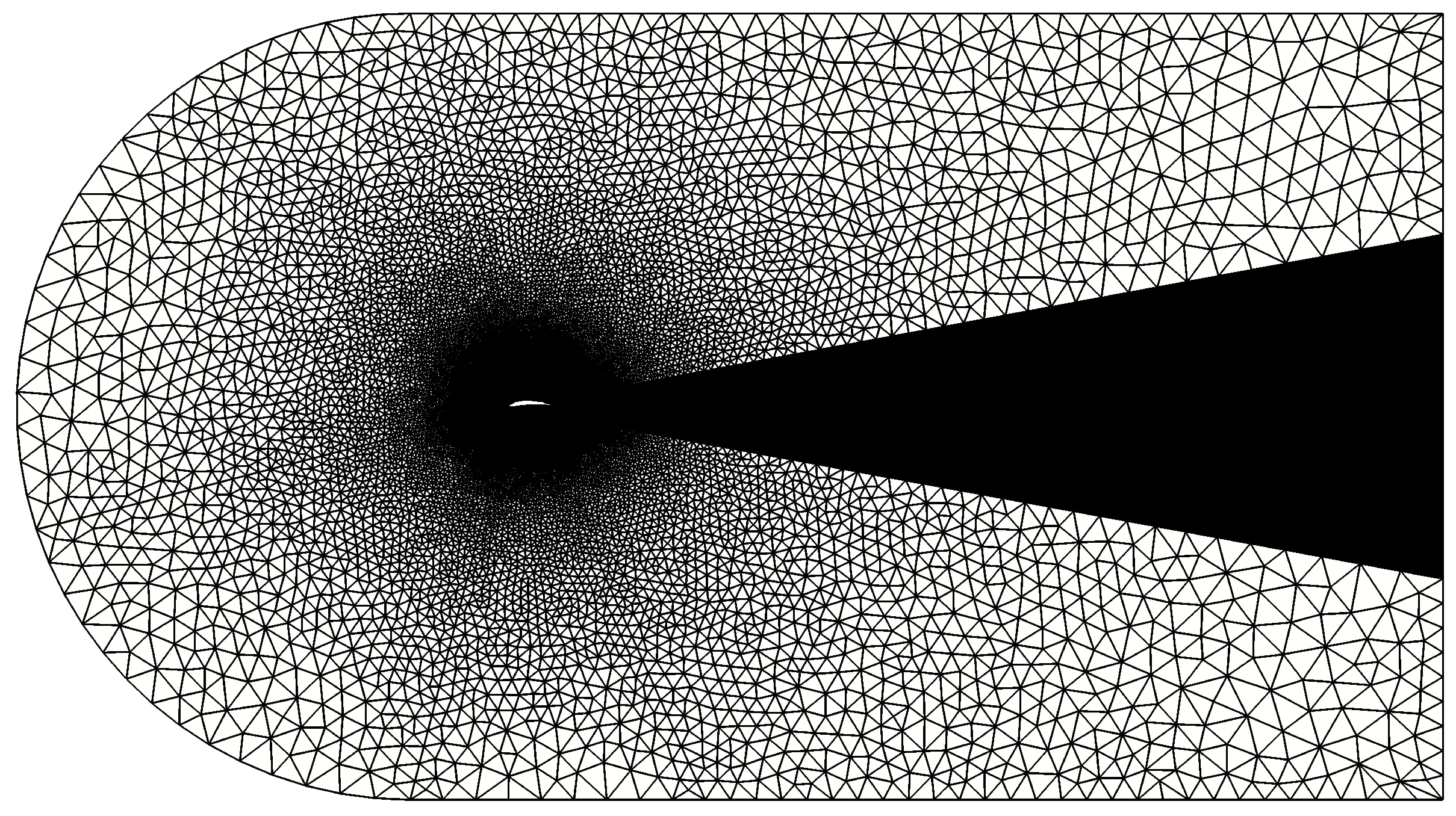
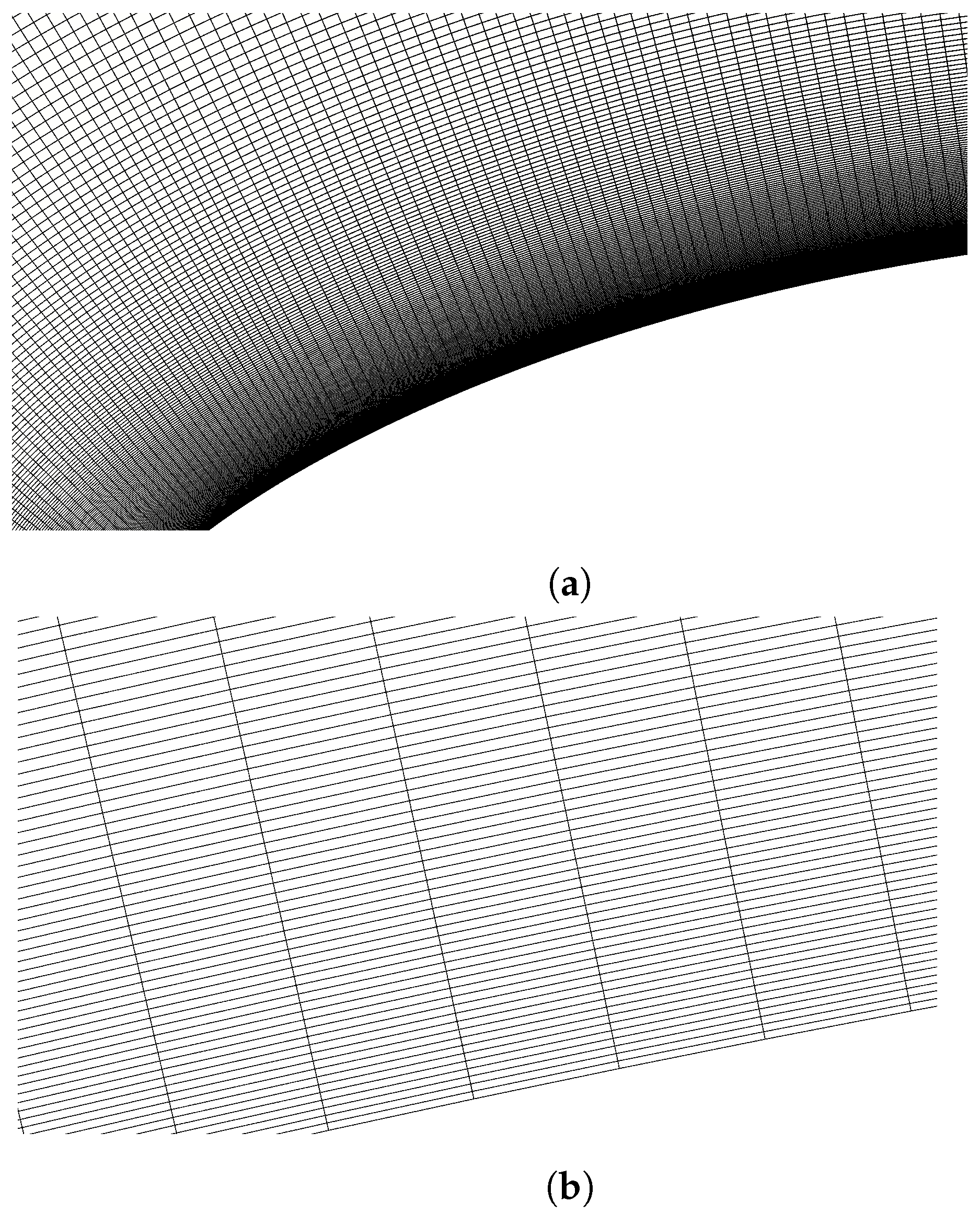
2.4. Mesh Assessment

Due to the fact that no previous experimental or numerical studies are available in the literature, it is essential to validate the numerical model. In order to study the baseline case and the later AFC configurations, a mesh independence test was performed to guarantee independence between the mesh resolution and the simulated results. A hybrid mesh configuration, composed by a rectangular structured and a triangular unstructured mesh region, was implemented in order to capture the boundary layer while saving computational power required on the outer regions of the domain. The surrounding region of the airfoil consists on two body-fitted structured sub-meshes with a progressive growth of 1% for the one closest to the airfoil and 3% for the one surrounding the first sub-mesh. The remaining portion of the domain was filled with an unstructured mesh, the resolution was particularly high on the wake region. An overall view of the computational domain is presented in Figure 3, a close up view of the regions surrounding the airfoil for the baseline case and for the corresponding AFC mesh implementation is shown in Figure 4 and Figure 5, respectively.

Four mesh candidates were designed according to four decreasing y⁺ values, and consequently an increasing mesh resolution, as it can be observed in

Table 2. Mesh candidates for the Mesh Independence Test.

${\mathit{y}}^{+}$	${\mathit{N}}_{\mathit{cell}}$	Cl	Cd	Cl$\mathit{Error}\%$	Cd$\mathit{Error}\%$	Calculated Maximum ${\mathit{y}}^{+}$
1	120,879	1.0797	0.2218	14.93	9.14	0.9127
0.7	139,551	1.1153	0.2267	12.12	7.13	0.6544
0.5	160,557	1.2267	0.2393	3.35	1.97	0.4728
0.3	183,897	1.2692	0.2441	-	-	0.2887

from the number of mesh cells $N_{cell}$ employed in the CFD models. Due to the lack of experimental data for the NACA-8412 airfoil at $Re=68.5\times {10}^3$, the evaluation of the proper mesh could not be based on the relative error between experimental and computational data. Alternatively, the strategy followed was to study the temporal averaged $C_l$ and $C_d$, as well as $C_P$ and $C_F$ distributions along the chord for each mesh candidate, and to compare them to observe for which y⁺ the results did not significantly change. This approach was also applied to evaluate whether the relative error between the results compensated in terms of computational cost. A baseline case simulation was performed for each mesh candidate for a computational time of 30 s, which was determined based on the evaluation of the velocity and pressure residuals. The time step was of $2\times {10}^{-4}$ s. In order to avoid the transient phase, the resulting time averaged for the lift $C_l$ and drag $C_d$ coefficients were computed considering the last 10 s of each simulation. The resulting averaged aerodynamic coefficients together with the relative error $C_{l}Error$, $C_{d}Error$ given in percentage are presented in Table 2. Calculated $y^{+}$ values were assessed on the upper side of the airfoil due to its importance in the later AFC implementation, and its maximum value obtained for each case is also included in Table 2. The resulting pressure and friction coefficients are introduced in Figure 6 and Figure 7, respectively.

Table 2 shows that the time averaged aerodynamic coefficients stabilize as $y^{+}$ decreases. For instance, the relative error between $y^{+}$ = 0.3 and $y^{+}$ = 1 is 14.93% for $C_l$ and 9.14% for $C_d$. On the other hand, the relative error between $y^{+}$ = 0.3 and $y^{+}$ = 0.5 is 3.35% for $C_l$ and 1.97% for $C_d$. As the difference among the aerodynamic coefficients for $y^{+}$ = 0.3 and $y^{+}$ = 0.5 can be considered relatively small ($\Delta C_l$ = −0.0425 and $\Delta C_d$ = $4.8\times {10}^{-3}$, with reference values corresponding to the $y^{+}$ = 0.3 results), and the computational time for the $y^{+}$ = 0.3 resulted in nearly the double than the one required for $y^{+}$ = 0.5, the results corresponding to the mesh with an estimated $y^{+}$ = 0.5 were considered acceptable for the present simulations. It is relevant to highlight that the calculated maximum $y^{+}$ values on the airfoil upper surface were slightly lower than the estimated ones used to determine the first cell height, which certifies that the mesh was properly designed and ensured the condition of $y^{+}<1$ necessary to evaluate the boundary layer.

In order to further check the mesh to be employed, the pressure coefficient $C_P$ evaluated at each point of the airfoil surface and for all $y^{+}$ studied is presented in Figure 6. The $C_P$ distribution along airfoil lower surface showed a very similar behaviour for every mesh candidate, despite that $y^{+}$ = 1 and $y^{+}$ = 0.7 showed a slightly lower $C_P$ value for approximately the 80% of the chord. A more notable difference can be observed in the airfoil upper surface, where $C_P$ progressively grows as $y^{+}$ decreases. It can be observed how $C_P$ in the airfoil upper surface for $y^{+}$ = 0.3 and $y^{+}$ = 0.5 are very similar along the whole chord, only showing a minor difference between the leading edge of the airfoil and $x/C$ = 0.3. When considering the friction coefficient, see Figure 7, no notable differences can be noticed between the $C_F$ distribution for the different meshes studied. The separation point is well predicted by all meshes evaluated, while small differences are observed in the reattachment point. After analyzing the $C_P$, $C_F$, $C_l$ and $C_d$ coefficients, we can conclude that the results obtained for the mesh with an estimated $y^{+}$ = 0.5 are representative and almost mesh independent. This mesh was selected for the baseline case evaluation as well as for the later AFC implementation simulations. In addition, selecting this mesh exploited the fact that the computational time required to complete the simulations was drastically lower than for the most dense mesh, without compromising the solution in a great extent. To conclude with the baseline case analysis, the streamlines of the averaged flow field are presented in Figure 8. A huge separation bubble is generated very close to the airfoil LE, as indicated in Figure 7, and it extends up to the vicinity of the TE, where a counter rotating vorticular structure is generated. Notice that the boundary layer separation point is observed to be at about $10\%$ of the chord, $x/C$ = 0.1045. The objective of the AFC implementation is to postpone the boundary layer separation, breaking this large vorticular structure onto smaller ones, or even completely suppressing it. This will reduce the drag generated by the large vortex and increase the lift generated by the airfoil.

3. AFC Implementation

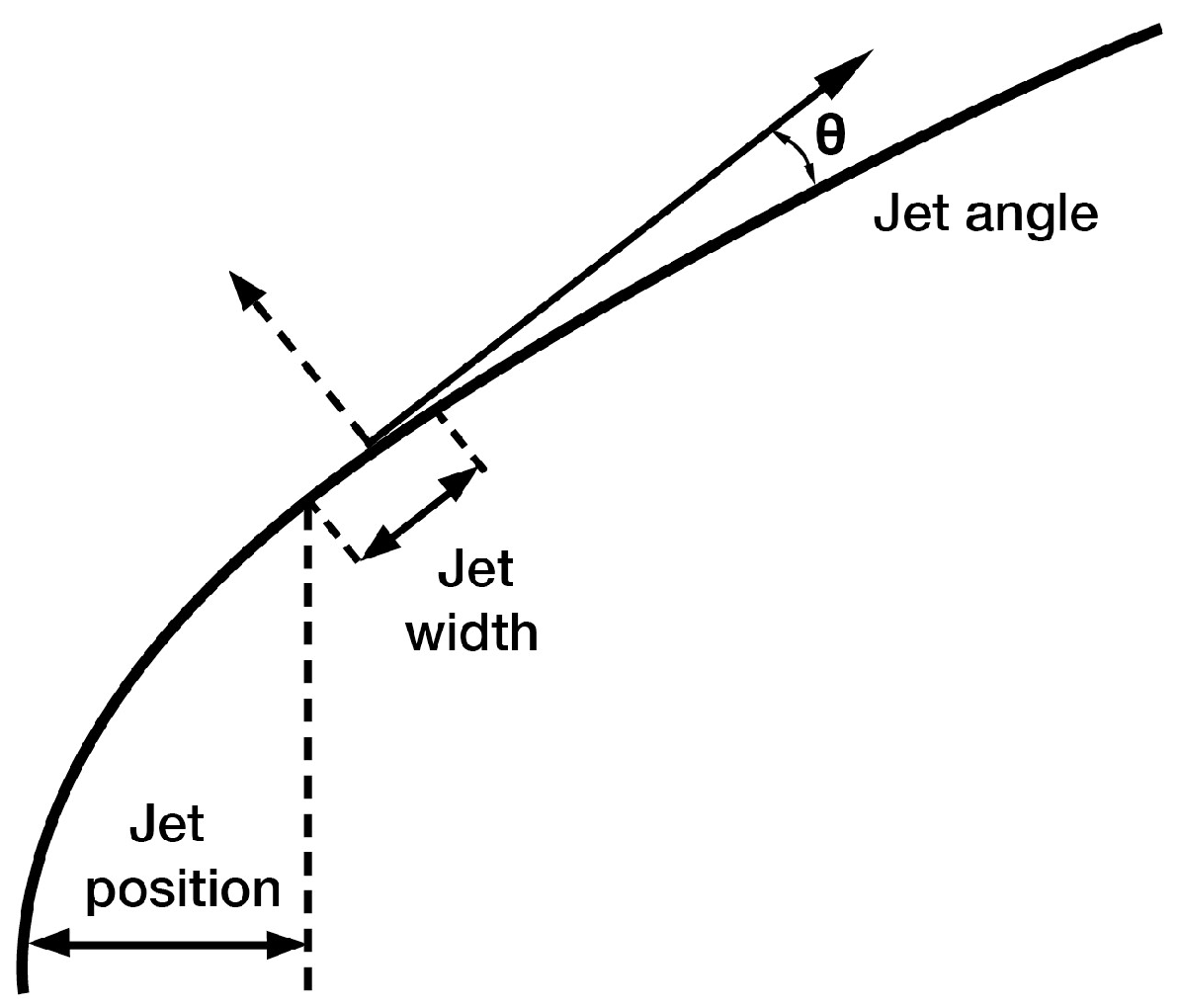
3.1. Jet Location and Mesh Modification

In order to evaluate the influence of AFC on aerodynamic efficiency, three design variables have been studied: the jet inclination angle $\theta$, the jet momentum coefficient $C_{\mu }$ and the non-dimensional forcing frequency $F_{*}^{+}$. In the present study, the groove width h and location were kept constant. The design of the AFC synthetic jet begins by studying its location over the airfoil. According to [33] among others, the optimum location is just upstream of the boundary layer separation point, which can clearly be seen in Figure 7 and Figure 8. The separation point is located at $x/C$ = 0.1045, considerably close to the LE. This is a consequence of the high AoA used (15°) and of the geometry of the airfoil selected, as it shows a pronounced curvature near the leading edge. At the separation point $C_F$ begins to adopt negative values due to the adverse pressure gradient, leading to flow separation. Based on what it was defined in reference [4], the synthetic jet has been placed at a location of 0.01C upstream of the flow separation point, with a slot width of 0.01C ($1\%$ of the chord), from $x/C$ = 0.08 to $x/C$ = 0.09. The next step is to design the AFC velocity signal, which must be time periodic as the jet corresponds to the ZNMF typology. Thus, in the following subsections, the frequency, amplitude and jet inclination angle will need to be evaluated. The mesh was further refined in the slot region due to the quick variation of the flow properties close to the jet. For this reason, the number of partitions at the vicinity of the jet have been increased as it can be seen in Figure 5. The total number of mesh cells increased to 162,789 for the cases where AFC was considered. Regarding the instantaneous velocity along the groove it was decided to use a top hat velocity distribution.

3.2. AFC Velocity Input

Synthetic jets, also called ZNMF actuators, are characterized by transporting the same quantity of fluid in the blowing and suction phases. For this reason, a sinusoidal velocity input as in Equation (23) must be designed with the objective of extracting and injecting moment from the boundary layer. An initial approach must be carried out to estimate a reference value for the velocity input frequency f and amplitude A.

$$U_{jet}\left(t\right)=A\sin \left(2\pi ft\right)$$

(23)

The introduction of periodic forcing is aimed to modify the airfoil vortex shedding frequency and amplitude. The vortex shedding natural frequency for the baseline case must be assessed by analyzing its frequency spectrum. Following the methodology presented in [37], a Fast Fourier Transform for the lift coefficient of the baseline case was performed. The resulting vortex shedding frequency was $f_0$ = 0.6965 Hz. The amplitude A of the velocity signal corresponds to the maximum velocity of the jet $U_{max}$ when sucked/injected from/to the boundary layer. The parametric study presented in this paper is designed as follows: the groove position and width were kept constant, and the natural vortex shedding frequency was selected as input frequency. Then, for a given jet inclination angle, CFD simulations were performed for a set of momentum coefficients $C_{\mu }$ ranging between $0.0001\le C_{\mu }\le 0.1$. The process was performed for three different jet inclination angles of $\theta$ = 20°, 30° and 40°. Via following this procedure the optimum momentum coefficient and jet injection angle (from the range chosen) were obtained. As a final step, a set of jet pulsating frequencies ranging between $0.5\le F_{*}^{+}\le 7$ were evaluated for the optimum $C_{\mu }$ and $\theta$ configuration previously obtained.

4. Results

Three jet inclination angles $\theta$ have been studied (20°, 30° and 40°). For each $\theta$, twelve momentum coefficients $C_{\mu }$ have been evaluated to obtain the optimal $\theta$ and $C_{\mu }$ configuration among those studied. The rest of the parameters were kept constant. The range of $C_{\mu }$ values have been selected based on previous validated studies [38].

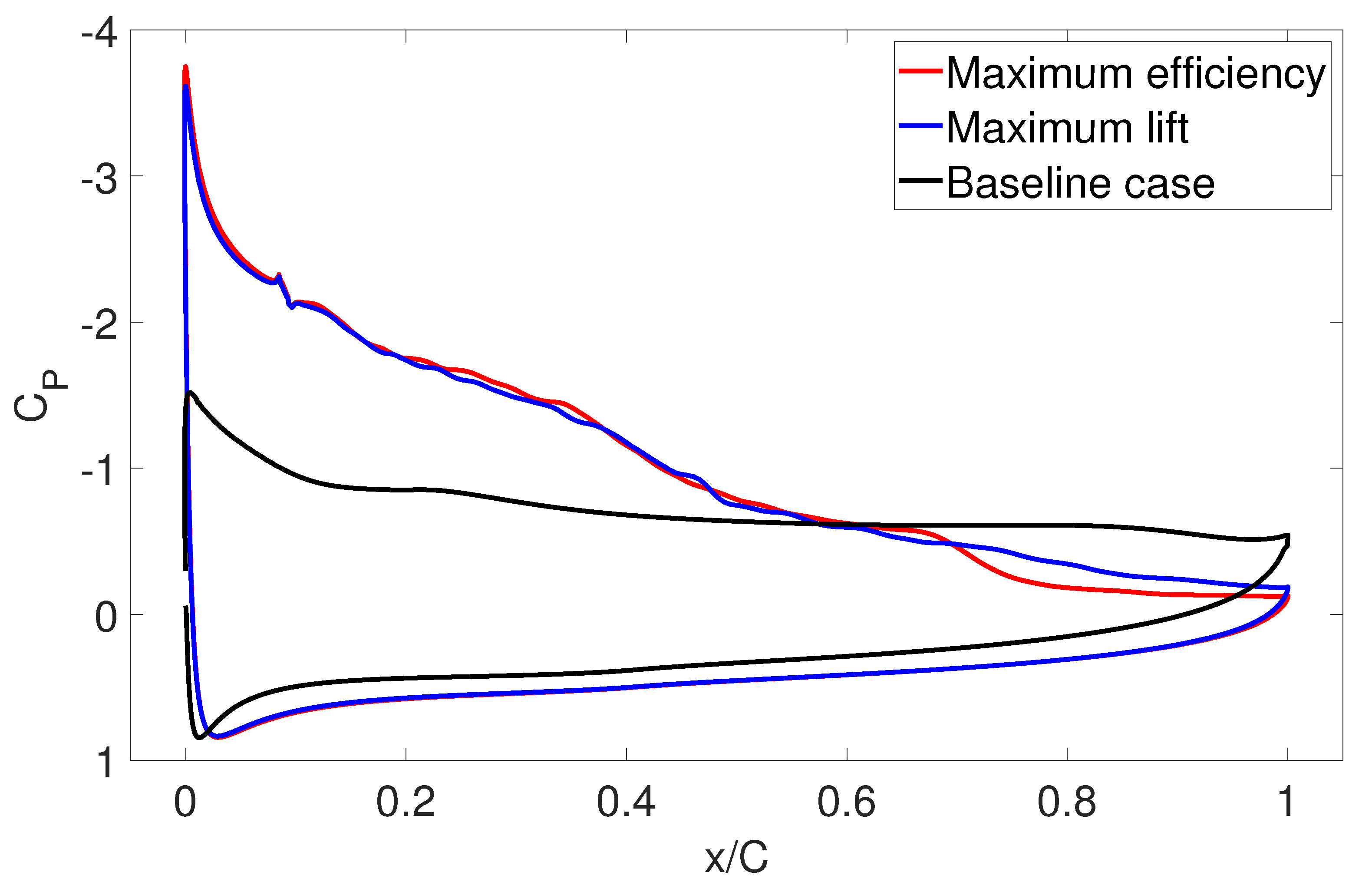
4.1. Optimal $\theta$ and $C_{\mu }$ Configuration

Figure 9 introduces the different values of the temporal averaged $C_l$, $C_d$ and aerodynamic efficiency $E=C_l/C_d$ as a function of the different jet injection angles $\theta$ and momentum coefficients $C_{\mu }$ studied. Observing Figure 9a, it can be stated that regardless of the injection angle studied, high $C_l$ are obtained for momentum coefficients ranging between $0.0005\le C_{\mu }\le 0.05$. In general the optimum jet inclination angle is $\theta$ = 40°, although two maximum lift coefficients are obtained at $\theta$ = 40° $C_{\mu }$ = 0.0005 and $\theta$ = 20° $C_{\mu }$ = 0.001, respectively. Regarding the results at $\theta$ = 30°, the graphic presents a much flatter shape than for $\theta$ = 20°, with an efficiency maximum at about $C_{\mu }$ = 0.005. In fact, regardless of the injection angle studied, the maximum lift coefficients are obtained for momentum coefficients in the range $0.0005\le C_{\mu }\le 0.001$.

For $C_{\mu }$ values larger than 0.015, regardless of the injection angle, the lift coefficient values significantly decrease. Finally, the $C_l$ curve obtained for $\theta$ = 40° is the most flat one, indicating the lift obtained at this inclination angle is good and pretty stable for a large range of momentum coefficients. Note that as $\theta$ increases, $C_l$ tends to be more stable in the range of $C_{\mu }$ between 0.0005 and 0.015, indicating that the effectiveness of $C_{\mu }$ is higher for growing $\theta$ values. When considering the drag coefficient in Figure 9b, minimum values are obtained for $\theta$ = 40°, although for $\theta$ = 30° relatively low drag coefficients are observed. The minimum $C_d$ is obtained at $\theta$ = 40° and $C_{\mu }$ = 0.003. Comparing Figure 9a with Figure 9b it can be concluded that to maximize lift and minimize drag the optimum jet injection angle is $\theta$ = 40°, yet, the momentum coefficient to maximize lift is $C_{\mu }$ = 0.0005 while the one minimizing drag needs to be $C_{\mu }$ = 0.003. In order to solve this dilemma the airfoil efficiency must be considered.

Airfoil efficiency E is presented in Figure 9c. Maximum aerodynamic efficiencies are obtained for $\theta$ = 40° followed by $\theta$ = 30°. The maximum aerodynamic efficiency has been obtained for $\theta$ = 40° and $C_{\mu }$ = 0.003, with E = 12.3291. Comparing this case with the baseline case, it supposes a $\Delta C_l$ = 0.51154, $\Delta C_d$ = −0.098, and $\Delta E$ = 7.2043. Consequently, these results have been considered satisfactory in order to proceed with the frequency study.

For completeness,

Table A1. AFC results comparison at different jet injection angles $\mathbf{\theta }$ and momentum coefficients ${\mathbf{C}}_{\mathbf{\mu }}$.

$\mathit{\theta }$	${\mathit{C}}_{\mathit{\mu }}$	${\mathit{C}}_{\mathit{l}}$	${\mathit{C}}_{\mathit{d}}$	E
-	-	1.2267	0.2393	5.1262
20°	0.0001	1.5059	0.2413	6.2408
	0.0005	1.7246	0.1746	9.8774
	0.0008	1.7390	0.1840	9.4511
	0.001	1.7704	0.1824	9.7061
	0.003	1.6925	0.1586	10.6715
	0.005	1.6823	0.1517	11.0897
	0.007	1.6877	0.1552	10.8744
	0.01	1.6893	0.1570	10.7599
	0.015	1.6828	0.1519	11.0783
	0.02	1.6642	0.1466	11.3520
	0.05	1.4941	0.1691	8.8356
	0.1	1.4470	0.1815	7.9725
30°	0.0001	1.5872	0.1904	8.3361
	0.0005	1.7310	0.1754	9.8689
	0.0008	1.7570	0.1791	9.8102
	0.001	1.7147	0.1485	11.5468
	0.003	1.7041	0.1478	11.5298
	0.005	1.7122	0.1451	11.8001
	0.007	1.7363	0.1634	10.6261
	0.01	1.7141	0.1609	10.6532
	0.015	1.7194	0.1587	10.8343
	0.02	1.6897	0.1556	10.8593
	0.05	1.6121	0.1523	10.5850
	0.1	1.5612	0.1791	8.7169
40°	0.0001	1.5957	0.1918	8.3196
	0.0005	1.7739	0.1764	10.0561
	0.0008	1.7415	0.1770	9.8390
	0.001	1.7587	0.1621	10.8495
	0.003	1.7421	0.1413	12.3291
	0.005	1.7273	0.1471	11.7424
	0.007	1.7309	0.1439	12.0285
	0.01	1.7304	0.1531	11.3024
	0.015	1.7439	0.1590	10.9679
	0.02	1.7128	0.1495	11.4569
	0.05	1.6810	0.1590	10.5723
	0.1	1.6031	0.1790	8.9559

is presented in Appendix A, where the results obtained from the different simulations previously introduced in Figure 9 are presented. Note that all values presented in this table correspond to the time averaged values obtained during the last 10 seconds of each simulation.

4.2. Forcing Frequency Analysis

As it has been previously mentioned, maintaining constant the groove position and width as well as the AFC parameters optimized in Section 4.1 ($\theta$ = 40° and $C_{\mu }$ = 0.003), a set of different $F_{*}^{+}$ values ($0.5\le F_{*}^{+}\le 7$) have been applied in the present subsection. After simulating each $F_{*}^{+}$ case for a computational time of 30 s, the resulting time averaged $C_l$ and $C_d$ values, as well as the airfoil efficiency are presented in

Table 3. Time averaged aerodynamic coefficients and efficiency obtained for the set of $F_{*}^{+}$ studied.

${\mathit{C}}_{\mathit{\mu }}$	${\mathit{F}}_{*}^{+}$	${\mathit{C}}_{\mathit{l}}$	${\mathit{C}}_{\mathit{d}}$	E
0.003	0.5	1.6473	0.2063	7.9853
	1	1.7421	0.1413	12.3331
	2	1.8075	0.1289	14.0214
	3	1.8272	0.1120	16.3160
	4	1.8147	0.0942	19.2649
	5	1.8220	0.1054	17.2829
	7	1.7724	0.1190	14.8941

. The optimum case corresponds to $F_{*}^{+}$ = 4, with a resulting $C_l$ = 1.8147, $C_d$ = 0.0942 and E = 19.2649. It can be concluded that the modification of the pulsating flow frequency has brought an efficiency improvement of around $56\%$ versus the one obtained with the optimum $C_{\mu }$ and $\theta$. The increase in lift and decrease in drag corresponds to $\Delta C_l$ = 0.0726 and $\Delta C_d$ = −0.0471, respectively. When comparing the final AFC optimum properties with the baseline case ones, it is observed an airfoil efficiency increase of $275.8\%$, being the lift increase and drag decrease respectively of $\Delta C_l$ = 0.588 and $\Delta C_d$ = −0.1451. From Table 3 there is another condition which is worth to report, this is the maximum lift condition, which happens for $F_{*}^{+}$ = 3. It is interesting to note that the AFC parameters to obtain maximum efficiency and maximum lift are almost the same, just the pulsating frequency is slightly different, being four times and three times the natural vortex shedding frequency, respectively.

The drastic increase in airfoil efficiency is clearly understood when observing the evolution of the pressure coefficient over the airfoil when the optimized AFC parameters are considered. In Figure 10, the pressure coefficient distribution along the chord is presented for the baseline, maximum efficiency and maximum lift cases. For both maximum conditions, a substantial increase of $C_P$ is observed along the airfoil. From $x/C$ = 0 up to $x/C$ = 0.6, a huge decrease of the pressure coefficient is seen on the airfoil upper surface, while on the last $40\%$ of the chord the pressure is a bit higher than the one obtained in the baseline case.

To further understand the flow structure around the airfoil, streamlines of the averaged flowfield for the maximum efficiency and maximum lift cases are presented in Figure 11a,b, respectively. A drastic reduction of the vorticular structure generated over the airfoil upper surface with respect to the baseline case solution (see Figure 8) can be observed for both configurations presented. Clearly, for the maximum efficiency condition vortical structures have nearly disappeared over the airfoil. Just a small laminar bubble which appears at about $x/C$ = 0.7 and disappears before $x/C$ = 0.8 can be observed, indicating a corresponding boundary layer separation and reattachment at these points. The separation of the boundary layer is delayed to about $x/C$ = 0.7 for the case of maximum lift, reattaching close to the trailing edge. An elongated vortical structure is therefore generated around the airfoil trailing edge.

A good method to understand the flow evolution over the airfoil is via plotting the boundary layer thickness along the airfoil chord. For the baseline, maximum efficiency and maximum lift cases, this is presented in non-dimensional form and every $10\%$ of the chord in Figure 12. The set of profiles for both the maximum efficiency and maximum lift cases show only positive velocity values up to around $x/C$ = 0.7, entitling no boundary layer separation appears until this streamwise position. For the maximum efficiency case, at around $x/C$ = 0.7, negative averaged velocities start appearing close to the wall, returning to a completely positive profile at $x/C\approxeq$ 0.8, which matches perfectly well with the small laminar bubble observed in Figure 11a. A slightly different behaviour is observed for the maximum lift case, where Figure 12 shows how the averaged velocities close to the wall become negative for the streamwise positions ranging from $x/C$ = 0.7 and $x/C$ = 1. A direct connection between the boundary layer thickness just presented and what it is observed in Figure 11b can be made, the elongated and downstream growing vortex is clearly observed in both figures. When observing the negative velocity distributions associated to the maximum lift case from Figure 12b, and when comparing them with the velocity distributions corresponding to the baseline case, it can be concluded that the intensity associated to the maximum lift case vortex is much smaller than the one corresponding to the baseline case, therefore the maximum lift vortex must rotate with a low angular velocity. The vortex generated for the maximum efficiency configuration at around $x/C$ = 0.7 has a larger vorticity magnitude than the maximum lift one, but still lower than the vorticity associated to the baseline case vortex. For the baseline case, negative averaged velocity values can be observed from the streamwise position $x/C$ = 0.1 up to $x/C$ = 1, indicating a rapid separation of the boundary layer that extends for the whole airfoil. In reality, the negative averaged velocities cannot be clearly seen at streamwise position $x/C$ = 0.1 in Figure 12a, but the separation point can be easily localized around $x/C$ = 0.1 in Figure 12a. At $x/C$ = 1, slightly positive averaged velocities can be observed close to the wall due to the appearance of a counter rotating vortex generated at the trailing edge, as observed in Figure 8.

4.3. Energy Assessment

In order to find out how effective is the AFC approach employed for the maximum efficiency and maximum lift cases, the power per unit length required by the SJA ($W_j$) as well as the power saved after the actuation ($W_G$) have to be calculated. The power needed to drive the synthetic jet is given as:

$$W_j=\frac{1}{2}{\rho }_j{S}_{j}sin\left(\theta \right)\overline{u_j^3}$$

(24)

where $S_j=h\ast l$ defines the groove cross-sectional area, due to the fact that the airfoil length is equal to unity l = 1, the groove and the the jet width h are equivalent. The parameter $\theta$ stands for the jet inclination angle measured versus the wing profile surface.

The definition of the synthetic jet actuator time dependent velocity profile to the power three, $\overline{u_j^3}$, was taken from [6,39].

$$\overline{u_j^3}=\frac{1}{T/2}{\int }_0^{T/2}{U_{max}}^3{sin}^3\left(2\pi ft\right)dt=\frac{4}{3\pi }{U_{max}}^3$$

(25)

where $U_{max}$ characterizes the jet maximum velocity. The equation representing the power saved when AFC is applied and due to the drag force reduction, takes the form:

$$W_G=U_{\infty }\left(D_{\mathrm{baseline}}-D_{\mathrm{actuated}}\right)=\frac{\rho {U_{\infty }}^{3}C}{2}\left(C_{d_{\mathrm{baseline}}}-C_{d_{\mathrm{actuated}}}\right)$$

(26)

where the drag force and the drag coefficient are respectively given as D and $C_d$. When AFC is applied, the parameter defining the power ratio $P_R$ is represented as:

$$P_R=\frac{W_G}{W_j}$$

(27)

Energy saving exist for power ratio values higher than one.

The set up parameters and resulting power ratios are summarised in

Table 4. Power ratio values characterizing the maximum efficiency and maximum lift configurations.

Cases	${\mathit{\alpha }}^{\circ }$	${\mathit{U}}_{\mathit{max}}$ [$\mathbf{m}/\mathbf{s}$]	${\mathit{S}}_{\mathit{j}}$ [${\mathbf{m}}^2$]	${\mathit{\theta }}^{\circ }$	${\mathit{W}}_{\mathit{j}}$ [W]	${\mathit{W}}_{\mathit{G}}$ [W]	${\mathit{W}}_{\mathit{G}}/{\mathit{W}}_{\mathit{j}}$
max efficiency	15	0.6832	0.01	40	5.3277 $\times {10}^{-4}$	0.0889	166.81
max lift	15	0.6832	0.01	40	5.3277 $\times {10}^{-4}$	0.0780	146.35

. Both maximum efficiency and maximum lift configurations present energy savings, with a power gain two orders of magnitude higher than the power required by the SJA.

This result confirms that the introduction of AFC in an airfoil with separated flow is capable of reducing the drag coefficient and increase the lift coefficient significantly, by keeping the boundary layer attached for a larger portion of the airfoil. Therefore, it can be sated that the implementation of the SJA is energetically efficient for the separated flow case presented.

5. Conclusions

This paper presents a parametric analysis on a NACA-8412 airfoil with the aim to optimize three AFC parameters, momentum coefficient, jet inclination angle and pulsating frequency, associated to a SJA. The procedure followed to perform a parametric optimization of any airfoil is established and presented. A maximum airfoil efficiency increase, measured respect to the baseline case, of $276\%$ is obtained for $C_{\mu }$ = 0.003; $F_{*}^{+}$ = 4 and $\theta$ = ${40}^{\circ }$, the groove was located from $x/C$ = 0.08 to $x/C$ = 0.09 being its width of $0.01C$. The maximum airfoil lift was obtained for the same AFC parameters except the pulsating frequency which was of $F_{*}^{+}$ = 3. The efficiency increase with respect to the baseline case was of around $218\%$. From the comparison of the AFC parameters for maximum lift and maximum efficiency cases, it is proved that the pulsating frequency is capable of highly improving the airfoil efficiency.

References

- Hochhäusler, D.; Erfort, G. Experimental study on an airfoil equipped with an active flow control element. Wind. Eng. 2021. [Google Scholar] [CrossRef]
- Khalil, K.; Asaro, S.; Bauknecht, A. Active flow control devices for wing load alleviation. J. Aircr. 2022, 59, 458–473. [Google Scholar] [CrossRef]
- Mosca, V.; Karpuk, S.; Sudhi, A.; Badrya, C.; Elham, A. Multidisciplinary design optimisation of a fully electric regional aircraft wing with active flow control technology. Aeronaut. J. 2021, 126, 730–754. [Google Scholar] [CrossRef]
- Tousi, N.M.; Coma, M.; Bergada, J.M.; Pons-Prats, J.; Mellibovsky, F.; Bugeda, G. Active Flow Control Optimisation on SD7003 Airfoil at Pre and Post-Stall Angles of Attack using Synthetic Jets. Appl. Math. Model. 2021, 98, 435–464. [Google Scholar] [CrossRef]
- Tadjfar, M.; Kamari, D. Optimization of Flow Control Parameters Over SD7003 Airfoil with Synthetic Jet Actuator. J. Fluids Eng. 2020, 142, 021206. [Google Scholar] [CrossRef]
- De Giorgi, M.; De Luca, C.; Ficarella, A.; Marra, F. Comparison between synthetic jets and continuous jets for active flow control: Application on a NACA 0015 and a compressor stator cascade. Aerosp. Sci. Technol. 2015, 43, 256–280. [Google Scholar] [CrossRef]
- Traficante, S.; De Giorgi, M.; Ficarella, A. Flow separation control on a compressor-stator cascade using plasma actuators and synthetic and continuous jets. J. Aerosp. Eng. 2016, 29, 04015056. [Google Scholar] [CrossRef]
- Zhang, H.; Chen, S.; Gong, Y.; Wang, S. A comparison of different unsteady flow control techniques in a highly loaded compressor cascade. Proc. Inst. Mech. Eng. Part G J. Aerosp. Eng. 2019, 233, 2051–2065. [Google Scholar] [CrossRef]
- Cattafesta, L.N.; Sheplak, M. Actuators for Active Flow Control. Annu. Rev. Fluid Mech. 2011, 43, 247–272. [Google Scholar] [CrossRef] [Green Version]
- Wang, L.; Tian, F.B. Numerical simulation of flow over a parallel cantilevered flag in the vicinity of a rigid wall. Phys. Rev. E 2019, 99, 053111. [Google Scholar] [CrossRef]
- Cho, Y.C.; Shyy, W. Adaptive flow control of low-Reynolds number aerodynamics using dielectric barrier discharge actuator. Prog. Aerosp. Sci. 2011, 47, 495–521. [Google Scholar] [CrossRef] [Green Version]
- Foshat, S. Numerical investigation of the effects of plasma actuator on separated laminar flows past an incident plate under ground effect. Aerosp. Sci. Technol. 2020, 98, 105646. [Google Scholar] [CrossRef]
- Benard, N.; Moreau, E. Electrical and mechanical characteristics of surface AC dielectric barrier discharge plasma actuators applied to airflow control. Exp. Fluids 2014, 55, 1846. [Google Scholar] [CrossRef] [Green Version]
- Benard, N.; Pons-Prats, J.; Periaux, J.; Bugeda, G.; Braud, P.; Bonnet, J.; Moreau, E. Turbulent separated shear flow control by surface plasma actuator: Experimental optimization by genetic algorithm approach. Exp. Fluids 2016, 57, 22. [Google Scholar] [CrossRef] [Green Version]
- Bergadà, J.M.; Baghaei, M.; Prakash, B.; Mellibovsky, F. Fluidic Oscillators, Feedback Channel Effect under Compressible Flow Conditions. Sensors 2021, 21, 5768. [Google Scholar] [CrossRef]
- Baghaei, M.; Bergada, J.M. Fluidic Oscillators, the Effect of Some Design Modifications. Appl. Sci. 2020, 10, 2105. [Google Scholar] [CrossRef] [Green Version]
- Baghaei, M.; Bergada, J.M. Analysis of the Forces Driving the Oscillations in 3D Fluidic Oscillators. Energies 2019, 12, 4720. [Google Scholar] [CrossRef] [Green Version]
- Glezer, A.; Amitay, M. Synthetic jets. Annu. Rev. Fluid Mech. 2002, 34, 503–529. [Google Scholar] [CrossRef]
- Rumsey, C.; Gatski, T.; Sellers, W.; Vatsa, V.; Viken, S. Summary of the 2004 CFD validation workshop on synthetic jets and turbulent separation control. In Proceedings of the 2nd AIAA Flow Control Conference, Portland, OR, USA, 28 June–1 July 2004; p. 2217. [Google Scholar]
- Wygnanski, I. The variables affecting the control of separation by periodic excitation. In Proceedings of the 2nd AIAA Flow Control Conference, Portland, OR, USA, 28 June–1 July 2004; p. 2505. [Google Scholar]
- Findanis, N.; Ahmed, N. The interaction of an asymmetrical localised synthetic jet on a side-supported sphere. J. Fluids Struct. 2008, 24, 1006–1020. [Google Scholar] [CrossRef]
- Amitay, M.; Smith, D.R.; Kibens, V.; Parekh, D.E.; Glezer, A. Aerodynamic flow control over an unconventional airfoil using synthetic jet actuators. AIAA J. 2001, 39, 361–370. [Google Scholar] [CrossRef]
- Amitay, M.; Glezer, A. Role of actuation frequency in controlled flow reattachment over a stalled airfoil. AIAA J. 2002, 40, 209–216. [Google Scholar] [CrossRef]
- Gilarranz, J.; Traub, L.; Rediniotis, O. A New Class of Synthetic Jet Actuators—Part I: Design, Fabrication and Bench Top Characterization. J. Fluids Eng. 2005, 127, 367–376. [Google Scholar] [CrossRef]
- You, D.; Moin, P. Active control of flow separation over an airfoil using synthetic jets. J. Fluids Struct. 2008, 24, 1349–1357. [Google Scholar] [CrossRef]
- Tuck, A.; Soria, J. Separation control on a NACA 0015 airfoil using a 2D micro ZNMF jet. Aircr. Eng. Aerosp. Technol. 2008, 80, 175–180. [Google Scholar] [CrossRef]
- Kitsios, V.; Cordier, L.; Bonnet, J.P.; Ooi, A.; Soria, J. On the coherent structures and stability properties of a leading-edge separated aerofoil with turbulent recirculation. J. Fluid Mech. 2011, 683, 395–416. [Google Scholar] [CrossRef]
- Buchmann, N.; Atkinson, C.; Soria, J. Influence of ZNMF jet flow control on the spatio-temporal flow structure over a NACA-0015 airfoil. Exp. Fluids 2013, 54, 1485. [Google Scholar] [CrossRef]
- Kim, S.H.; Kim, C. Separation control on NACA23012 using synthetic jet. Aerosp. Sci. Technol. 2009, 13, 172–182. [Google Scholar] [CrossRef]
- Monir, H.E.; Tadjfar, M.; Bakhtian, A. Tangential synthetic jets for separation control. J. Fluids Struct. 2014, 45, 50–65. [Google Scholar] [CrossRef]
- Goodfellow, S.D.; Yarusevych, S.; Sullivan, P.E. Momentum Coefficient as a Parameter for Aerodynamic Flow Control with Synthetic Jets. AIAA J. 2013, 51, 623–631. [Google Scholar] [CrossRef]
- Feero, M.A.; Goodfellow, S.D.; Lavoie, P.; Sullivan, P.E. Flow Reattachment Using Synthetic Jet Actuation on a Low-Reynolds-Number Airfoil. AIAA J. 2015, 53, 2005–2014. [Google Scholar] [CrossRef]
- Feero, M.A.; Lavoie, P.; Sullivan, P.E. Influence of synthetic jet location on active control of an airfoil at low Reynolds number. Exp. Fluids 2017, 58, 99. [Google Scholar] [CrossRef]
- Zhang, W.; Samtaney, R. A direct numerical simulation investigation of the synthetic jet frequency effects on separation control of low-Re flow past an airfoil. Phys. Fluids 2015, 27, 055101. [Google Scholar] [CrossRef] [Green Version]
- Rodriguez, I.; Lehmkuhl, O.; Borrell, R. Effects of the Actuation on the Boundary Layer of an Airfoil at Reynolds Number Re = 60000. Flow Turbul. Combust. 2020, 105, 607–626. [Google Scholar] [CrossRef]
- Spalart, P.; Allmaras, S. A one-equation turbulence model for aerodynamic flows. In Proceedings of the 30th Aerospace Sciences Meeting and Exhibit, Reno, NV, USA, 6–9 January 1992; p. 439. [Google Scholar] [CrossRef]
- Minelli, G.; Krajnovic, S.; Basara, B. Numerical Investigation of Active Flow Control Around a Generic Truck A-Pillar. Flow Turbul. Combust. 2016, 97, 1235–1254. [Google Scholar] [CrossRef] [PubMed] [Green Version]
- Tuck, A.; Soria, J. Active flow control over a NACA 0015 airfoil using a ZNMF jet. In Proceedings of the 15th Australasian Fluid Mechanics Conference, Sydney, Australia, 13–17 December 2004; pp. 13–17. [Google Scholar]
- De Giorgi, M.G.; Traficante, S.; De Luca, C.; Bello, D.; Ficarella, A. Active flow control techniques on a stator compressor cascade: A comparison between synthetic jet and plasma actuators. In Proceedings of the ASME Turbo Expo 2012: Turbine Technical Conference and Exposition, Copenhagen, Denmark, 11–15 June 2012; American Society of Mechanical Engineers: New York, NY, USA, 2012; Volume 44748, pp. 439–450. [Google Scholar]