An Efficient Hybrid Evolutionary Optimization Method Coupling Cultural Algorithm with Genetic Algorithms and Its Application to Aerodynamic Shape Design

Abstract

Evolutionary algorithms have been widely used to solve complex engineering optimization problems with large search spaces and nonlinearity. Both cultural algorithm (CA) and genetic algorithms (GAs) have a broad prospect in the optimization field. The traditional CA has poor precision in solving complex engineering optimization problems and easily falls into local optima. An efficient hybrid evolutionary optimization method coupling CA with GAs (HCGA) is proposed in this paper. HCGA reconstructs the cultural framework, which uses three kinds of knowledge to build the belief space, and the GAs are used as an evolutionary model for the population space. In addition, a knowledge-guided t-mutation operator is developed to dynamically adjust the mutation step and introduced into the influence function. HCGA achieves a balance between exploitation and exploration through the above strategies, and thus effectively avoids falling into local optima and improves the optimization efficiency. Numerical experiments and comparisons with several benchmark functions show that the proposed HCGA significantly outperforms the other compared algorithms in terms of comprehensive performance, especially for high-dimensional problems. HCGA is further applied to aerodynamic optimization design, with the wing cruise factor being improved by 23.21%, demonstrating that HCGA is an efficient optimization algorithm with potential applications in aerodynamic optimization design.

1. Introduction

Aircraft shape optimization is one of the key problems in aerodynamic configuration design. The traditional aerodynamic optimization design methods mainly rely on experience and trial-and-error methods, which require a lot of human, material and financial resources, and not only take a long time but also require a lot of computational resources [1]. In recent years, with the rapid development of computational fluid dynamics (CFD) technology, the combination of numerical methods and optimization algorithms for the aerodynamic shape optimization of aircraft can significantly shorten the development cycle and reduce the design cost [2]. Therefore, it is important to carry out research on efficient aerodynamic optimization design methods based on the combination of CFD technology and optimization algorithms for the development of aerodynamic optimization design.

Among numerous aerodynamic optimization studies, gradient-based methods and heuristic algorithms are two of the most widely used methods. Gradient-based methods are particularly attractive due to their ability to significantly improve the efficiency of high-dimensional optimization problems. The adjoint method proposed by Jameson [3] is an effective sensitivity analysis method that evaluates sensitivity information by solving the adjoint problem regardless of the number of design variables. Therefore, the computational time of sensitivity analysis can be significantly reduced. By combining the adjoint method with the gradient method, the optimization efficiency can be greatly improved. In recent years, this technique has been widely used in aerodynamic optimization [4,5]. However, two reasons make this technique less attractive: one is its difficulty in dealing with constrained/multi-objective problems, and the other is that it is easy for it to fall into local optima.

Heuristic algorithms do not need to rely on information about a specific problem and have good global performance in finding the optima; they are thus particularly suitable for solving problems with complex multiple local optima. Among them, genetic algorithms (GAs), differential evolution (DE) algorithm and particle swarm optimization (PSO) algorithm are the most popular methods in the field of aerodynamic optimization, and they have all been successfully applied in aerodynamic optimization [6,7,8,9]. However, their evolutionary procedures require multiple calls to the CFD analysers, which significantly increases the computational cost. Therefore, it is necessary to improve the optimal efficiency and therefore to develop optimization algorithms in particular allowing for balanced exploitation and exploration capabilities [10].

Many engineering problems are complex high-dimensional multimodal problems, so that most algorithms converge slowly, easily fall into local optima and are inefficient in dealing with such problems. Aerodynamic optimization is a highly complex nonlinear problem with multi-parameter, high-dimensional and multimodal characteristics. In order to solve aerodynamic optimization problems effectively, it is undoubtedly necessary to develop new intelligent and knowledge-based algorithms with satisfactory performance. The genetic algorithm has good robustness and global search capability [11,12,13,14,15], and can be well adapted to solve various types of problems. The cultural algorithm is a knowledge-based super-heuristic algorithm, and its unique two-layer evolutionary mechanism can improve the evolutionary efficiency very well. The hybrid of genetic algorithms and cultural algorithm can combine the advantages of both, and then solve aerodynamic optimization problems efficiently.

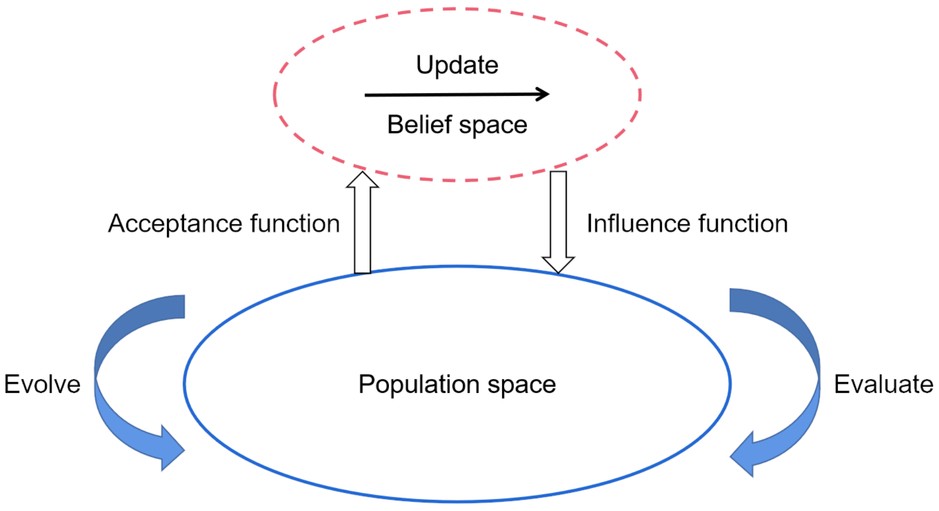
Cultural algorithm (CA) [16] is an evolutionary algorithm based on the simulation of a two-layer evolutionary mechanism of human society, proposed by R.G. Reynolds in 1994. It was inspired by and developed from human sociology and aimed to model the evolution of the cultural component of evolutionary systems over time [17]. CA simulates the development of society and culture, which can be divided into two parts, the population space and the belief space, which are independent from each other but interconnected through communication protocols. CA extracts the implicit information carried by the population evolution process, such as the location of the optimal individuals or the range of the best individuals, into the belief space and stores it in knowledge sources. CA provides a new framework and mechanism for evolutionary models or swarm intelligence systems [18], such as genetic algorithms [19], ant colony algorithms [20], particle swarm algorithms [21] and differential evolution [22], etc. The two-layer evolutionary mechanism of CA improves the efficiency of the algorithm. Compared with other evolutionary algorithms, CA has stronger global optimization capability and higher optimization precision, and it has been successfully applied to optimization problems such as clustering analysis [23], sensor localization [24], multi-objective optimization [25] and vehicle routing [26]. Although the cultural algorithm can use knowledge sources to improve evolutionary efficiency, its global convergence and evolutionary efficiency are deficient due to its single mutation operator [27]. Therefore, the cultural algorithm needs to be improved for better performance of the optimization.

In this paper, an efficient hybrid evolutionary optimization method coupling CA with GAs (HCGA) is introduced with a validation background of the application of evolutionary algorithms to aerodynamic optimization design. Considering the features of CA and GAs, the proposed algorithm reconstructs the framework of cultural algorithms, which uses GAs as a population space evolutionary model of the cultural framework, with the three types of knowledge, namely situational knowledge, normative knowledge and historical knowledge; these kinds of knowledge construct the knowledge sources of the belief space. In addition, HCGA introduces population variance and population entropy to determine population diversity, and it develops a new knowledge-guided t-mutation operator to dynamically adjust the mutation step based on the change of population diversity during the evolutionary process. It further introduces the t-mutation operator into the influence function to balance the exploration and exploitation ability of the algorithm and improve its optimization efficiency.

The rest of the paper is organized as follows. A brief introduction to the basic principles and framework of the cultural and genetic algorithms is given in Section 2. The proposed algorithm HCGA is introduced in Section 3. Numerical results and comparisons are presented and discussed in Section 4.2. The HCGA is applied in Section 5 to the aerodynamic optimization design of the wing cruise factor. Conclusions and perspectives are discussed in Section 6.

2. Brief Description of GAs and CA

2.1. Genetic Algorithms (GAs)

Genetic algorithms (GAs) proposed by Professor J. Holland [19] are among the evolutionary algorithms (EAs). GAs operate on the whole population with individuals, and their main operators include selection, crossover and mutation. For a particular problem, GAs define the search space as the solution space, and each feasible solution is encoded as a chromosome. Before the search starts, a set of chromosomes is usually randomly selected from the solution space to form the initial population. Next, the fitness value of each individual is evaluated according to the objective function, then the selection, crossover and mutation operators are applied sequentially to generate a new generation of populations. The process is repeated until the stopping criterion is reached.

2.2. Cultural Algorithm (CA)

The two-layer evolutionary mechanism used by the cultural algorithm consists of two main evolutionary spaces at the micro and macro levels, namely the population space and the belief space [28], and the basic structure of the cultural algorithm is shown in Figure 1. The evolution on the micro level refers to the internal evolution of the population space that realizes the evolution of individuals, and the evolution on the macro level refers to the evolution of the belief space that realizes the extraction and updating of knowledge sources. The evolutions between these two spaces are independent of each other, but they are connected through communication protocols (influence and acceptance functions). Figure 2 describes the basic pseudo-code of the CA. The figure shows how the process is executed in each generation. Firstly, the objective function Obj() evaluates individuals in the population space, and the Acceptance() function selects the best individuals for updating the belief space knowledge source. After that, the Influence() function influences the evolution of the next generation of populations. More details on the knowledge sources used and how they affect the population of this proposed work are given in Section 3.

3. The Hybrid Evolutionary Optimization Method Coupling CA with GAs

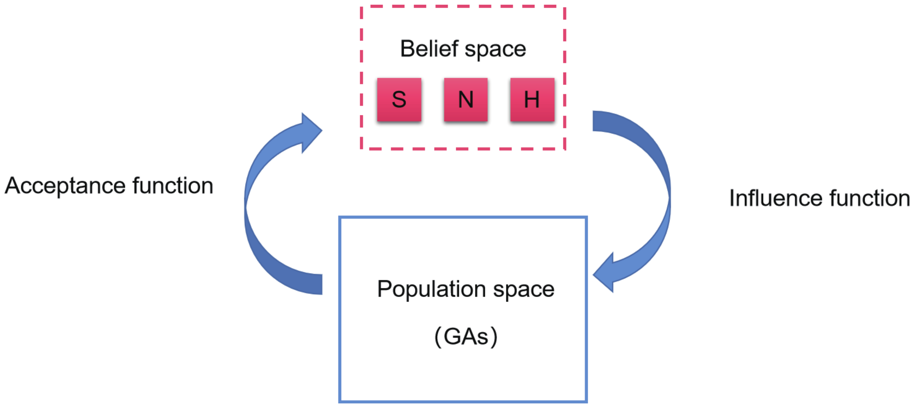
Cultural systems possess the ability to incorporate heterogeneous and diverse knowledge sources into their structures. As such, they are ideal frameworks within which to support hybrid amalgams of knowledge sources and population components [29]. In order to make full use of the advantages of CA and GAs, an efficient hybrid evolutionary optimization method coupling CA with GAs (HCGA) is proposed in this paper. The cultural framework of HCGA is shown in Figure 3, which includes population space, belief space and communication protocol, whose population space is modeled using GAs, and belief space includes situational knowledge, normative knowledge and historical knowledge. In addition, HCGA introduces population entropy and population variance to judge population diversity, and a knowledge-guided t-mutation operator is developed based on population diversity to balance the exploration and exploitation ability of the algorithm. In the remainder of this section, we describe each part of the HCGA in detail.

3.1. Population Space

In fact, the population space can support any population-based evolutionary algorithm or swarm intelligence algorithm, which can also interact and run simultaneously with the belief space. The standard cultural algorithm has only a single mutation operator in the population space, making its global convergence and exploration capability insufficient. The GAs has a strong global search capability and high robustness, which can effectively explore the search space with the increasing population convenience and global exploration capability of the algorithm, and thus the population space is evolved using the GAs in this paper. A detailed description of the genetic algorithms is given in Section 2.2 and will not be repeated here.

3.2. Belief Space

In this paper, according to the characteristics of genetic algorithms, combined with the manner of extracting and updating knowledge sources in the belief space, the knowledge sources are divided into situational knowledge, normative knowledge and historical knowledge. The manner of updating the knowledge sources in the belief space every K generations is adopted, so that the memory consumption brought by redundant information can be reduced. Different knowledge sources have different update strategies. Taking the maximization problem as an example, the update of the knowledge sources is described as follows:

(1)

Situational knowledge. Situational knowledge was proposed by Chung in 1997 [30] to record the excellent individuals with a guiding role in the evolutionary process and is structured as follows:

$$<E_1,E_2,\dots ,E_n>$$

(1)

where $E_i$ is the ith best individual, and in this paper the best individual is selected to update the situational knowledge, that is, s = 1. The process of updating situational knowledge is described as follows:

$$<E(T+1)>=\left\{\begin{array}{cc}<x_b>\hfill & \mathrm{if}f\left(x_b\right)>f\left(E\left(T\right)\right)\hfill \\ <E\left(T\right)>\hfill & \mathrm{else}\hfill \end{array}\right.$$

(2)

where $x_b$ is the best individual in the Tth generation of the population space.

(2)

Normative knowledge. Normative knowledge was also proposed by Chung [30] for limiting the search space and judging the feasibility of an individual. When an individual is outside the search space described by the normative knowledge, the normative knowledge will guide the individual into the dominant search space through the influence function, thus ensuring that evolution proceeds is in the dominant region, and for the n-dimensional optimization problem, the structure of the normative knowledge is described as follows:

$$<V_1,V_2,\dots ,V_n>$$

(3)

where $V_i=[(l_i,u_i),(L_i,U_i)],i\le n$. $u_i$ and $l_i$ are the upper and lower bounds of the ith dimensional variables, and $U_i$ and $L_i$ are the upper and lower bounds of the fitness value, respectively. The normative knowledge is updated with the change of the dominant search region, and gradually approaches the region where the best individual is located. Therefore, when there is a better individual in the Tth generation beyond the current search range described by the normative knowledge, the normative knowledge is updated as follows:

$$l_i(T+1)=\left\{\begin{array}{cc}{x}_j^i\left(T\right)\hfill & \mathrm{if}{x}_j^i\left(T\right)\le l_i\left(T\right))\mathrm{or}f\left(x_j\left(T\right)\right)>L_i\left(T\right)\hfill \\ l_i\left(T\right)\hfill & \mathrm{otherwise}\hfill \end{array}\right.$$

(4)

$$L_i(T+1)=\left\{\begin{array}{cc}f\left(x_j\left(T\right)\right)\hfill & \mathrm{if}{x}_j^i\left(T\right)\le l_i\left(T\right))\mathrm{or}f\left(x_j\left(T\right)\right)>L_i\left(T\right)\hfill \\ L_i\left(T\right)\hfill & \mathrm{otherwise}\hfill \end{array}\right.$$

(5)

$$u_i(T+1)=\left\{\begin{array}{cc}{x}_j^i\left(T\right)\hfill & \mathrm{if}{x}_j^i\left(T\right)\ge u_i\left(T\right))\mathrm{or}f\left(x_j\left(T\right)\right)>U_i\left(T\right)\hfill \\ u_i\left(T\right)\hfill & \mathrm{otherwise}\hfill \end{array}\right.$$

(6)

$$U_i(T+1)=\left\{\begin{array}{cc}f\left(x_j\left(T\right)\right)\hfill & \mathrm{if}{x}_j^i\left(T\right)\ge u_i\left(T\right))\mathrm{or}f\left(x_j\left(T\right)\right)>U_i\left(T\right)\hfill \\ U_i\left(T\right)\hfill & \mathrm{otherwise}\hfill \end{array}\right.$$

(7)

(3)

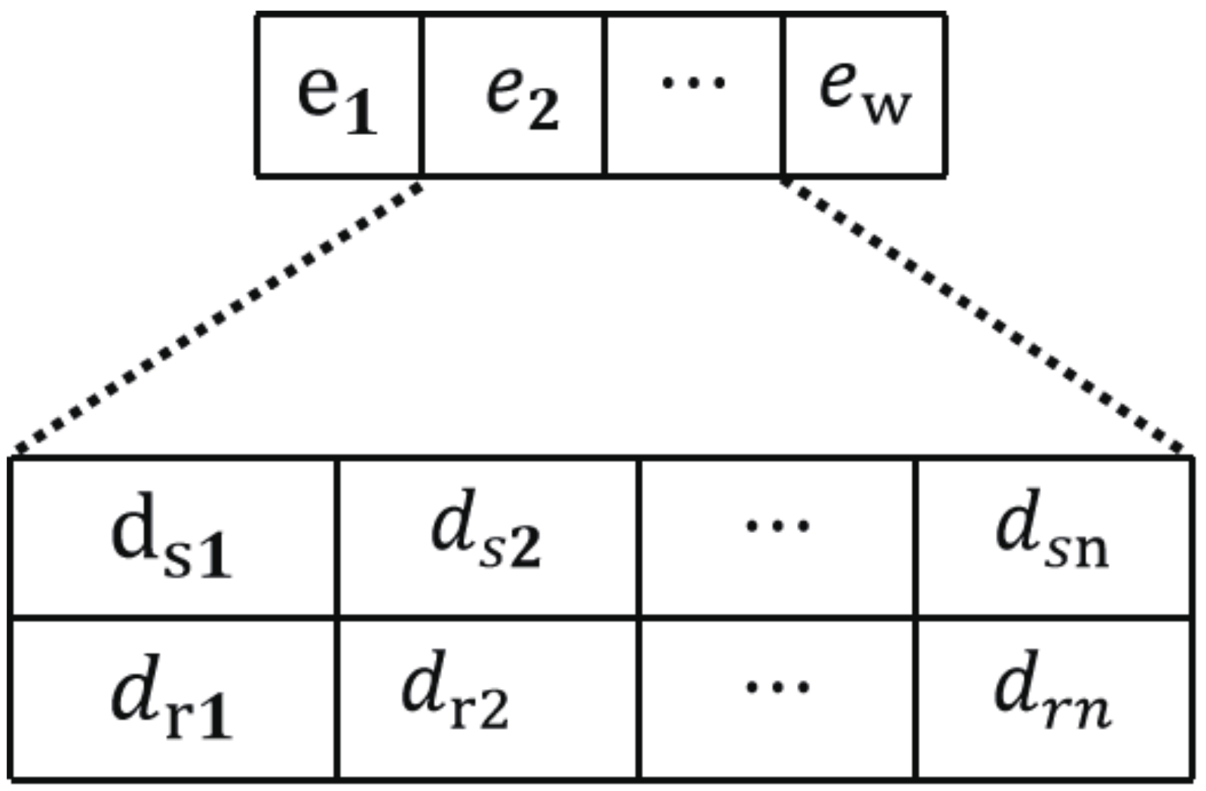
Historical knowledge. Historical knowledge was introduced into the belief space by Saleem [31] to record important events that occurred during the evolutionary process, and its main role is to adjust the offset distance and direction when the optimization falls into a local optima. The historical knowledge structure is divided as shown in Figure 4, where $e_i$ is the ith outstanding individual of historical knowledge preservation, W is its maximum capacity, and $d_{sj}$ and $d_{rj}$ are the average offset distance and the average offset direction of the jth design variable. The expressions of $d_{sj}$ and $d_{rj}$ are as follows:

$$d_{sj}=\frac{{\displaystyle \sum _{k=1}^{w-1}}|e_{k+1}{x}_j-e_k{x}_j|}{w-1}$$

(8)

$$d_{rj}=sgn\left(\sum _{k=1}^{w-1}|e_{k+1}{x}_j-e_k{x}_j|\right)$$

(9)

3.3. Proposed t-Mutation Operator

Evolutionary algorithms require good exploration capabilities in the early stages and good exploitation capabilities in the later stages of evolution. The t distribution contains the degree of freedom parameter n, which approaches the standard Gaussian distribution infinitely when $n\to +\infty$ and the t distribution is the standard Cauchy distribution when $n=1$. That is, the standard Gaussian distribution and the standard Cauchy distribution are two boundary special cases of the t distribution. The probability density functions of the standard Gaussian distribution and the standard Cauchy distribution are shown in Figure 5. Obviously, the application of the Cauchy operator can produce a larger mutation step, which is conducive to the algorithm to guide individuals to jump out of the local optimal solution and ensure the exploration ability of the algorithm, and Gaussian distribution shows a better exploitation ability.

Population diversity is considered as the primary reason for premature convergence, which determines the search capability of the algorithm. In evolutionary algorithms, population diversity decreases over time as evolution proceeds. Therefore, population diversity can be used to determine the stage of evolution; we can thus use the population diversity to construct the degree of freedom n. By changing the degree of freedom parameter n, the mutation scale changes adaptively with evolution to balance the exploitation and exploration capabilities of the algorithm. In this paper, we introduce population variance and population entropy to determine population diversity. The expression of population variance $D_T$ in the Tth generation is as follows:

$$D_T=\frac{1}{N\times l}\left(\sum _{i=1}^N\sum _{j=1}^l{x}_i^j-\overline{x^j}\right)$$

(10)

where $x_i^j$ is the jth gene value of the ith individual, N is the number of populations and l is the individual coding length. The expression of $\overline{x^j}$ is as follows:

$$\overline{x^j}=\frac{1}{N}\left(\sum _{i=1}^N{x}_i^j\right)$$

(11)

The solution space A of the optimization problem is divided equally into L small spaces, and the number of individuals belonging to the ith space $A_i$ in generation T is $|A_i|$. The expression of population entropy $S_T$ in the Tth generation is as follows:

$$S_T=-\sum _{i=1}^L{p}_{i}log\left(p_i\right)$$

(12)

where

$$p_i=\frac{|A_i|}{N}$$

(13)

From the definitions of population variance and population entropy, it is clear that population variance reflects the degree of dispersion of individuals in the population and that population entropy reflects the number of individual types in the population. Therefore, the t-mutation operator $t\left(n\right)$ can be constructed based on the population variance and population entropy. The degree of freedom parameter n is expressed as follows:

$$n=\left[1-ln\left(\frac{D_T+S_T}{D_{max}+S_{max}}\right)\right]$$

(14)

where $\left[\right]$ is the least integer function, and $D_{max}$ and $S_{max}$ are the maximum values of population variance and population entropy, respectively. Obviously, the degree of freedom parameter n of the t-mutation operator is 1 in the first generation and increases gradually as evolution proceeds, then the degree of freedom parameter n converges to positive infinity in the late evolutionary stage, and the t distribution becomes a standard Gaussian distribution. The t-mutation operator can ensure the exploration capability of the algorithm in the early evolutionary stage and the exploitation capability of the algorithm in the late evolutionary stage.

3.4. Communication Protocol

The information interaction between the belief space and the population space is realized through the acceptance function and the influence function. The acceptance function passes the better individuals in the population space as samples to the belief space for knowledge sources extraction and update, and the influence function is the way to influence the population space by the belief space, which can use the knowledge sources in the belief space to guide the population space to complete and accelerate the evolution.

3.4.1. Acceptance Function

In this paper, a dynamic version of the acceptance function [31] is used. The number of accepted individuals is given as follows:

$$n_{Accept}=\left(p\%+\frac{p\%}{T}\right)\times N$$

(15)

where $\left[\right]$ is the least integer function, T is the current generation, N is the number of populations, $p\%$ is the preset fixed proportion and $p\%=20\%$. In this paper, the acceptance function accepts $n_{Accept}$ better individuals into the belief space. The dynamic acceptance function makes the number of individuals entering the belief space decrease with the depth of evolution, which increases the global search ability of the algorithm at the early stage of evolution, and reduces the number of individuals entering the belief space at the late stage of evolution because the population tends to converge and carries mostly similar information, which can maintain the diversity of knowledge sources and avoid the consumption of memory by redundant information.

3.4.2. Influence Function

The core of the influence function is the manner and proportion in which each type of knowledge affects the population. Knowledge acts on each type of influence function to control the number of individuals affected by each type of influence function. Therefore, the proportion by which each type of knowledge affects the population is the relative role that each type of influence function has in the population. The proportion of the effect of the influence function is determined by the success rate of the knowledge effect, and is expressed as follows:

$$P_k\left(T\right)=\left\{\begin{array}{cc}1/N_k\hfill & \mathrm{if}T=1\hfill \\ \alpha +\beta \times \frac{v_k(T-1)}{v(T-1)}\hfill & \mathrm{if}\left(TmodK\right)=0\hfill \\ P_k(T-1)\hfill & \mathrm{otherwise}\hfill \end{array}\right.$$

(16)

It satisfies the condition that $\beta +\alpha \times N_k=1$, where $N_k$ is the number of knowledge sources types, $v_k(T-1)$ denotes the number of individuals influenced by knowledge k that are better than their parents in generation $T-1$ and $v(T-1)$ denotes the number of individuals influenced by all knowledge sources that are better than their parents in generation $T-1$. The success rate of knowledge sources influenced in the previous generation determines the proportion of the effect of each knowledge source in the next generation. In order to allow each kind of knowledge source to always have the possibility of being used, we took $\alpha =0.1,\beta =0.7$, ensuring that the lower bound of $P_k$ is 0.1 and the proportion of all knowledge sources in the first generation is the same, which is $1/N_k$.

Next, we introduced the proposed t-mutation operator into the influence function to develop a knowledge-guided t-mutation strategy.

(1)

Situational knowledge. Situational knowledge has a guiding role in the evolutionary process, and the effect of situational knowledge on the population space under the action of the t-mutation operator is noted as follows:

$$x_{ij}^{\prime }=\left\{\begin{array}{cc}{x}_{ij}+\left|(x_{ij}-E_j)t\left(n\right)\right|\hfill & \mathrm{if}{x}_{ij}<E_j\hfill \\ x_{ij}-\left|(x_{ij}-E_j)t\left(n\right)\right|\hfill & \mathrm{if}{x}_{ij}>E_j\hfill \\ x_{ij}+\gamma t\left(n\right)\hfill & \mathrm{otherwise}\hfill \end{array}\right.$$

(17)

where $x_{ij}$ is the jth dimensional design variable of the ith individual, $x_{ij}^{\prime }$ is the jth dimensional design variable of the newly generated ith individual, $\gamma$ is a constant and $E_j$ is the jth dimensional design variable of the situational knowledge.

(2)

Normative knowledge. The normative knowledge guides the population to search in the dominant region, and the effect of the normative knowledge on the population space under the action of the t-mutation operator is noted as follows:

$$x_{ij}^{\prime }=\left\{\begin{array}{cc}{x}_{ij}+\left|(u_j-l_j)t\left(n\right)\right|\hfill & \mathrm{if}{x}_{ij}<l_j\hfill \\ x_{ij}-\left|(u_j-l_j)t\left(n\right)\right|\hfill & \mathrm{if}{x}_{ij}>u_j\hfill \\ x_{ij}+\mu (u_j-l_j)t\left(n\right)\hfill & \mathrm{otherwise}\hfill \end{array}\right.$$

(18)

where $\mu$ is a constant, and $u_j$ and $l_j$ are the upper and lower bounds of the jth dimensional design variables preserved by the normative knowledge of the current generation belief space, respectively.

(3)

Historical knowledge. Historical knowledge is used to adjust the offset distance and direction when the optimization is trapped in a local optima, and the effect of historical knowledge on the population space under the action of the t-mutation operator is noted as follows:

$$x_{ij}^{\prime }=\left\{\begin{array}{cc}e{x}_j+d_{rj}t\left(n\right)\hfill & \mathrm{for}45\%\mathrm{of}\mathrm{the}\mathrm{time}\hfill \\ e{x}_j+d_{sj}t\left(n\right)\hfill & \mathrm{for}45\%\mathrm{of}\mathrm{the}\mathrm{time}\hfill \\ random(l_j^{\prime },u_j^{\prime })\hfill & \mathrm{for}10\%\mathrm{of}\mathrm{the}\mathrm{time}\hfill \end{array}\right.$$

(19)

where $e{x}_j$ is the jth dimensional design variable of the best individual ex stored in the historical knowledge and $u_j^{\prime }$ and $l_j^{\prime }$ are the upper and lower bounds, respectively. Here a roulette wheel is used to determine how new individuals are generated, with a $45\%$ probability that individuals produce a bias in direction, a $45\%$ probability that individuals produce a bias in distance and a $10\%$ probability that new individuals are generated randomly within the entire search space [32].

3.5. The Main Numerical Implementation of HCGA

The main numerical implementation of HCGA is described step-by-step as follows:

Step 1:

Initialization of algorithm parameters (N, l, $P_m$, $P_c$, $T_{max}$, $l^{\prime }$, $u^{\prime }$, K, $\alpha$, $\beta$, $\gamma$, $\mu$, p).

Step 2:

Initializing the population space. The initial population in the population space is generated randomly within the lower and upper bounds of the design variables, and the fitness of each individual in the initial population is evaluated. Set current generation $T=1$.

Step 3:

Initializing the belief space. Situational knowledge is initialized to the best individual in the initial population. In the normative knowledge, $U\left(1\right)$ and $L\left(1\right)$ are initialized to $-\infty$, and $u\left(1\right)$ and $l\left(1\right)$ are initialized to the upper and lower bounds of the design variables. In the historical knowledge, $ex$ is initialized to the best individual in the initial population, while the average offset distance and the average offset direction are initialized to 0.

Step 4:

Updating the population space. Evaluate the fitness of each individual and update the individuals in the population space by the genetic operation (selection, crossover, mutation). Calculate the population variance and population entropy and update the degree of freedom parameter n.

Step 5:

If the current generation T is divisible by K, then go to Step 6; otherwise go to Step 8.

Step 6:

Acceptance operation. Individuals are selected from the population space as samples to be passed to the belief space, and the number of acceptances is determined according to Equation (15).

Step 7:

Updating the belief space. The update of knowledge in the belief space is performed according to Equation (2) and Equations (4)–(9).

Step 8:

Influence operation. According to Equations (17)–(19), the influence operation is performed to update the individuals in the population space.

Step 9:

Stop the algorithm if the stopping criterion is satisfied; otherwise $T=T+1$ and go to Step 4.

4. Numerical Validation and Performance of Hybrid HCGA Algorithm

4.1. Parameter Discussion

Tuning parameters properly is very important for an evolutionary algorithm to achieve good performance. In HCGA, there are seven main parameters: $P_c$, $P_m$, $\alpha$, $\gamma$, $\mu$, K, p. In this section, we used the factorial design (FD) [16] approach in order to obtain a guideline on how to tune the designed parameters in HCGA.

Ten benchmark mathematical optimization problems were used to evaluate and compare optimization algorithms. These functions can be divided into unimodal functions and multimodal functions. Functions $F_1-F_4$ are unimodal functions with only a global optimal value, which are mainly used to evaluate the exploitation ability and convergence speed of the algorithm. Functions $F_5-F_{10}$ are multimodal functions, which have multiple local optimal values in the search space, and the number of local optima will increase with the increase of the problem size, which is an important reference for assessing the exploration capability of the algorithm. Seven of these test functions $(F_1-F_7)$ are dimension-wise scalable. The details of the test functions are listed in

Table 1. Details of the mathematical optimization problems.

Test Function	D	Search Range	Optimal
$F_1={\displaystyle \sum _{i=1}^n}{x}_i^2$	10/30/100	${(-100,100)}^D$	0
$F_2={\displaystyle \sum _{i=1}^n}|x_i|+{\prod }_{i=1}^n\left|x_i\right|$	10/30/100	${(-10,10)}^D$	0
$F_3={\displaystyle \sum _{i=1}^n}{\displaystyle \sum _{j=1}^i}{x}_j$	10/30/100	${(-100,100)}^D$	0
$F_4={\displaystyle \sum _{i=1}^n}[{(x_{4i-3}+10x_{4i-2})}^2+5{(x_{4i-1}-x_{4i})}^2+{(x_{4i-2}-2x_{4i-1})}^4+10{(x_{4i-3}-x_{4}i)}^4]$	12/32/100	${(-4,5)}^D$	0
$F_5={\displaystyle \sum _{i=1}^n}(x_i^2-10cos\left(2\pi x_i\right)+10)$	10/30/100	${(-5.12,5.12)}^D$	0
$F_6={\displaystyle \sum _{i=1}^n}\frac{x_i^2}{4000}-{\prod }_{i=1}^{n}cos\frac{x_i}{\sqrt{i}}+1$	10/30/100	${(-32,32)}^D$	0
$F_7=-20exp\left(-0.2\sqrt{\frac{1}{n}{\displaystyle \sum _{i=1}^n}{x}_i^2}\right)-exp\left(\frac{1}{n}cos\left(2\pi x_i\right)\right)+20+e$	10/30/100	${(-32,32)}^D$	0
$F_8=-\frac{1+cos\left(12\sqrt{x_1^2+x_2^2}\right)}{0.5(x_1^2+x_2^2)+2}$	2	${(-5.12,5.12)}^D$	−1
$F_9=0.5+\frac{{sin}^2(x_1^2-x_2^2)-0.5}{{(1+0.001(x_1^2+x_2^2))}^2}$	2	${(-100,100)}^D$	0
$F_{10}=(4-2.1x_1^2+\frac{x_1^4}{3})x_1^2+x_1{x}_2+(-4+4x_2^2)x_2^2$	2	${(-3,3)}^D$	−1.031628

.

In the experiments, the population size was set to twice the dimension for the $F_1-F_7$ function and five times the dimension for the $F_8-F_{10}$ function, and the $T_{max}$ was set to 5000. As shown in

Table 2. Factors and levels for orthogonal experiment.

Factors	Levels
	1	2	3	4	5	6	7
$P_c$	0.65	0.7	0.75	0.8	0.85	0.9	0.95
$P_m$	0.01	0.04	0.07	0.1	0.13	0.16	0.19
$\alpha$	0.1	0.2	0.3	0.4	0.5	0.6	0.7
$\gamma$	0.1	0.2	0.3	0.4	0.5	0.6	0.7
$\mu$	0.1	0.2	0.3	0.4	0.5	0.6	0.7
K	5	10	15	20	25	30	35
p	0.05	0.1	0.15	0.2	0.25	0.3	0.35

, we used seven parameters as factors for seven levels in an orthogonal experimental design.

Table 3. Orthogonal parameter table of $L_{49}{\left(7\right)}^7$ and experimental results on $f_1$ (Dimension = 10).

No.	${\mathit{P}}_{\mathit{c}}$	${\mathit{P}}_{\mathit{m}}$	$\mathit{\alpha }$	$\mathit{\gamma }$	$\mathit{\mu }$	K	p	Mean Fitness
1	0.65	0.01	0.1	0.1	0.1	5	0.05	2.25 × ${10}^{-106}$
2	0.65	0.04	0.3	0.4	0.5	35	0.1	1.50 × ${10}^{-157}$
3	0.65	0.07	0.5	0.7	0.2	30	0.15	5.15 × ${10}^{-165}$
4	0.65	0.1	0.7	0.3	0.6	25	0.2	6.04 × ${10}^{-197}$
5	0.65	0.13	0.2	0.6	0.3	20	0.25	1.03 × ${10}^{-193}$
6	0.65	0.16	0.4	0.2	0.7	15	0.3	1.82 × ${10}^{-201}$
7	0.65	0.19	0.6	0.5	0.4	10	0.35	1.42 × ${10}^{-157}$
8	0.7	0.01	0.7	0.6	0.5	15	0.35	7.77 × ${10}^{-236}$
9	0.7	0.04	0.2	0.2	0.2	10	0.05	1.35 × ${10}^{-135}$
10	0.7	0.07	0.4	0.5	0.6	5	0.1	1.21 × ${10}^{-132}$
11	0.7	0.1	0.6	0.1	0.3	35	0.15	2.28 × ${10}^{-158}$
12	0.7	0.13	0.1	0.4	0.7	30	0.2	6.61 × ${10}^{-205}$
13	0.7	0.16	0.3	0.7	0.4	25	0.25	8.89 × ${10}^{-270}$
14	0.7	0.19	0.5	0.3	0.1	20	0.3	1.68 × ${10}^{-218}$
15	0.75	0.01	0.6	0.4	0.2	25	0.3	3.51 × ${10}^{-228}$
16	0.75	0.04	0.1	0.7	0.6	20	0.35	8.97 × ${10}^{-261}$
17	0.75	0.07	0.3	0.3	0.3	15	0.05	1.78 × ${10}^{-122}$
18	0.75	0.1	0.5	0.6	0.7	10	0.1	2.06 × ${10}^{-144}$
19	0.75	0.13	0.7	0.2	0.4	5	0.15	2.56 × ${10}^{-183}$
20	0.75	0.16	0.2	0.5	0.1	35	0.2	2.52 × ${10}^{-258}$
21	0.75	0.19	0.4	0.1	0.5	30	0.25	6.13 × ${10}^{-245}$
22	0.8	0.01	0.5	0.2	0.6	35	0.25	3.85 × ${10}^{-232}$
23	0.8	0.04	0.7	0.5	0.3	30	0.3	6.23 × ${10}^{-239}$
24	0.8	0.07	0.2	0.1	0.7	25	0.35	1.08 × ${10}^{-273}$
25	0.8	0.1	0.4	0.4	0.4	20	0.05	5.02 × ${10}^{-95}$
26	0.8	0.13	0.6	0.7	0.1	15	0.1	7.55 × ${10}^{-133}$
27	0.8	0.16	0.1	0.3	0.5	10	0.15	8.07 × ${10}^{-202}$
28	0.8	0.19	0.3	0.6	0.2	5	0.2	5.27 × ${10}^{-230}$
29	0.85	0.01	0.4	0.7	0.3	10	0.2	1.48 × ${10}^{-301}$
30	0.85	0.04	0.6	0.3	0.7	5	0.25	0
31	0.85	0.07	0.1	0.6	0.4	35	0.3	0
32	0.85	0.1	0.3	0.2	0.1	30	0.35	0
33	0.85	0.13	0.5	0.5	0.5	25	0.05	6.59 × ${10}^{-103}$
34	0.85	0.16	0.7	0.1	0.2	20	0.1	2.48 × ${10}^{-101}$
35	0.85	0.19	0.2	0.4	0.6	15	0.15	3.36 × ${10}^{-248}$
36	0.9	0.01	0.3	0.5	0.7	20	0.15	0
37	0.9	0.04	0.5	0.1	0.4	15	0.2	1.90 × ${10}^{-295}$
38	0.9	0.07	0.7	0.4	0.1	10	0.25	0
39	0.9	0.1	0.2	0.7	0.5	5	0.3	0
40	0.9	0.13	0.4	0.3	0.2	35	0.35	1.08 × ${10}^{-288}$
41	0.9	0.16	0.6	0.6	0.6	30	0.05	5.37 × ${10}^{-100}$
42	0.9	0.19	0.1	0.2	0.3	25	0.1	1.61 × ${10}^{-110}$
43	0.95	0.01	0.2	0.3	0.4	30	0.1	0
44	0.95	0.04	0.4	0.6	0.1	25	0.15	4.75 × ${10}^{-308}$
45	0.95	0.07	0.6	0.2	0.5	20	0.2	1.74 × ${10}^{-295}$
46	0.95	0.1	0.1	0.5	0.2	15	0.25	7.46 × ${10}^{-306}$
47	0.95	0.13	0.3	0.1	0.6	10	0.3	0
48	0.95	0.16	0.5	0.4	0.3	5	0.35	0
49	0.95	0.19	0.7	0.7	0.7	35	0.05	3.05 × ${10}^{-106}$
$K_1$	3.21 × ${10}^{-107}$	3.21 × ${10}^{-107}$	3.21 × ${10}^{-107}$	3.54 × ${10}^{-102}$	3.21 × ${10}^{-107}$	3.21 × ${10}^{-107}$	7.18 × ${10}^{-96}$
$K_2$	1.73 × ${10}^{-133}$	1.93 × ${10}^{-136}$	1.93 × ${10}^{-136}$	2.31 × ${10}^{-111}$	3.54 × ${10}^{-102}$	1.93 × ${10}^{-136}$	3.54 × ${10}^{-102}$
$K_3$	2.54 × ${10}^{-123}$	2.54 × ${10}^{-123}$	2.54 × ${10}^{-123}$	2.54 × ${10}^{-123}$	2.31 × ${10}^{-111}$	2.54 × ${10}^{-123}$	3.26 × ${10}^{-159}$
$K_4$	7.18 × ${10}^{-96}$	7.18 × ${10}^{-96}$	7.18 × ${10}^{-96}$	7.18 × ${10}^{-96}$	7.18 × ${10}^{-96}$	7.18 × ${10}^{-96}$	8.62 × ${10}^{-198}$
$K_5$	3.64 × ${10}^{-102}$	9.42 × ${10}^{-104}$	9.42 × ${10}^{-104}$	9.42 × ${10}^{-104}$	9.42 × ${10}^{-104}$	9.42 × ${10}^{-104}$	1.48 × ${10}^{-194}$
$K_6$	7.67 × ${10}^{-101}$	8.03 × ${10}^{-101}$	7.67 × ${10}^{-101}$	7.67 × ${10}^{-101}$	7.67 × ${10}^{-101}$	7.67 × ${10}^{-101}$	2.60 × ${10}^{-202}$
$K_7$	4.35 × ${10}^{-107}$	4.36 × ${10}^{-107}$	3.54 × ${10}^{-102}$	4.35 × ${10}^{-107}$	4.35 × ${10}^{-107}$	4.35 × ${10}^{-107}$	2.02 × ${10}^{-158}$
Std	2.71 × ${10}^{-96}$	2.71 × ${10}^{-96}$	2.71 × ${10}^{-96}$	2.71 × ${10}^{-96}$	2.71 × ${10}^{-96}$	2.71 × ${10}^{-96}$	2.71 × ${10}^{-96}$
B–P	0.7	0.04	0.2	0.3	0.3	10	0.3

shows the test results of the orthogonal parameter table with the $10D-f_1$ function. Trials of 30 times were performed for each set of parameters. The unabridged result tables, similarly to Table 3 of other experiments, were too large, and they were omitted here.

As shown in Table 3, to estimate the effects of each set of parameters, the mean fitness of the 30 runs were obtained and listed in in the last column of the table. $K_i$ is the mean value of mean fitness for this column parameter at level i ($i=1,2,\dots ,7$). Std is the standard deviation of each column $K_1-K_7$. The larger the Std value is, the more this column parameter influences the algorithm performance. Furthermore, for each column, if the value of $K_i$ is the smallest K value in that column, then the best value of the parameter is the parameter value on level i. The best parameters (B–P) are listed in the last row.

Table 4. Standard deviations of orthogonal experiments.

F	D	${\mathit{P}}_{\mathit{c}}$	${\mathit{P}}_{\mathit{m}}$	$\mathit{\alpha }$	$\mathit{\gamma }$	$\mathit{\mu }$	K	p
$F_1$	10	2.71 × ${10}^{-96}$	2.71 × ${10}^{-96}$	2.71 × ${10}^{-96}$	2.71 × ${10}^{-96}$	2.71 × ${10}^{-96}$	2.71 × ${10}^{-96}$	2.71 × ${10}^{-96}$
	30	1.74 × ${10}^{-95}$	1.73 × ${10}^{-95}$	1.73 × ${10}^{-95}$	1.82 × ${10}^{-95}$	1.73 × ${10}^{-95}$	1.73 × ${10}^{-95}$	1.73 × ${10}^{-95}$
	100	7.17 × ${10}^{-20}$	6.78 × ${10}^{-20}$	6.83 × ${10}^{-20}$	6.79 × ${10}^{-20}$	6.78 × ${10}^{-20}$	6.78 × ${10}^{-20}$	7.81 × ${10}^{-20}$
$F_2$	10	3.25 × ${10}^{-64}$	3.25 × ${10}^{-64}$	3.25 × ${10}^{-64}$	3.25 × ${10}^{-64}$	3.25 × ${10}^{-64}$	3.25 × ${10}^{-64}$	3.25 × ${10}^{-64}$
	30	3.98 × ${10}^{-54}$	2.62 × ${10}^{-54}$	2.62 × ${10}^{-54}$	2.62 × ${10}^{-54}$	2.62 × ${10}^{-54}$	2.62 × ${10}^{-54}$	2.62 × ${10}^{-54}$
	100	8.53 × ${10}^{-14}$	5.98 × ${10}^{-14}$	6.25 × ${10}^{-14}$	6.08 × ${10}^{-14}$	5.98 × ${10}^{-14}$	5.98 × ${10}^{-14}$	6.01 × ${10}^{-14}$
$F_3$	10	2.96 × ${10}^{-99}$	2.96 × ${10}^{-99}$	2.96 × ${10}^{-99}$	2.96 × ${10}^{-99}$	2.96 × ${10}^{-99}$	2.96 × ${10}^{-99}$	3.02 × ${10}^{-99}$
	30	3.66 × ${10}^{-90}$	3.63 × ${10}^{-90}$	3.63 × ${10}^{-90}$	3.68 × ${10}^{-90}$	3.63 × ${10}^{-90}$	3.63 × ${10}^{-90}$	3.63 × ${10}^{-90}$
	100	4.76 × ${10}^{-17}$	4.63 × ${10}^{-17}$	4.67 × ${10}^{-17}$	4.64 × ${10}^{-17}$	4.63 × ${10}^{-17}$	4.63 × ${10}^{-17}$	5.02 × ${10}^{-17}$
$F_4$	10	2.91 × ${10}^{-6}$	1.35 × ${10}^{-6}$	1.96 × ${10}^{-6}$	9.89 × ${10}^{-7}$	1.14 × ${10}^{-6}$	1.04 × ${10}^{-6}$	4.52 × ${10}^{-6}$
	30	6.01 × ${10}^{-7}$	2.30 × ${10}^{-7}$	1.23 × ${10}^{-6}$	2.07 × ${10}^{-7}$	2.33 × ${10}^{-7}$	2.81 × ${10}^{-7}$	1.86 × ${10}^{-7}$
	100	5.77 × ${10}^{-5}$	6.78 × ${10}^{-5}$	3.01 × ${10}^{-4}$	5.91 × ${10}^{-5}$	8.77 × ${10}^{-5}$	7.14 × ${10}^{-5}$	6.37 × ${10}^{-5}$
$F_5$	10	1.23 × ${10}^{-15}$	1.23 × ${10}^{-15}$	1.23 × ${10}^{-15}$	1.23 × ${10}^{-15}$	1.23 × ${10}^{-15}$	1.23 × ${10}^{-15}$	1.23 × ${10}^{-15}$
	30	4.32 × ${10}^{-2}$	2.24 × ${10}^{-1}$	4.47 × ${10}^{-2}$	3.91 × ${10}^{-2}$	3.73 × ${10}^{-2}$	3.91 × ${10}^{-2}$	4.32 × ${10}^{-2}$
	100	1.47 × ${10}^{-1}$	6.41 × ${10}^{-1}$	1.47 × ${10}^{-1}$	1.58 × ${10}^{-1}$	1.29 × ${10}^{-1}$	1.58 × ${10}^{-1}$	1.63 × ${10}^{-1}$
$F_6$	10	4.75 × ${10}^{-3}$	6.52 × ${10}^{-3}$	3.47 × ${10}^{-3}$	5.71 × ${10}^{-3}$	5.10 × ${10}^{-3}$	3.48 × ${10}^{-3}$	3.47 × ${10}^{-3}$
	30	1.54 × ${10}^{-3}$	1.38 × ${10}^{-3}$	1.11 × ${10}^{-3}$	2.00 × ${10}^{-3}$	2.11 × ${10}^{-3}$	2.77 × ${10}^{-3}$	2.10 × ${10}^{-3}$
	100	1.81 × ${10}^{-3}$	2.23 × ${10}^{-3}$	2.56 × ${10}^{-3}$	2.63 × ${10}^{-3}$	3.73 × ${10}^{-3}$	3.24 × ${10}^{-3}$	2.36 × ${10}^{-3}$
$F_7$	10	1.21 × ${10}^{-13}$	1.21 × ${10}^{-13}$	1.21 × ${10}^{-13}$	1.21 × ${10}^{-13}$	1.21 × ${10}^{-13}$	1.21 × ${10}^{-13}$	1.21 × ${10}^{-13}$
	30	5.46 × ${10}^{-16}$	5.77 × ${10}^{-16}$	1.37 × ${10}^{-15}$	6.73 × ${10}^{-16}$	1.51 × ${10}^{-15}$	4.10 × ${10}^{-16}$	7.33 × ${10}^{-16}$
	100	4.43 × ${10}^{-11}$	2.83 × ${10}^{-11}$	3.16 × ${10}^{-11}$	2.84 × ${10}^{-11}$	2.82 × ${10}^{-11}$	2.93 × ${10}^{-11}$	3.02 × ${10}^{-11}$
$F_8$	2	0	0	0	0	0	0	0
$F_9$	2	0	0	0	0	0	0	0
$F_{10}$	2	0	0	0	0	0	0	0

and

Table 5. Best parameters (B–P) of orthogonal experiments.

F	D	${\mathit{P}}_{\mathit{c}}$	${\mathit{P}}_{\mathit{m}}$	$\mathit{\alpha }$	$\mathit{\gamma }$	$\mathit{\mu }$	K	p
$F_1$	10	0.7	0.04	0.2	0.3	0.3	10	0.3
	30	0.75	0.13	0.2	0.5	0.1	10	0.2
	100	0.7	0.13	0.2	0.5	0.1	10	0.2
$F_2$	10	0.75	0.04	0.2	0.3	0.3	10	0.35
	30	0.75	0.13	0.2	0.5	0.1	10	0.1
	100	0.7	0.13	0.1	0.5	0.1	25	0.1
$F_3$	10	0.7	0.04	0.2	0.3	0.2	10	0.35
	30	0.75	0.1	0.2	0.6	0.1	10	0.1
	100	0.65	0.19	0.2	0.7	0.2	30	0.2
$F_4$	10	0.95	0.19	0.6	0.6	0.4	25	0.3
	30	0.95	0.1	0.1	0.3	0.1	5	0.2
	100	0.9	0.04	0.1	0.4	0.1	5	0.1
$F_5$	10	∼	∼	∼	∼	∼	∼	∼
	30	0.85	0.13	0.1	0.3	0.1	5	0.1
	100	0.8	0.01	0.1	0.3	0.4	5	0.2
$F_6$	10	0.8	0.16	0.3	0.1	0.3	35	0.35
	30	0.9	0.01	0.5	0.5	0.2	15	0.1
	100	0.7	0.01	0.2	0.3	0.1	5	0.2
$F_7$	10	0.9	0.07	0.7	0.4	0.3	20	0.25
	30	0.95	0.19	0.1	0.3	0.1	30	0.05
	100	0.95	0.1	0.1	0.3	0.1	5	0.15
$F_8$	2	∼	∼	∼	∼	∼	∼	∼
$F_9$	2	∼	∼	∼	∼	∼	∼	∼
$F_{10}$	2	∼	∼	∼	∼	∼	∼	∼

show the Std and B–P of all benchmark functions. The symbol ∼ in Table 5 indicates that each set of parameters enables the algorithm to optimize to the same optimal value.

From Table 4, it can be seen that for low-dimensional functions with unimodal functions, $P_c$ has a greater influence on the algorithm performance, while for high-dimensional complex functions, it is p, $\alpha$ and K that have a greater influence. This indicates that when dealing with simple functions, the population space plays a major role, and when dealing with complex functions, the belief space plays a guiding role and has an influence on the evolution of the population space.

Some rules for adjusting parameters can be obtained from analyzing the results in Table 5. For simple functions, $P_c$ and $P_m$ can be set to a lower level, while for complex functions, they need to be set to a higher level. For most functions, $\alpha$ can be set to a level of about 0.2, and for multimodal functions with many local minima, $\alpha$ should be set to 0.1. For parameter $\gamma$, setting it to 0.3 is enough in most cases. $\mu$ has roughly the same rule as $P_c$ and $P_m$. For high-dimensional multimodal functions, $\mu$ should be set to 0.1, but for unimodal or low-dimensional functions, setting it at 0.3–0.4 is enough. K should be set to a smaller value as the complexity of the function increases, which determines the frequency of updating the knowledge in the belief space. As for p, setting it at 0.1–0.2 should be enough for both unimodal and multimodal functions.

4.2. Validation in Numerical Experiments

In order to verify the performance of the algorithms, cultural algorithm (CA) [16], genetic algorithms (GAs) [11], differential evolution (DE, rand/1/L) [33] and HCGA were selected for comparison with numerical experiments. Ten mathematical functions optimization test problems shown in Table 1 were used to compare the performance of HCGA with GAs, CA and DE.

The parameters in HCGA were selected based on the results of the parameter discussion in Section 4.1, and the parameters of each algorithm in the experiments were set as shown in

Table 6. Main parameters of the HCGA, GAs, CA and DE.

Algorithm	Parameter Settings
HCGA	$P_c=0.95,P_m=0.1,T_{max}=5000,\alpha =0.1,\beta =0.3,\gamma =0.3,\mu =0.1,K=5,p=20$
CA	$\alpha =0.1,\beta =0.3,\gamma =0.3,\mu =0.1,K=5,p=20,T_{max}=500$
GAs	$P_c=0.95,P_m=0.1,T_{max}=5000$
DE	$Cr=0.95,F=0.5,T_{max}=5000$

. Since evolutionary algorithms are essentially stochastic optimization algorithms, the solution found may not be the same each time. Therefore, each benchmark function was repeated 30 times.

The optimal values, means and standard deviations of HCGA, GAs, CA and DE for 30 independent runs are listed in

Table 7. Numerical experiment results.

Function	D	HCGA			CA			GAs			DE
		Opt	Mean	Std	Opt	Mean	Std	Opt	Mean	Std	Opt	Mean	Std
$F_1$	10	0	0	0	7.67 × ${10}^{-37}$	1.62 × ${10}^{-9}$(+)	8.92 × ${10}^{-9}$	5.68 × ${10}^{-89}$	3.25 × ${10}^{-67}$(+)	1.78 × ${10}^{-66}$	1.96 × ${10}^{-268}$	5.83 × ${10}^{-13}$(+)	3.20 × ${10}^{-12}$
	30	1.76 × ${10}^{-226}$	2.68 × ${10}^{-220}$	0	1.80 × ${10}^{-18}$	1.35 × ${10}^{-10}$(+)	7.10 × ${10}^{-10}$	4.03 × ${10}^{-42}$	5.04 × ${10}^{-38}$(+)	2.11 × ${10}^{-37}$	1.39 × ${10}^{-81}$	1.85 × ${10}^{-80}$(+)	2.19 × ${10}^{-80}$
	100	1.75 × ${10}^{-62}$	4.22 × ${10}^{-60}$	4.54 × ${10}^{-60}$	5.49 × ${10}^{-7}$	2.54 × ${10}^{-5}$(+)	3.41 × ${10}^{-5}$	4.91 × ${10}^{-1}$	1.45 × ${10}^1$(+)	2.11 × ${10}^1$	1.94 × ${10}^{-11}$	3.81 × ${10}^{-11}$(+)	1.23 × ${10}^{-11}$
$F_2$	10	2.45 × ${10}^{-242}$	8.39 × ${10}^{-161}$	4.60 × ${10}^{-160}$	1.07 × ${10}^{-17}$	2.07 × ${10}^{-6}$(+)	1.13 × ${10}^{-5}$	3.99 × ${10}^{-47}$	1.19 × ${10}^{-33}$(+)	6.54 × ${10}^{-33}$	4.77 × ${10}^{-148}$	4.15 × ${10}^{-145}$(+)	1.06 × ${10}^{-144}$
	30	3.62 × ${10}^{-141}$	3.58 × ${10}^{-126}$	1.25 × ${10}^{-125}$	1.45 × ${10}^{-8}$	6.97 × ${10}^{-5}$(+)	9.56 × ${10}^{-5}$	3.71 × ${10}^{-13}$	7.66 × ${10}^{-12}$(+)	1.62 × ${10}^{-11}$	1.31 × ${10}^{-45}$	8.54 × ${10}^{-45}$(+)	5.64 × ${10}^{-45}$
	100	1.62 × ${10}^{-42}$	2.59 × ${10}^{-34}$	1.35 × ${10}^{-33}$	4.58 × ${10}^{-3}$	1.71 × ${10}^{-1}$(+)	2.33 × ${10}^{-1}$	4.79 × ${10}^1$	6.45 × ${10}^1$(+)	1.09 × ${10}^1$	3.08 × ${10}^2$	3.61 × ${10}^2$(+)	2.60 × ${10}^1$
$F_3$	10	0	0	0	7.01 × ${10}^{-35}$	6.70 × ${10}^{-26}$(+)	1.31 × ${10}^{-25}$	6.76 × ${10}^{-86}$	1.37 × ${10}^{-67}$(+)	7.50 × ${10}^{-67}$	7.11 × ${10}^{-269}$	6.77 × ${10}^{-111}$(+)	3.71 × ${10}^{-110}$
	30	8.56 × ${10}^{-215}$	8.56 × ${10}^{-215}$	0	1.03 × ${10}^{-16}$	7.22 × ${10}^{-9}$(+)	3.93 × ${10}^{-8}$	5.17 × ${10}^{-40}$	3.53 × ${10}^{-36}$(+)	1.37 × ${10}^{-35}$	7.57 × ${10}^{-81}$	1.76 × ${10}^{-79}$(+)	2.83 × ${10}^{-79}$
	100	6.60 × ${10}^{-57}$	4.43 × ${10}^{-55}$	6.85 × ${10}^{-55}$	5.35 × ${10}^{-5}$	2.54 × ${10}^{-3}$(+)	5.91 × ${10}^{-3}$	2.39 × ${10}^1$	4.99 × ${10}^3$(+)	6.16 × ${10}^3$	9.99 × ${10}^{-10}$	1.62 × ${10}^{-9}$(+)	4.90 × ${10}^{-10}$
$F_4$	12	8.38 × ${10}^{-7}$	2.31 × ${10}^{-6}$	4.89 × ${10}^{-7}$	3.92 × ${10}^{-4}$	1.28 × ${10}^{-3}$(+)	6.09 × ${10}^{-4}$	5.20 × ${10}^{-7}$	1.47 × ${10}^{-6}$(−)	5.14 × ${10}^{-7}$	4.25 × ${10}^{-7}$	2.52 × ${10}^{-3}$(+)	4.17 × ${10}^{-3}$
	32	1.62 × ${10}^{-7}$	3.65 × ${10}^{-7}$	1.09 × ${10}^{-7}$	6.14 × ${10}^{-4}$	4.21 × ${10}^{-3}$(+)	2.38 × ${10}^{-3}$	2.31 × ${10}^{-4}$	3.56 × ${10}^{-4}$(+)	9.31 × ${10}^{-5}$	2.00 × ${10}^{-4}$	5.02 × ${10}^{-4}$(+)	4.21 × ${10}^{-4}$
	100	8.28 × ${10}^{-7}$	1.58 × ${10}^{-6}$	4.60 × ${10}^{-7}$	3.25 × ${10}^{-2}$	4.98 × ${10}^{-2}$(+)	1.52 × ${10}^{-2}$	2.40 × ${10}^2$	5.88 × ${10}^2$(+)	2.57 × ${10}^2$	3.66 × ${10}^{-2}$	5.74 × ${10}^{-2}$(+)	1.34 × ${10}^{-2}$
$F_5$	10	0	0	0	1.14 × ${10}^{-13}$	8.87 × ${10}^{-7}$(+)	4.46 × ${10}^{-6}$	1.44 × ${10}^0$	5.71 × ${10}^0$(+)	2.28 × ${10}^0$	0	2.32 × ${10}^{-1}$(+)	4.28 × ${10}^{-1}$
	30	0	2.19 × ${10}^{-13}$	4.15 × ${10}^{-14}$	2.38 × ${10}^{-7}$	1.38 × ${10}^{-1}$(+)	3.42 × ${10}^{-}$	1.17 × ${10}^2$	1.90 × ${10}^2$(+)	3.35 × ${10}^1$	5.65 × ${10}^1$	8.29 × ${10}^1$(+)	7.34 × ${10}^0$
	100	1.81 × ${10}^{-12}$	3.03 × ${10}^{-12}$	7.29 × ${10}^{-13}$	7.87 × ${10}^{-5}$	1.20 × ${10}^0$(+)	1.56 × ${10}^0$	1.08 × ${10}^3$	1.23 × ${10}^3$(+)	5.32 × ${10}^1$	6.74 × ${10}^2$	7.16 × ${10}^2$(+)	1.82 × ${10}^1$
$F_6$	10	2.96 × ${10}^{-3}$	6.85 × ${10}^{-2}$	3.02 × ${10}^{-2}$	7.40 × ${10}^{-3}$	1.43 × ${10}^{-1}$(+)	9.36 × ${10}^{-2}$	5.34 × ${10}^{-1}$	7.40 × ${10}^{-1}$(+)	1.08 × ${10}^{-1}$	0	2.54 × ${10}^{-3}$(−)	4.94 × ${10}^{-3}$
	30	0	3.78 × ${10}^{-13}$	1.72 × ${10}^{-13}$	3.23 × ${10}^{-10}$	3.77 × ${10}^{-2}$(+)	4.09 × ${10}^{-2}$	5.57 × ${10}^0$	8.58 × ${10}^0$(+)	1.79 × ${10}^0$	0	0(−)	0
	100	3.63 × ${10}^{-12}$	6.00 × ${10}^{-12}$	1.18 × ${10}^{-12}$	1.01 × ${10}^{-7}$	1.00 × ${10}^{-2}$(+)	1.08 × ${10}^{-2}$	5.18 × ${10}^2$	6.38 × ${10}^2$(+)	7.65 × ${10}^1$	1.25 × ${10}^{-11}$	2.70 × ${10}^{-11}$(+)	9.68 × ${10}^{-12}$
$F_7$	10	4.44 × ${10}^{-15}$	4.44 × ${10}^{-15}$	0	4.70 × ${10}^{-11}$	9.06 × ${10}^{-7}$(+)	2.87 × ${10}^{-6}$	8.88 × ${10}^{-16}$	4.32 × ${10}^{-15}$(=)	6.48 × ${10}^{-16}$	0	3.20 × ${10}^{-15}$(−)	1.08 × ${10}^{-15}$
	30	7.99 × ${10}^{-15}$	8.23 × ${10}^{-15}$	1.29 × ${10}^{-15}$	9.37 × ${10}^{-7}$	1.33 × ${10}^{-4}$(+)	2.06 × ${10}^{-4}$	1.32 × ${10}^{-8}$	1.61 × ${10}^{-2}$(+)	8.81 × ${10}^{-2}$	3.55 × ${10}^{-15}$	3.55 × ${10}^{-15}$(−)	0
	100	2.93 × ${10}^{-14}$	3.55 × ${10}^{-14}$	4.90 × ${10}^{-15}$	3.35 × ${10}^{-4}$	1.69 × ${10}^{-3}$(+)	8.04 × ${10}^{-4}$	1.86 × ${10}^1$	1.91 × ${10}^1$(+)	4.45 × ${10}^{-1}$	7.24 × ${10}^{-7}$	1.07 × ${10}^{-6}$(+)	1.94 × ${10}^{-7}$
$F_8$	2	−1	−1	0	−1	−9.72 ×${10}^{-1}$(+)	3.21 × ${10}^{-2}$	−9.99 ×${10}^{-1}$	−9.90 ×${10}^{-1}$(+)	1.97 × ${10}^{-2}$	−1	−9.95 ×${10}^{-1}$(+)	6.85 × ${10}^{-2}$
$F_9$	2	0	0	0	0	8.90 × ${10}^{-14}$(=)	3.39 × ${10}^{-13}$	3.64 × ${10}^{-11}$	2.23 × ${10}^{-6}$(+)	4.81 × ${10}^{-6}$	0	4.95 × ${10}^{-4}$(+)	1.92 × ${10}^{-3}$
$F_{10}$	2	−1.031628	−1.031628	0	−1.031628	−1.031628(+)	0	−1.031628	−1.03159(+)	4.85 × ${10}^{-5}$	−1.031628	1.38 × ${10}^{-14}$(+)	7.54 × ${10}^{-14}$
+/−/=					23/0/1			22/1/1			21/3/0

, which were used to evaluate the optimization accuracy, average accuracy and stability of the algorithms. To obtain more reliable statistical conclusions, Wilcoxon nonparametric statistical tests were performed at $\alpha =0.05$, and the symbols +, − or = mean that the optimization results of HCGA were significantly better, worse or similar to the comparison algorithm, respectively. Figure 6 shows the convergence curves of some of the benchmark test functions. The results are summarized as $+/-/=$ as the last row of each Table in Table 7.

As can be seen from Figure 6, HCGA shows a better performance for most functions. For unimodal functions, the convergence speed and accuracy of HCGA are significantly better than those of other algorithms. For multimodal functions, HCGA is able to achieve higher optimization accuracy in shorter iterations for all functions except for function $F_{10}$, which was slightly inferior to GAs and DE in terms of convergence speed in the initial search stages. This means that HCGA not only has good search ability and fast convergence, but also moderates quite well the conflict well between convergence speed and premature convergence, which means that it has a balanced exploitation and exploration ability.

The experimental results in Table 7 show that HCGA performs better for most of the tested functions compared with other algorithms, and can obtain higher optimization accuracy, average accuracy and better stability. This indicates that HCGA is less affected by randomness and that it can maintain optimization accuracy under multiple independent runs. The results of Wilcoxon nonparametric statistical tests for CA, GAs and DEs were 23/0/1, 22/1/1, and 21/3/0, respectively, indicating that the differences between the HCGA and the other three compared algorithms are statistically significant, implying that for all test functions, HCGA shows better performance or is close to the best performance of the other algorithms, which means that it is more robust.

In addition, HCGA shows an optimization capability for high-dimensional problems that cannot be matched by CA, GAs and DE. In high-dimensional optimization problems (100 dimensional $F_1-F_7$), HCGA has significant advantages in optimization accuracy, average accuracy and stability. For the functions $F_4-F_7$, the number of local optima will increase with the increase in the problem size, and the HCGA does not fall into dimensional disaster; it also scales well with the increasing dimensionality and converges in the proximity of the global optimum, which indicates its high level of performance in solving high-dimensional functions. HCGA can still maintain strong optimization accuracy and robustness in solving high-dimensional optimization problems, which lays the foundation for the application of HCGA in practical problems.

4.3. Mechanistic Analysis of Improved Hybrid Algorithm Performance

Considering the benchmark function optimization results in Section 4.2, it is obvious that HCGA is superior compared to CA and GAs. The mechanistic analyses of improved hybrid algorithm performance are as follows:

(1)

Compared with the traditional CA population space with only a single mutation operator, HCGA uses GAs as a cultural framework for the population space evolution model, and the rich genetic operators of GAs can increase the population ergodicity and global exploration ability of the algorithm.

(2)

The belief space is constructed using situational knowledge, normative knowledge and historical knowledge, and used to guide the evolution of the population space, which effectively records the experience formed during the evolution of the algorithm and improves the evolutionary efficiency. The use of historical knowledge can also prevent the algorithm from falling into local optima to a certain extent.

(3)

A knowledge-guided t-mutation operator is developed to make the mutation step change adaptively with the evolutionary process, so that the algorithm can transition adaptively between global exploration and local exploitation. It does not depend on evolutionary generations but on population diversity to generate the adaptive step size. It can generate larger mutation steps in the early evolutionary stage, which increases the global exploration ability of the algorithm, and at the same time it can also avoid rapid loss of population diversity and make efficient use of the search space. It generates smaller mutation steps in the late evolutionary stage to enhance the local exploitation ability of the algorithm, which makes the algorithm converge rapidly.

The benchmark results obtained with mathematical functions and the above analysis demonstrate that HCGA is an efficient optimization algorithm with potential applications for complex optimization problems.

5. Applications to Aerodynamic Design Optimization of Wing Shapes

The aerodynamic shape optimization design of a wing is one of the important components of aircraft configuration design, and it has been the goal of researchers to design the aerodynamic shape of a wing for decades in terms of efficiency and quality to meet engineering objectives. Cruise factor is one of the most important aerodynamic characteristics that determine the performance of an aircraft. The objectives of this section are introducing and using HCGA for the aerodynamic design optimization of a wing to achieve the cruise factor optimization.

5.1. Parameterization Strategy

Airfoil parameterization is a crucial step in aerodynamic optimization, and its accuracy determines the accuracy and reliability of the optimized airfoil. The commonly used parameterization methods are the free-form deformation (FFD) technique [34], Bezier curves [35], the class/shape transformation (CST) method [36], etc. In this work, a four-order CST parameterization method is used to control the airfoil shape, and the parametric expressions of the upper and lower surface curves are defined in Equations (20) and (21).

The design variables are the leading-edge radius $R_{le}$ of the airfoil, the inclination angles $b_i$ and $b_i^{\prime }$ of the upper and lower surface curves at the trailing edge and the upper and lower surface shape function control parameters $\beta$ and ${\beta }^{\prime }$. For a total of nine airfoil design parameters, with the reference geometry being the RAE2822 airfoil, the design parameters and corresponding constraint ranges are shown in

Table 8. Range of design parameter.

Parameter	Range
$R_{le}/c$	(0.004, 0.012)
$\beta \left(rad\right)$	(0.14, 0.28)
$\beta {}^{\prime }\left(rad\right)$	(0.00, 0.14)
$b_1/c$	(0.05, 0.20)
$b_2/c$	(0.10, 0.30)
$b_3/c$	(0.10, 0.30)
$b_1^{{}^{\prime }}/c$	(0.05, 0.30)
$b_2^{{}^{\prime }}/c$	(0.05, 0.30)

.

$$\frac{z}{c}=\sqrt{\frac{x}{c}}\left(1-\frac{x}{c}\right)\left\{\sqrt{\frac{2R_{le}}{c}}{\left(1-\frac{x}{c}\right)}^n+tan\beta {\left(\frac{x}{c}\right)}^n+{\sum }_{i=1}^{n-1}\left[b_i\frac{n!}{i!(n-i)!}{\left(\frac{x}{c}\right)}^i{\left(1-\frac{x}{c}\right)}^{n-i}\right]\right\}$$

(20)

$$\frac{z}{c}=\sqrt{\frac{x}{c}}\left(1-\frac{x}{c}\right)\left\{-\sqrt{\frac{2R_{le}}{c}}{\left(1-\frac{x}{c}\right)}^n+tan{\beta }^{\prime }{\left(\frac{x}{c}\right)}^n-{\sum }_{i=1}^{n-1}\left[b_i^{\prime }\frac{n!}{i!(n-i)!}{\left(\frac{x}{c}\right)}^i{\left(1-\frac{x}{c}\right)}^{n-i}\right]\right\}$$

(21)

5.2. Wing Shape Optimization

In this design, eight sections were used to describe the whole wing geometry for its shape optimization, its configuration and control surface distribution, as shown in Figure 7. The parameterization method described in Section 5.1 was used to control the wing shape, with a total of 72 design variables. The optimal design of the wing for the cruise factor was considered in the cruising condition at the flow condition of Mach 0.785, a $1.{92}^{\circ }$ angle of attack and a Reynolds number of $2\times {10}^7$ based on the aerodynamic mean chord. HCGA was used to optimize the shape with a population size of 150 and evolutionary iterations of 100. The objective was to maximize the cruise factor, and the constraints were that the maximum thickness of each control surface and the lift coefficient should not to be reduced. The mathematical optimization model is described as follows:

$$max:f\left(x\right)=Ma\frac{L}{D}$$

(22)

$$s.t:t_i\ge t_{Initial}(i=1,2,\cdots ,8),C_L\ge C_{L0}$$

(23)

where $Ma$ is Mach number, L is lift, D is drag, $t_i$ is the maximum thickness of the ith section, $t_{initial}$ is the maximum thickness of the initial control surface, $C_L$ is the lift coefficient and $C_{L0}$ is the lift coefficient of the initial wing. The flow was modeled by the compressible full potential flow with viscous boundary layer correction, and the total number of mesh points was about 0.5 million. The pressure coefficient contours on the upper and lower surface of the initial and optimized wing are shown in Figure 8. The respective pressure distributions at each section are shown in Figure 9 and the wing section shapes before and after optimization are compared in Figure 10. It is seen that the shock waves were significantly smeared owing to the shape modification, which resulted in a considerable reduction of wave drag on the upper surface and therefore in better aerodynamic performance. The aerodynamic parameters of the wing before and after optimization are shown in

Table 9. Comparison of airfoil aerodynamic parameters.

	${\mathit{C}}_{\mathit{L}}$	${\mathit{C}}_{\mathit{D}}$	${{\mathit{C}}_{\mathit{D}}}_{\mathit{wave}}$	${{\mathit{C}}_{\mathit{D}}}_{\mathit{PD}}$	${{\mathit{C}}_{\mathit{D}}}_{\mathit{IND}}$	$\mathbf{Ma}\frac{\mathit{L}}{\mathit{D}}$
Baseline	0.447	0.01605	0.0024	0.0068	0.00685	21.863
Optimized	0.447	0.01302	0.0003	0.00602	0.0067	26.938
$\Delta (\%)$	0	−0.00303 (−18.88%)	−0.00210 (−87.50%)	−0.00078 (−11.47%)	−0.00015 (−2.19%)	5.075 (+23.21%)

. The cruise factor $Ma\times L/D$ was significantly increased from 21.863 to 26.938 because the drag coefficient $C_D$ of the optimized wing was obviously reduced from 0.01605 to 0.01302. It can be seen that the cruise factor increased by 23.21%, while the drag coefficient decreased by 18.88% and the constraints of lift coefficient and thickness were satisfied. There was also no significant change in the induced drag coefficient ${C_D}_{IND}$ since there was no change in the lift coefficient $C_L$. The wave drag coefficient ${C_D}_{wave}$ of the wing was reduced apparently from 0.00240 to 0.00030, and the profile drag coefficient ${C_D}_{PD}$ was also reduced from 0.00680 to 0.00602.

For a better comparison of values with the proposed HCGA algorithm in this engineering application, the commonly used GAs [11] and PSO [37] of the engineering optimization field were selected for comparison with HCGA. The parameter settings of HCGA were the same as for the numerical experiment, and all parameters of GAs and PSO were default parameters. The population size and maximum number of iterations for all three algorithms were 150 and 100, respectively. The cruise factor convergence curve is shown in Figure 11.

It can be seen that the optimization results of HCGA were significantly better than those of GAs and PSO for the same number of iterations. It can be observed that HCGA is obviously a more efficient algorithm for aerodynamic optimization problems, which can achieve better-quality optimized results with fewer flow field calculations and can significantly improve the efficiency of aerodynamic optimization.

6. Conclusions

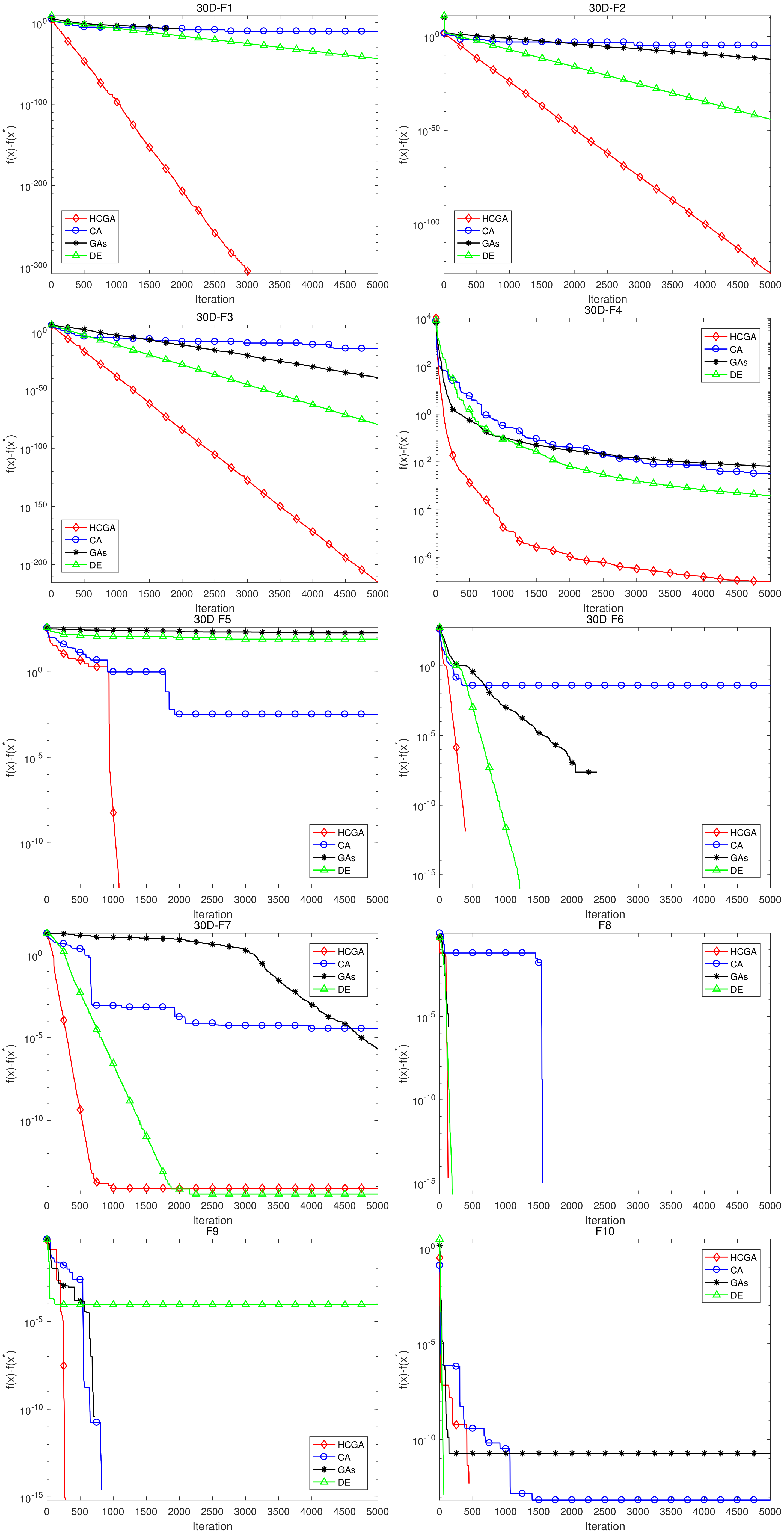
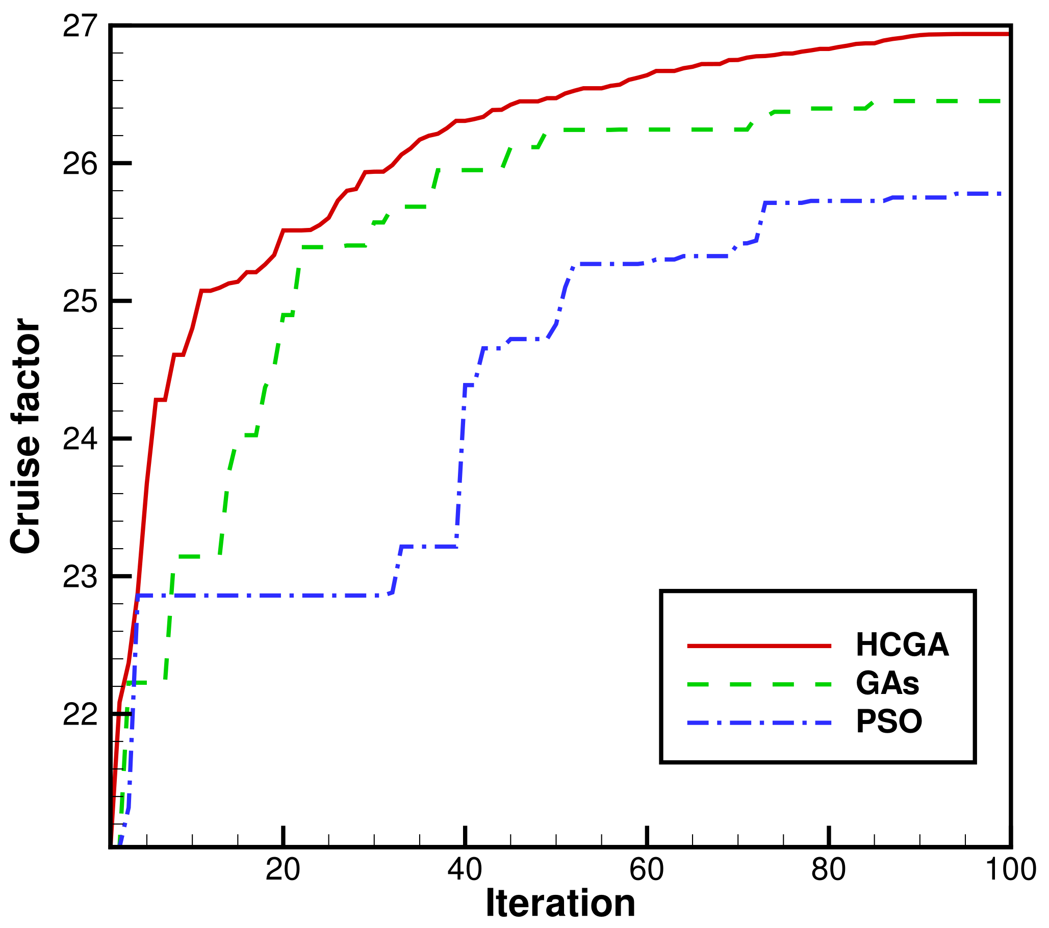
In this paper, an efficient hybrid evolutionary optimization method coupling CA with GAs (HCGA) was proposed to improve the efficiency of the optimization procedure for the aerodynamic shape of an aircraft. HCGA aims to improve the ability to solve complex problems and increase the efficiency of optimization. To improve the robustness of the algorithm, HCGA uses GAs as an evolutionary model of the population space. HCGA constructs the belief space using three kinds of knowledge: situational knowledge, normative knowledge and historical knowledge. Meanwhile, the knowledge-guided t-mutation operator was developed to dynamically adjust the mutation step and balance the exploitation and exploration ability of the algorithm. The optimization performance of HCGA was demonstrated on many benchmark functions for which the global optima are known a priori. The optimization results obtained with the benchmark functions show that HCGA provides a better global convergence, a better convergence speed and a better optimization accuracy compared to CA and GAs. In particular, HCGA shows the potential for solving large-scale design variable optimization problems.

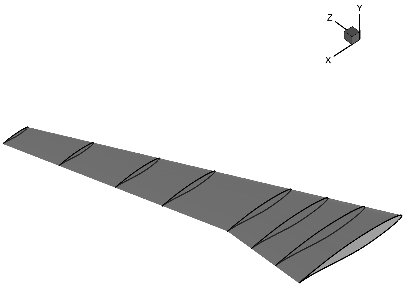
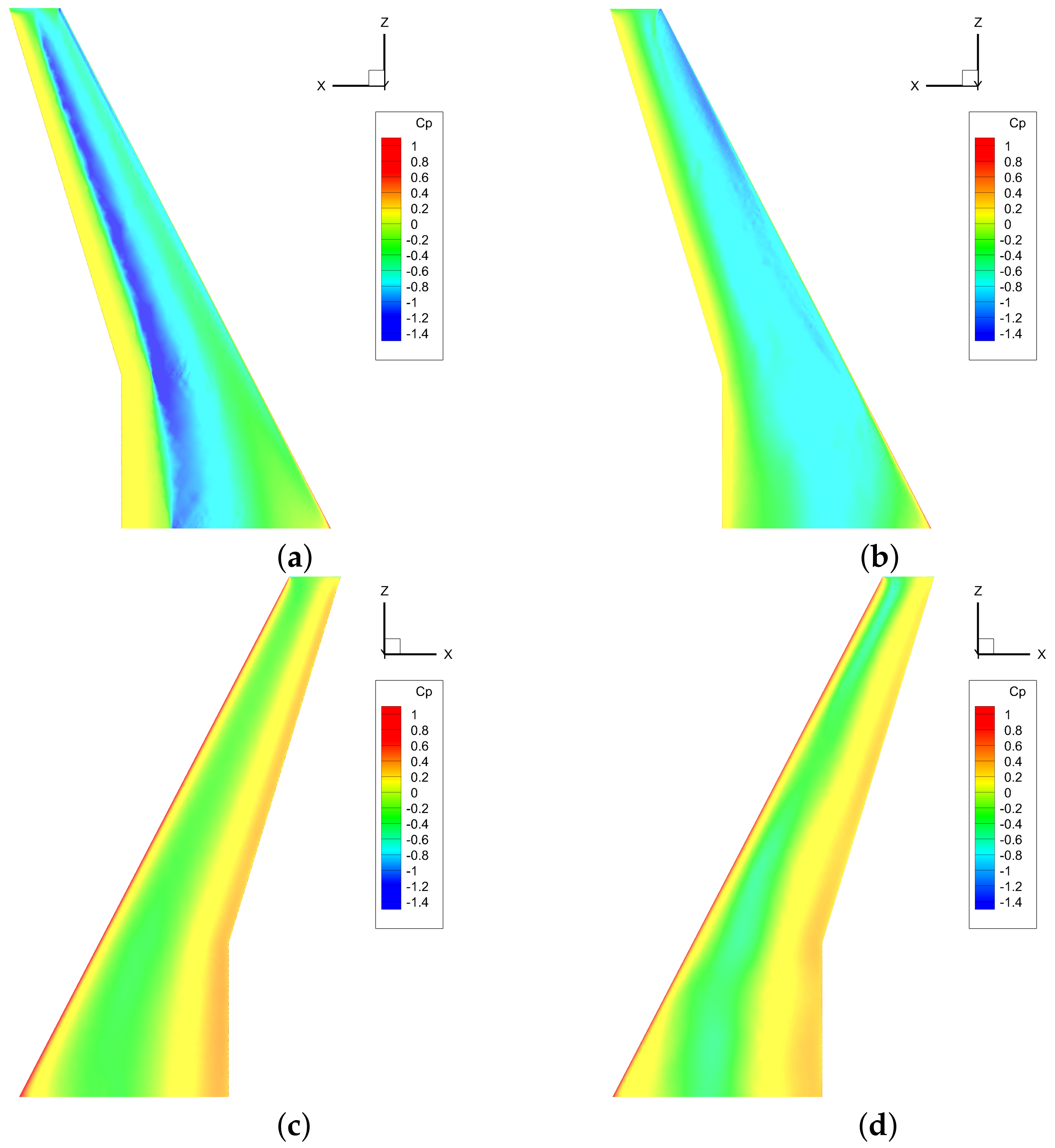
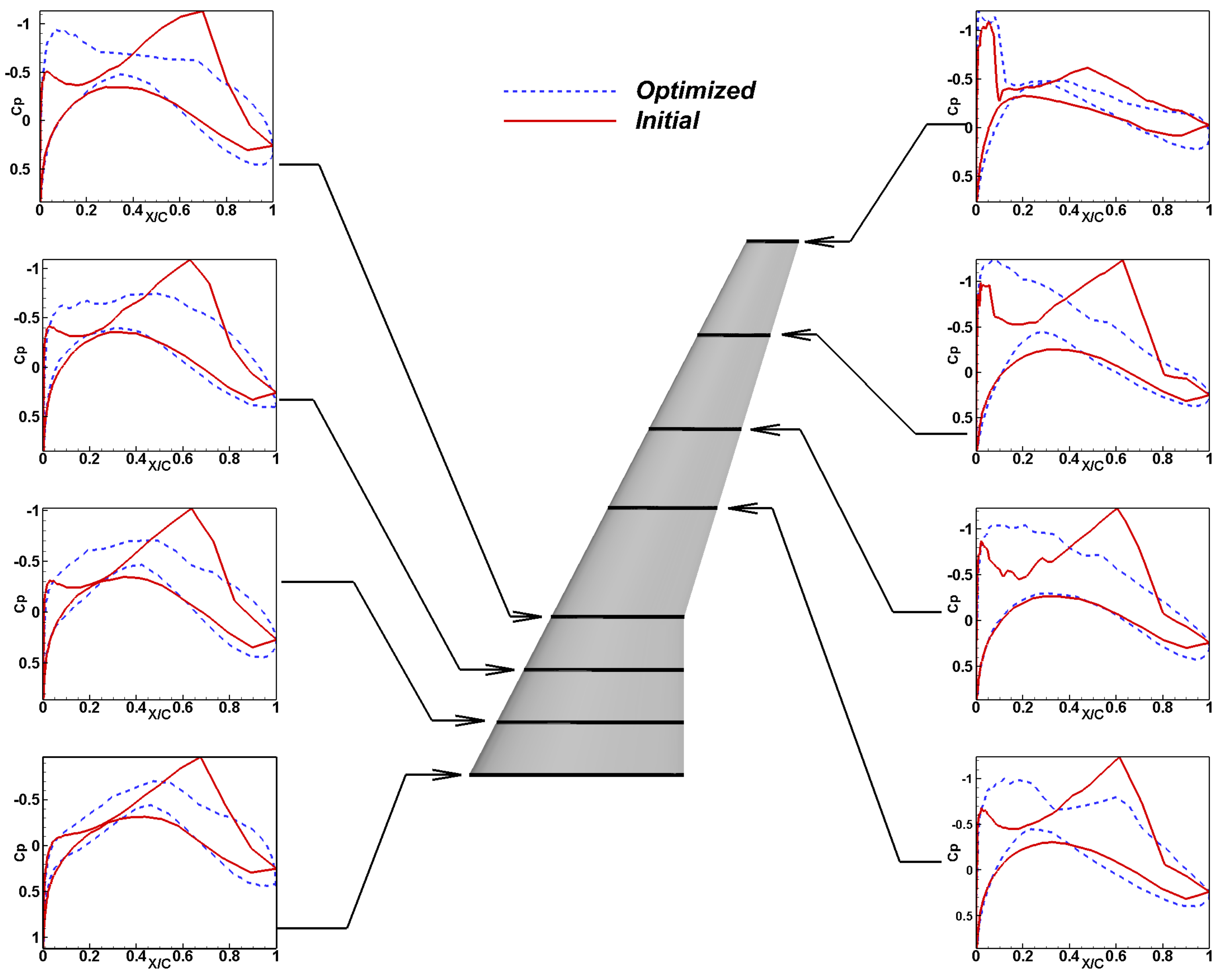
By combining HCGA with a CFD solver, an efficient decision-maker design tool for aerodynamic shape design optimization was developed to find the best aerodynamic shape to satisfy the design requirements. For the three-dimensional wing design problem, the proposed HCGA optimizer successfully reduced the wing drag computerized design, thus significantly improving the wing cruise factor. Compared with the baseline wing, the drag coefficient was reduced by 18.88%, which resulted in a 23.21% improvement in the cruise factor. This proves the capability and potential of HCGA for solving complex engineering design problems in aerodynamics. As a practical engineering application of the super-heuristic algorithm, the potential and value of such algorithms for engineering applications are further validated.

However, this study is only preliminary and further testing is needed to evaluate the performance of HCGA in complex engineering optimization. In addition, the practical application of HCGA only considered single-objective optimization. Multi-objective optimization problems should thus be the next step for investigation in future research.

References

1. Tian, X.; Li, J. A novel improved fruit fly optimization algorithm for aerodynamic shape design optimization. Knowl.-Based Syst. 2019, 179, 77–91. [Google Scholar] [CrossRef]
2. Tang, Z.; Hu, X.; Périaux, J. Multi-level hybridized optimization methods coupling local search deterministic and global search evolutionary algorithms. Arch. Comput. Methods Eng. 2020, 27, 939–975. [Google Scholar] [CrossRef]
3. Jameson, A. Aerodynamic design via control theory. J. Sci. Comput. 1988, 3, 233–260. [Google Scholar] [CrossRef] [Green Version]
4. Lee, B.J.; Kim, C. Aerodynamic redesign using discrete adjoint approach on overset mesh system. J. Aircr. 2008, 45, 1643–1653. [Google Scholar] [CrossRef]
5. Luo, J.Q.; Xiong, J.T.; Liu, F. Aerodynamic design optimization by using a continuous adjoint method. Sci. China Phys. Mech. Astron. 2014, 57, 1363–1375. [Google Scholar] [CrossRef]
6. Antunes, A.P.; Azevedo, J.L.F. Studies in aerodynamic optimization based on genetic algorithms. J. Aircr. 2014, 51, 1002–1012. [Google Scholar] [CrossRef]
7. Mi, B.; Cheng, S.; Luo, Y.; Fan, H. A new many-objective aerodynamic optimization method for symmetrical elliptic airfoils by PSO and direct-manipulation-based parametric mesh deformation. Aerosp. Sci. Technol. 2022, 120, 107296. [Google Scholar] [CrossRef]
8. Bashir, M.; Longtin-Martel, S.; Botez, R.M.; Wong, T. Aerodynamic Design Optimization of a Morphing Leading Edge and Trailing Edge Airfoil-Application on the UAS-S45. Appl. Sci. 2021, 11, 1664. [Google Scholar] [CrossRef]
9. Zijing, L.I.U.; Xuejun, L.I.U.; Xinye, C.A.I. A new hybrid aerodynamic optimization framework based on differential evolution and invasive weed optimization. Chin. J. Aeronaut. 2018, 31, 1437–1448. [Google Scholar]
10. Duan, Y.; Cai, J.; Li, Y. Gappy proper orthogonal decomposition-based two-step optimization for airfoil design. AIAA J. 2012, 50, 968–971. [Google Scholar] [CrossRef]
11. Sugisaka, M.; Fan, X. Adaptive genetic algorithm with a cooperative mode. In Proceedings of the 2001 IEEE International Symposium on Industrial Electronics Proceedings (Cat. No. 01TH8570), Pusan, Korea, 12–16 June 2001; IEEE: Piscataway, NJ, USA, 2001; Volume 3, pp. 1941–1945. [Google Scholar]
12. Srinivas, M.; Patnaik, L.M. Adaptive probabilities of crossover and mutation in genetic algorithms. IEEE Trans. Syst. Man, Cybern. 1994, 24, 656–667. [Google Scholar] [CrossRef] [Green Version]
13. Herrera, F.; Lozano, M. Adaptive genetic operators based on coevolution with fuzzy behaviors. IEEE Trans. Evol. Comput. 2001, 5, 149–165. [Google Scholar] [CrossRef]
14. Dong, H.; Li, T.; Ding, R.; Sun, J. A novel hybrid genetic algorithm with granular information for feature selection and optimization. Appl. Soft Comput. 2018, 65, 33–46. [Google Scholar] [CrossRef]
15. Li, X.; Gao, L.; Pan, Q.; Wan, L. An effective hybrid genetic algorithm and variable neighborhood search for integrated process planning and scheduling in a packaging machine workshop. IEEE Trans. Syst. Man Cybern. Syst. 2018, 49, 1933–1945. [Google Scholar] [CrossRef]
16. Reynolds, R.G. An introduction to cultural algorithms. In Proceedings of the Third Annual Conference on Evolutionary Pro–Gramming, San Diego, CA, USA, 24–26 February 1994; World Scientific: River Edge, NJ, USA, 1994; pp. 131–139. [Google Scholar]
17. dos Santos Coelho, L.; Souza, R.C.T.; Mariani, V.C. Improved differential evolution approach based on cultural algorithm and diversity measure applied to solve economic load dispatch problems. Math. Comput. Simul. 2009, 79, 3136–3147. [Google Scholar] [CrossRef]
18. Sun, Y.; Zhang, L.; Gu, X. A hybrid co-evolutionary cultural algorithm based on particle swarm optimization for solving global optimization problems. Neurocomputing 2012, 98, 76–89. [Google Scholar] [CrossRef]
19. Gao, F.; Liu, H.; Zhao, Q.; Cui, J. Hybrid model of genetic algorithms and cultural algorithms for optimization problem. In Proceedings of the Asia-Pacific Conference on Simulated Evolution and Learning, Hefei, China, 15–18 October 2006; Springer: Berlin/Heidelberg, Germany, 2006; pp. 441–448. [Google Scholar]
20. Azad, P.; Navimipour, N.J. An energy-aware task scheduling in the cloud computing using a hybrid cultural and ant colony optimization algorithm. Int. J. Cloud Appl. Comput. (IJCAC) 2017, 7, 20–40. [Google Scholar] [CrossRef]
21. Wang, X.; Hao, W.; Li, Q. An adaptive cultural algorithm with improved quantum-behaved particle swarm optimization for sonar image detection. Sci. Rep. 2017, 7, 1–16. [Google Scholar]
22. Awad, N.H.; Ali, M.Z.; Suganthan, P.N.; Reynolds, R.G. CADE: A hybridization of cultural algorithm and differential evolution for numerical optimization. Inf. Sci. 2017, 378, 215–241. [Google Scholar] [CrossRef]
23. Deng, L.; Yang, P.; Liu, W. Artificial Immune Network Clustering Based on a Cultural Algorithm. EURASIP J. Wirel. Commun. Netw. 2020, 2020, 168. [Google Scholar] [CrossRef]
24. Kulkarni, V.R.; Desai, V. Sensor Localization in Wireless Sensor Networks Using Cultural Algorithm. Int. J. Swarm Intell. Res. (IJSIR) 2020, 11, 106–122. [Google Scholar] [CrossRef]
25. Abdolrazzagh-Nezhad, M.; Radgohar, H.; Salimian, S.N. Enhanced cultural algorithm to solve multi-objective attribute reduction based on rough set theory. Math. Comput. Simul. 2020, 170, 332–350. [Google Scholar] [CrossRef]
26. Awad, N.H.; Ali, M.Z.; Duwairi, R.M. Cultural algorithm with improved local search for optimization problems. In Proceedings of the 2013 IEEE Congress on Evolutionary Computation, Cancun, Mexico, 20–23 June 2013; IEEE: Piscataway, NJ, USA, 2013; pp. 284–291. [Google Scholar]
27. Xue, H. Adaptive Cultural Algorithm-Based Cuckoo Search for Time-Dependent Vehicle Routing Problem with Stochastic Customers Using Adaptive Fractional Kalman Speed Prediction. Math. Probl. Eng. 2020, 2020, 7258780. [Google Scholar] [CrossRef]
28. Reynolds, R.G. The cultural algorithm: Culture on the edge of chaos. In Culture on the Edge of Chaos; Springer: Cham, Switzerland, 2018; pp. 1–11. [Google Scholar]
29. Ali, M.Z.; Awad, N.H.; Suganthan, P.N.; Reynolds, R.G. A modified cultural algorithm with a balanced performance for the differential evolution frameworks. Knowl.-Based Syst. 2016, 111, 73–86. [Google Scholar] [CrossRef]
30. Chung, C.J. Knowledge-Based Approaches to Self-Adaptation in Cultural Algorithms; Wayne State University: Detroit, MI, USA, 1997. [Google Scholar]
31. Saleem, S.M. Knowledge-Based Solution to Dynamic Optimization Problems Using Cultural Algorithms; Wayne State University: Detroit, MI, USA, 2001. [Google Scholar]
32. Becerra, R.L.; Coello, C.A.C. Culturizing differential evolution for constrained optimization. In Proceedings of the Fifth Mexican International Conference in Computer Science, ENC 2004, Colima, Mexico, 24 September 2004; IEEE: Piscataway, NJ, USA, 2004; pp. 304–311. [Google Scholar]
33. Opara, K.R.; Arabas, J. Differential Evolution: A survey of theoretical analyses. Swarm Evol. Comput. 2019, 44, 546–558. [Google Scholar] [CrossRef]
34. Samareh, J. Aerodynamic shape optimization based on free-form deformation. In Proceedings of the 10th AIAA/ISSMO Multidisciplinary Analysis and Optimization Conference, Albany, NY, USA, 30 August–1 September 2004; p. 4630. [Google Scholar]
35. Andersson, F.; Kvernes, B. Bezier and B-Spline Technology; Umea University Sweden: Umea, Sweden, 2003. [Google Scholar]
36. Straathof, M.H.; van Tooren, M.J.L. Extension to the class-shape-transformation method based on B-splines. AIAA J. 2011, 49, 780–790. [Google Scholar] [CrossRef]
37. Kennedy, J.; Eberhart, R. Particle swarm optimization. In Proceedings of the ICNN’95-International Conference on Neural Networks, Perth, WA, USA, 27 November–1 December 1995; IEEE: Piscataway, NJ, USA, 1995; Volume 4, pp. 1942–1948. [Google Scholar]
Figure 1. Framework of the cultural algorithm (CA).
Applsci 12 03482 g001
Figure 2. Pseudo-code of cultural algorithm.
Applsci 12 03482 g002
Figure 3. Framework of HCGA.
Applsci 12 03482 g003
Figure 4. Structure of historical knowledge.
Applsci 12 03482 g004
Figure 5. Probability density functions of the Cauchy and Gaussian distributions.
Applsci 12 03482 g005
Figure 6. Convergence curves of the test functions.
Applsci 12 03482 g006
Figure 7. Distribution of the wing sections.
Applsci 12 03482 g007
Figure 8. (a) Pressure coefficient contours on the wing upper surface of the initial wing; (b) Pressure coefficient contours on the wing upper surface of the optimized wing; (c) Pressure coefficient contours on the wing lower surface of the initial wing; (d) Pressure coefficient contours on the wing lower surface of the optimized wing.
Applsci 12 03482 g008
Figure 9. Comparison of surface pressure coefficient distributions for initial and optimized wings.
Applsci 12 03482 g009
Figure 10. Comparison of initial and optimized wing-section shapes.
Applsci 12 03482 g010
Figure 11. Convergence curves of cruising factor.
Applsci 12 03482 g011