Abstract
The diagnosis and surgical resection using Magnetic Resonance (MR) images in brain tumors is a challenging task to minimize the neurological defects after surgery owing to the non-linear nature of the size, shape, and textural variation. Radiologists, clinical experts, and brain surgeons examine brain MRI scans using the available methods, which are tedious, error-prone, time-consuming, and still exhibit positional accuracy up to 2–3 mm, which is very high in the case of brain cells. In this context, we propose an automated Ultra-Light Brain Tumor Detection (UL-BTD) system based on a novel Ultra-Light Deep Learning Architecture (UL-DLA) for deep features, integrated with highly distinctive textural features, extracted by Gray Level Co-occurrence Matrix (GLCM). It forms a Hybrid Feature Space (HFS), which is used for tumor detection using Support Vector Machine (SVM), culminating in high prediction accuracy and optimum false negatives with limited network size to fit within the average GPU resources of a modern PC system. The objective of this study is to categorize multi-class publicly available MRI brain tumor datasets with a minimum time thus real-time tumor detection can be carried out without compromising accuracy. Our proposed framework includes a sensitivity analysis of image size, One-versus-All and One-versus-One coding schemes with stringent efforts to assess the complexity and reliability performance of the proposed system with K-fold cross-validation as a part of the evaluation protocol. The best generalization achieved using SVM has an average detection rate of 99.23% (99.18%, 98.86%, and 99.67%), and F-measure of 0.99 (0.99, 0.98, and 0.99) for (glioma, meningioma, and pituitary tumors), respectively. Our results have been found to improve the state-of-the-art (97.30%) by 2%, indicating that the system exhibits capability for translation in modern hospitals during real-time surgical brain applications. The method needs 11.69 ms with an accuracy of 99.23% compared to 15 ms achieved by the state-of-the-art to earlier to detect tumors on a test image without any dedicated hardware providing a route for a desktop application in brain surgery.
1. Introduction
The brain, working with billions of cells, is diagnosed as tumorous due to uncontrolled cell division forming an abnormal colony inside or outside its periphery. It has the world’s highest morbidity and mortality rates of cancers for adults and children [1]. Brain tumor origin cannot be marked along with its growth rate. It is broadly identified as primary or secondary tumors. The former has a rate of 70% of entire brain tumors having origin inside the brain. The most heinous of these is the primary brain tumor, which is mostly malignant. Some of the primary brain tumors, namely gliomas (80% of all malignant brain tumors, only Grade I is benign out of Grades I to IV) [2], meningioma, and pituitary, are most challenging for their early detection and treatment by physicians. Glioma, initiating in the glial cells of the brain, is the prevailing one in comparison to the other two types of tumors. Meningioma, mostly benign [3], is found inside the skull and its origin is in the membrane covering the spinal cord and the brain. Pituitary tumors are found attached to the pituitary gland, whose main function is to control the hormone levels in the body. It can be benign as well as malignant, and its imbalance may lead to vision disturbances.
Presently, Magnetic Resonance Imaging (MRI) is the most common non-invasive technique preferred by radiologists that can be used for scanning, as minor structural changes become detectable that are challenging to detect using Computed Tomography (CT) based imaging. However, tumor type identification is a tedious task with the time constraint considered during the prediction stage of artificial intelligence-based solutions. Therefore, a gap is an efficient solution to the intraoperative brain surgery, encountered in the course of surgery in a timely manner. We have addressed this problem by introducing an Intelligent Ultra-Light Deep Learning framework.
In clinical imaging, most of the existing work is concerned with the automatic separation and characterization of tumors in MRI scans. Although numerous attempts were made for brain tumor detection and resection, every solution is prone to problems compromising accuracy and other body organs-related issues such as affecting the liver, spleen, kidneys, etc. The optimization of tumor resection has been achieved by applying multimodal brain tumor imaging (intraoperative magnetic resonance imaging (iMRI), neuronavigation system, intraoperative Raman spectroscopy (iRaman), intraoperative ultrasound (iUS), and real-time optical fluorescence imaging) when the solution relates to benign and malignant tumors; it leaves radiologists in an ambiguous situation about the malignant tumor type due to insufficient details [4,5]. Another problem with using medical imaging repositories is the limited number of training instances, and the most critical and difficult problem to tackle is the class imbalance, especially in a multi-class data repository.
The manual analysis of MRI scans is time-consuming for expert radiologists as well as physicians, especially in complicated cases [6]. The complex cases usually demand radiologists to compare tumor tissues with contiguous regions, enhancing images to improve the quality of perception before tumor type categorization. This situation is impractical for large amounts of data, and the manual techniques are not reproducible. Early brain tumor detection with high prediction accuracy is the most critical diagnostic step for the patient’s health [3]. Novel ideas and approaches are highly desirable for prompt and accurate detection of tumors. In the case of artificial intelligence (AI) with its key enablers, Machine Learning (ML) and Deep Learning (DL) algorithms, feature extraction shares the key role in any computer-aided system in radiology as it turns data into useful information. As a rule of thumb, the features should have a maximum inter-class variance coexistent with a maximum intra-class correlation between the members of the same class. In recent years, numerous automated systems have been used to detect brain tumors using MRI scans. Hsieh et al. [7] classified brain tumors into various types using various methods, namely: region-of-interest (ROI) determination; feature extraction; and feature selection followed by classification. They combined local texture along with global histogram moments and estimated the effects of gliomas quantitatively using 107 images, 73 low- and 34 high-grade images (glioma). Sachdeva et al. [8] illustrated a Computer-Aided Diagnosis (CAD) system, extracting color and textural features of ROIs that were segmented, and used a Genetic Algorithm (GA) for selecting optimal features. They achieved an accuracy of 91.70% and 94.90% using Genetic Algorithm-based Support Vector Machine (GA-SVM) and GA-based Artificial Neural Network (GA-ANN), respectively. Cheng et al. [9] used a publicly available T1-weighted Contrast-Enhanced Magnetic Resonance Images (CE-MRI) dataset [10], consisting of brain MRI scans having: glioma-; meningioma-; and pituitary-tumors, and applied three features extraction methods: intensity histogram; bag-of-words (BoW) model; and Gray Level Co-occurrence Matrix (GLCM). They found that BoW outperforms low-level feature extraction methods while costing the overall complexity of the model on a higher side.
The Deep Convolutional Neural Network (DCNN) is often used for analyzing images with minimum preprocessing. LeCun [11] introduced the deep neural network ‘‘lenet’’ in text-visual applications. Through state-of-the-art studies, G. Litjens et al. [12] explained that handcrafted features might be replaced by automatic feature extraction in intensive learning approaches. Swati et al. [13] claimed 96.15% accuracy for context-based image retrieval using CNN for CE-MRI dataset with transfer learning for VGG-19 architecture. He used a strategy to fine-tune the retrieval performance and used Closed-Form Metric Learning (CFML) to compare the database and query images. Soltaninejad et al. [14] used the superpixel technique, and their method classified each superpixel. They ensured robust classification by introducing a number of novel image features extracted from each superpixel viz. intensity-based, Gabor textons, fractal analysis, and curvatures. The binary classification, based on tumor and non-tumor classes, was carried out using extremely randomized trees (ERT) classifier and SVM. Soltaninejad et al. [15] introduced a 3D supervoxel based learning system for tumor segmentation in multimodal MRI brain images. For each supervoxel, the extracted first-order intensity statistical features are fed to a random forest (RF) classifier to categorize each supervoxel into tumor core, edema, and healthy brain tissue.
Soltaninejad et al. [16] carried out automated segmentation of brain tumors in multimodal MRI images by integrating machine-learned features, using fully convolutional networks (FCN), and handcrafted features using texton based histograms. They categorized the MRI image voxels into normal tissues and tumors’ parts by using an RF classifier. Zhang et al. [17] segmented 3DMRI for brain tumors using multiple encoders and improved the feature extraction process. They introduced Categorical Dice (CD) as a loss function to reduce the volume imbalance problem by setting dissimilar weights for different regions simultaneously. Huang et al. [18] proposed a multi-task deep learning system merging a fusion unit with varying depths for brain tumor segmentation. They used a distance-transform decoder module for the volumetric network (VNet), sharpening the segmentation contours and reducing the generation of rough boundaries. Jin et al. [19] introduced a data segmentation framework for prostate MRI using preprocessed quality enhanced images, with bicubic interpolation, fed to an improved 3D V-NET (3D PBV-Net) based on 3D-convolution, resulting in an excellent segmentation relying less on manual segmentation. Similarly, Y. Liu et al. [20] presented a CNN constituted of three sub-networks (viz. improved ResNet50, feature pyramid attention, and decoder networks) for automated zonal segmentation of the prostate. In another work, Y. Liu et al. [21] designed a multiple-scale feature pyramid- and spatial- attentive Bayesian deep learning framework for zonal segmentation of the prostate with uncertainty estimation. In recent work, Guan et al. [22] introduced AGSE-VNet for segmentation of 3D-MRI (multimodal) scans and used a Squeeze and Excite (SE) unit attached to each encoder, with Attention Guide Filter (AG) mechanism for each decoder exploiting channel-correlation to enhance the useful information discarding useless details such as noise. In our work, we focused on the tumorous region, enhancing some parts of the input data in the image by using runtime data correlation with static features.
In this work, we propose a novel and Ultra-Light Deep Learning Architecture (UL-DLA), which extract deep features along with textural features predicting MRI brain tumors with the help of SVM. The notion is to introduce a light deep learning architecture with extensive fine-tuning to achieve intraoperative brain surgery support. The paper is organized as follows: Section 2: Materials and Methods; Section 3: Results and Discussion; followed by Conclusions.
2. Material and Methods
2.1. Proposed Method
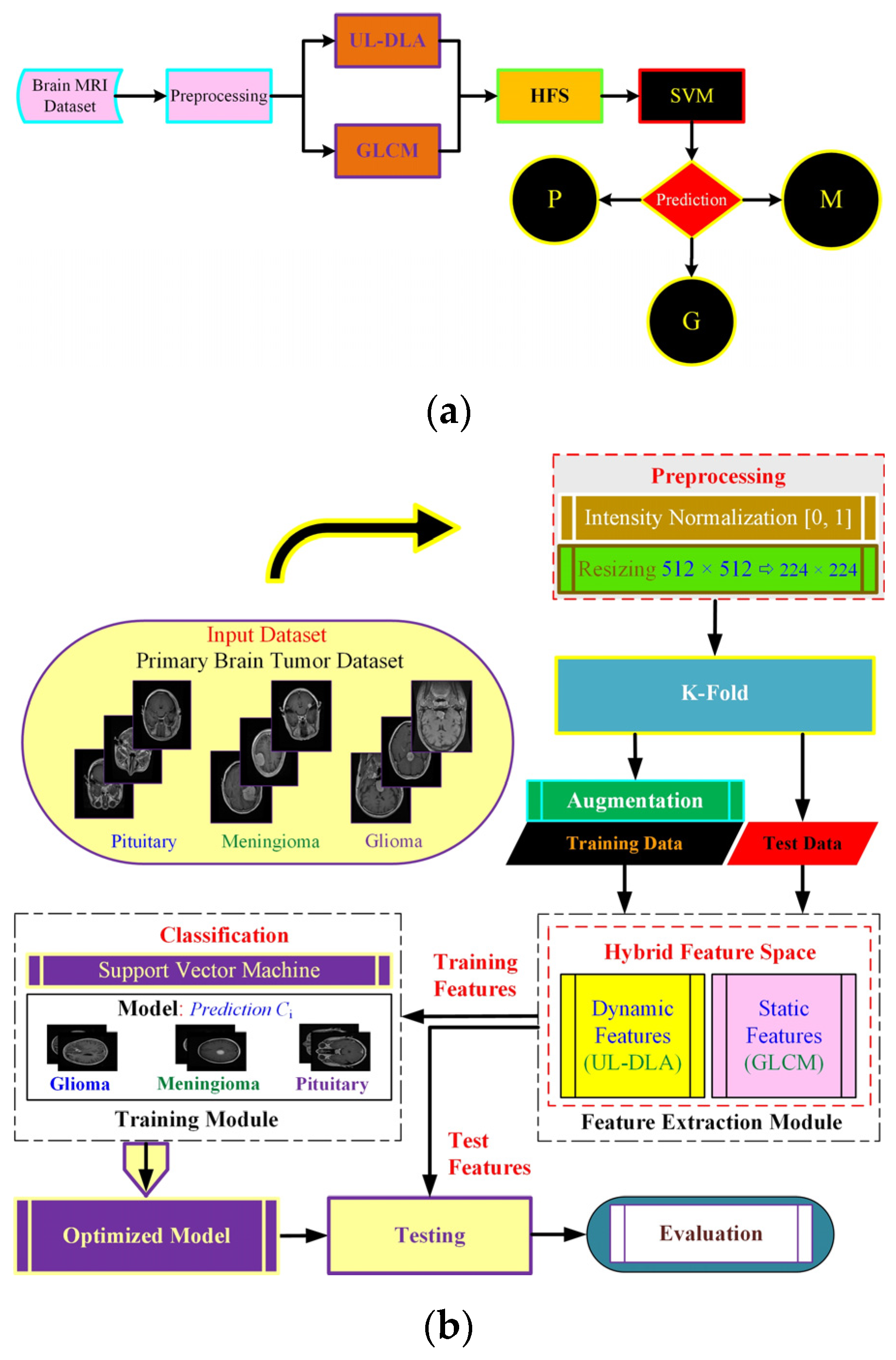
The proposed method (Figure 1) uses dynamic and static features to form a hybrid feature space (HFS). The notion was to extract dynamic features using an Ultra-Light DL architecture with accuracy enhanced by textural features viz. GLCM based static features. The resulting HFS was used to detect brain tumor type using a strong conventional SVM classifier. The feature extraction follows dataset description and preprocessing, followed by final model development.
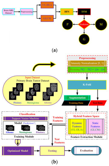
Figure 1.
The proposed Ultra-Light Brain Tumor Detection (UL-BTD) system is based on UL-DLA and textural features. Diagram (a) shows the entire workflow of the proposed technique {P: Pituitary, G: Glioma, and M: Meningioma}, whereas diagram (b) shows the phases of the proposed technique in detail.
2.2. Dataset
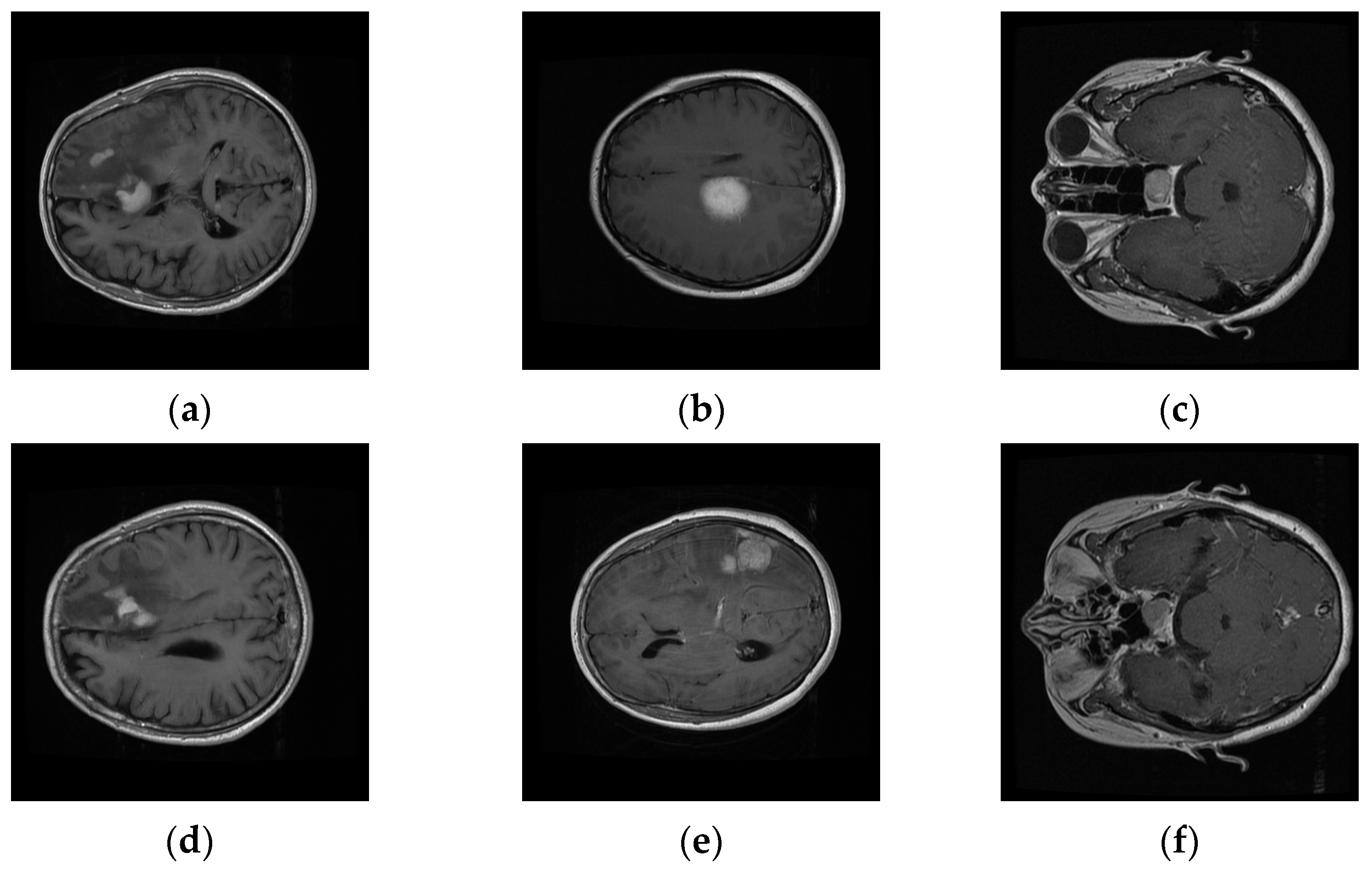
We evaluated our system on a publicly available T1-weighted CE-MRI dataset (Table 1) consisting of 2D-scanned MRI slices, as bitmap (.bmp) file types, for brain tumors: gliomas (comprising of white matter), meningioma (neighboring to gray matter, cerebrospinal fluid, and skull), and pituitary (contiguous to optic chiasma, internal carotid arteries, and sphenoidal sinus) [10]. It was donated by Nanfang Hospital, Guangzhou, China, and General Hospital, Tianjin Medical University, China, from 2005 to 2010. The dataset was imbalanced with a limited number of instances, especially for meningioma, which focused cohorts’ attention towards its challenging nature. Six rescaled sample MRI images (Figure 2) depict the variation in columns, intra-class variance, highlighting the challenging nature that is inherent in this dataset.

Table 1.
CE-MRI dataset with 3064 instances (233 patients), 512 × 512 pixels (pixel: 0.49 mm × 0.49 mm).

Figure 2.
Intra-class variation existing in three different brain tumors for transverse view: (a,d) Glioma, (b,e) Meningioma, and (c,f) Pituitary tumors’ variation in CE-MRI dataset.
2.3. Preprocessing
2.3.1. Intensity Normalization
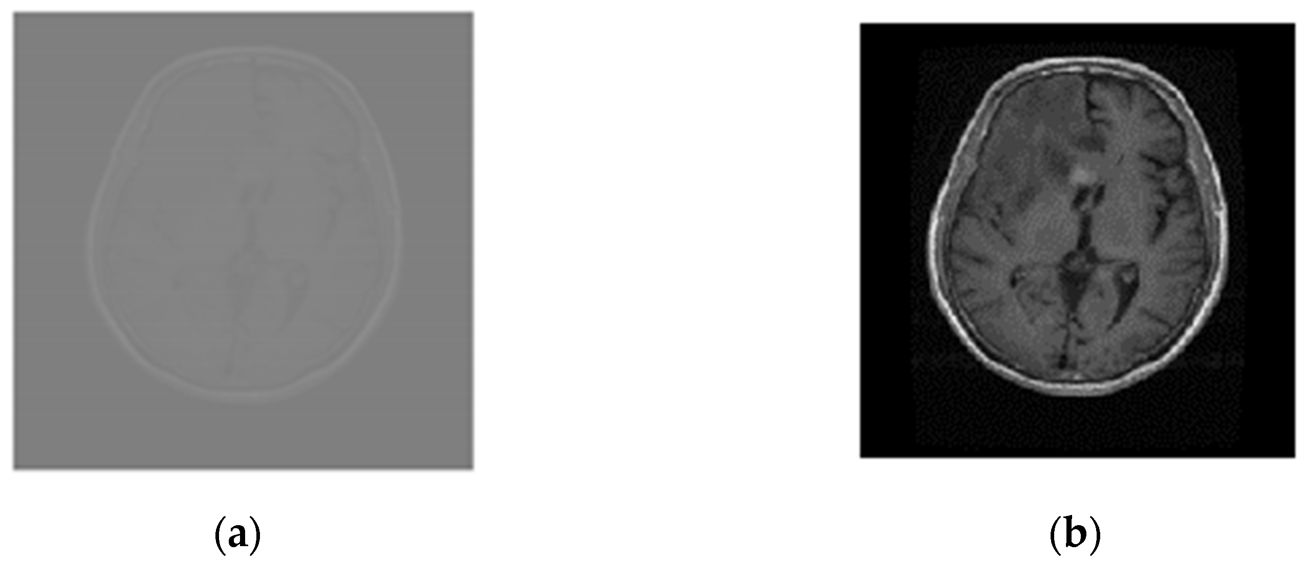
The MRI scans were linearly normalized between 0 and 1 to approach a coherent intensity range and facilitate deep learning by minimum–maximum normalization as given by: , where and represent normalized and original intensity values for the ith pixel, respectively, and represent maximum and minimum original intensity values, respectively, and used to define maximum and minimum normalized intensity values. The images, resized to 224 × 224, speed up the training process and address the out-of-memory problem especially when running on average-GPU price-based portable systems. Figure 3a,b compares images of the glioma tumor.

Figure 3.
Normalized and resized Glioma MRI scans (a) Original (512 × 512), and (b) normalized and resized (224 × 224).
2.3.2. Discrete Wavelets Based Decomposition
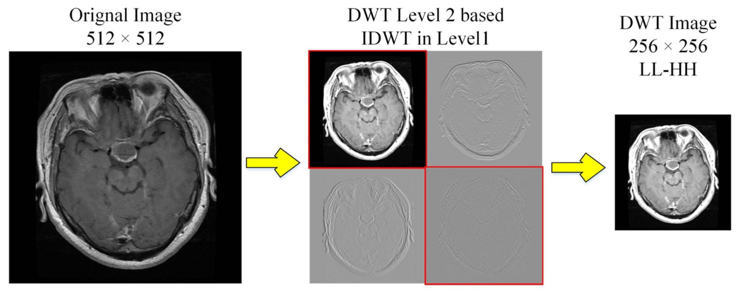
We used Discrete Wavelet Transform (DWT) for decomposition to enhance the contrast [23]. The level-2 decomposition of Haar wavelet used low (L) and high (H) pass filter banks, that generate approximation (LL) and details (LH, HL and HH) sub-band images as shown in Figure 4. We selected LL and diagonal-details (HH) of level-2 followed by inverse-DWT to level 1 before being merged to DWT image (256 × 256). This transformation follows downsampling to 224 × 224, to ensure consistency, consequently rejecting LH and HL matrices with contrast improvement.

Figure 4.
DWT decomposition of MRI scans to obtain high contrast images.
2.3.3. Augmentation
The dataset augmentation, experimented by applying geometric distortions to the MRI scans, was carried out by applying random variations to the MRI scans consisting of rotation, reflection, and shear distortions, as detailed in Table 2 [24,25]. We used 3 types of datasets for experimentation: simple CE-MRI dataset (CE-MRI); WT-based dataset (WT-CE-MRI); and augmented dataset (A-CE-MRI).
Table 2.
Geometric distortions randomly applied to the dataset.
2.4. Ultra-Light Deep Learning Architecture-Based Feature Extraction
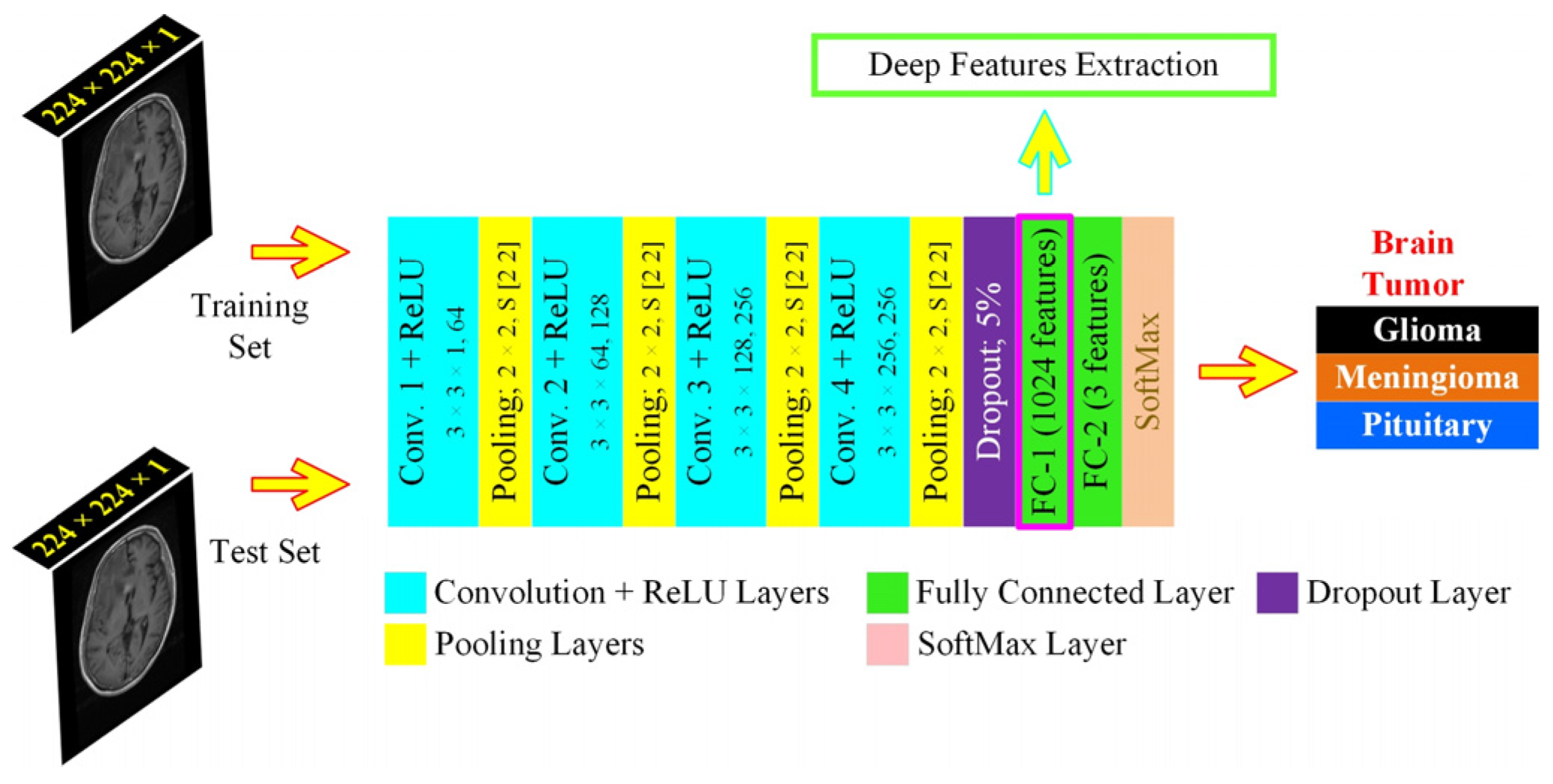
We proposed a specifically designed deep learning architecture for dynamic feature extraction, which was based on 15 layers, with each image passed through the network 20 epochs for 7 min and 10 s during the training phase, thus that the algorithmic requirements were tuned for the least resources with maximum efficiency and computational overhead, allowing its use to average GPU resources-based machines. It consisted of 4 convolution layers, as shown in Figure 5. The features from the first fully connected layer (FC1) were extracted to form the HFS. The UL-DLA based on the least number of layers with extensive fine-tuning culminated in intraoperative surgery support using the proposed framework. The specific purpose-based lighter CNN architectures were found to be performing better for tumor classification by avoiding overfitting in comparison to Inception-v3 and AlexNet [26]. For improved generalization, we used L2-regularization, along with a dropout layer, to maintain the weights and biases small. The methods and parameters that need to be initialized for UL-DLA, playing a vital role in achieving its best overall performance, were determined where some of them were empirically found, and the selected values, out of the under trial options, are illustrated in Table 3.
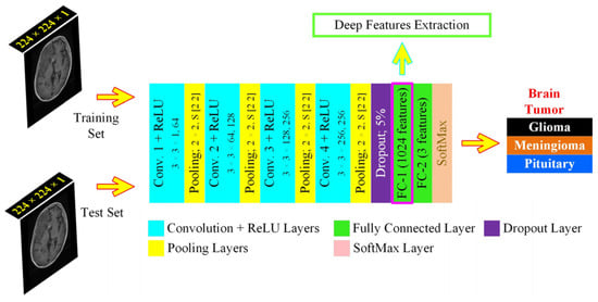
Figure 5.
The proposed Ultra-Light Deep Learning Architecture (UL-DLA) for deep features’ extraction (Conv. stride [1 1] and padding is “same”).
Table 3.
UL-DLA parameters for dynamic features extraction.
The image matrix was forwarded to the stack of convolution layers. The fully connected layer connects neurons across it and extracts features dynamically. Two fully connected layers defined in the proposed architecture were: fully connected layers 1 and 2 (FC1: 1024 neurons to capture features from the previously encoded data, and FC2: 3 neurons to capture the decision for most opted tumor category). The SoftMax layer squashes the non-normalized output of FC2 for multi-class categorization to a probability distribution for the predicted classes in the range [0, 1]. The probability for the ith class was determined from a normalized exponential function over C number of classes as given: where Oi represents ith class activation. The classification layer determines the Cross-Entropy Loss (CEL) for multi-class categorization cases and predicts the tumor type. The CEL was based on 2 sets of labels: the actual labels a(x) and the predicted labels b(x). The loss was given by: . The network training starts after preprocessing in a feed-forward manner from the input layer to the classification layer. The cost function C that is minimized with respect to weights W, being updated, during backpropagation is given by [13]: , where N is training samples count, xt represents the training sample with the actual label at and p(at|xt) is the classification probability. The minimization of C is carried out by the stochastic gradient descent method that works in the form of mini-batches of size B (16 images /batch) with 20 epochs to approximate the entire training set cost. The updated weight for iteration i + 1,, in layer L and weight updating is given by: ; , where is the mini-batch cost, is the learning rate, is the momentum controlling the influence of the previously updated weights . The conversion of 2D-data of serial convolutional layers to 1D-fully converted layers, also known as flattening, is a vulnerable step resulting in overfitting in the network.
2.5. Textural Features
In our proposed UL-BTD framework (Figure 1), another important aspect was the use of highly discriminative features extracted by grey level co-occurrence matrix (GLCM) that describes the image texture by computing repeatability of pixel-groups with specific values, and there is an existence of a definite 2-dimensional relationship in the image. We selected 13 Haralick features in our work, namely: (contrast, correlation, energy, homogeneity, mean, standard deviation, entropy, rms of image, variance, sum of image all intensities, smoothness, kurtosis, and skewness) to merge with the UL-DLA features to form HFS with a total of 1037 features.
2.6. Ultra-Light Brain Tumor Detection System
The UL-BTD system is based on HFS and potential ML algorithms such as SVM, k-NN and RF classifiers giving a convenient and reliable solution to brain tumor detection with the least resources and hardware requirements. The use of HFS on SVM for testing the UL-BTD resulted in the fastest time/image.
The optimization of SVM was achieved through linear, RBF, and polynomial kernels. We tuned the classification model using k ∈ (1, 3, 5, 7, 9) neighbors with distance metric for k-NN classifier, whereas adjusting a different set of weak learners in the range [500, 1000] trees was carried out for the RF classifier. If a point in feature space is an outlier (noise), this does not influence the decision boundaries markedly as the SVM will just ignore its effect on the model. SoftMax layer in CNN, however, will include the influence of such a point, in terms of probability-based computation, in the feature space. In other words, this results in a relatively reduced error rate using SVM with enhanced recognition capability.
2.7. Performance Measures
Reasonable efforts were carried out to tune the proposed system by standard programming tools using hardware (Laptop Dell G7, Intel® Core™ i7-8750H CPU, 2.20 GHz), 16 GB RAM, and GPU (NVIDIA GTX-1060 with 6 GB: onboard memory and 1280 CUDA cores).
Quantitative performance measures to evaluate the model include confusion matrix, true positive (TP), false negative (FN), true negative (TN), false positive (FP), positive predicted value (PPV) or precision, true positive rate (TPR) also known as recall or sensitivity, F-measure, and accuracy. F-measure is convincing in case there is a class imbalance.
3. Experimental Results and Discussion
3.1. UL-BTD Framework for Fastest Detection Time/Image Analysis
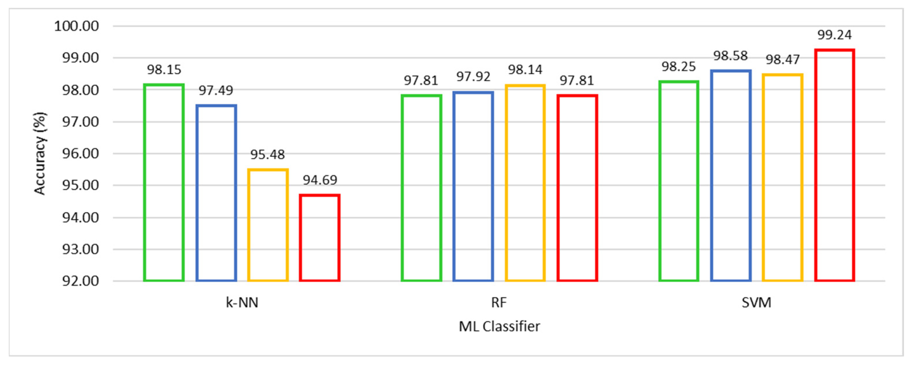
We compared competitive machine learning classifiers, viz. SVM, k-NN, and RF, using the HFS-based training, A-CE-MRI dataset, and OvA coding scheme in order to evaluate the performance of UL-BTD. The robustness and confidence of the system performance were verified by using 10-fold cross-validation for model selection on potential algorithms of choice. The results have been illustrated in Table 4, with the best results emphasized for different ML algorithms. The F-measure was computed, with other metrics, to estimate the individual and average quantitative performance, including a quantitative graphical comparison of SVM, k-NN, and RF algorithms, as shown in Figure 6. The best results have been found to be for SVM (with a polynomial of order 3: P3), with the next best found to be k-NN (with k = 1).
Table 4.
Quantitative performance comparison of UL-BTD framework for different ML algorithms using A-CE-MRI dataset with OvA coding scheme (Glioma, Meningioma and Pituitary tumors are being represented as G, M, and P respectively).
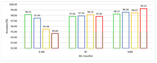
Figure 6.
Quantitative performance comparison of k-NN with k ∈ {1, 3, 5, 7}, RF with Nt ∈ {500, 550, 600, 650} and SVM with Ok ∈ {L, RBF, P2, P3} algorithms.
The well-known parameters tuned for the k-NN algorithm include k ∈ (1, 3, 5, 7, 9). Reducing k gets closer to the training data (low bias), and the model becomes dependent on the particular training samples (high variance). When k = 1 the model is being fit to the one-nearest point with the model really close to the training data. The predictability of the model with one-nearest point means the highest possibility of training on noise. The inherent intra-class variance in the dataset and random reshuffling of mini-batch data results in an excellent performance. Similarly, in the case of the RF algorithm, the number of trees (Nt) variation was thoroughly investigated, and results are shown for Nt ∈ (500, 550, 600, 650). The best tumor prediction result is achieved using (Nt = 600) trees. The RF is based on using high variance and low bias trees, resulting in a low bias and low variance forest. We need a number of trees that will improve the model’s robustness against overfitting. The excessive number of trees, accompanied by additional computational cost, leads to negligible improvement in results if any.
We experimented with SVM using kernel type (Ok) as Linear (L), Radial Basis Function (RBF), and Polynomial kernels (Po) of order (o) ∈ (2, 3, 4). Higher-order polynomials (o > 3) were not found competitive. The SVM (polynomial kernel with order 3) achieved outclass performance among the three competing algorithms. Accuracy of 99.18% was obtained to categorize glioma, 98.86% for meningioma, and 99.67% for pituitary tumors with an average accuracy of 99.24% accompanied by a minimum number (seven) of false negatives. Meningioma tumors are accompanied by a relatively low-performance index, which is attributed to the fact that it is hardest to discriminate between the two on the basis of their origin and characteristic features [25].
The visualization of three types of brain tumors using HFS, high-dimensional data, by a variant of Stochastic Neighborhood Embedding known as “t-SNE” is shown in Figure 7 for the test case as a scatterplot by assigning each feature vector a location in a non-linear manner to a lower-dimensional (two-dimension) map. It improves visualization by minimizing the central crowding tendency of the points. It may be noted that the discrimination is affected because of false events, high in Glioma and Meningioma overlapping region and our system improves discrimination for complex decision hyperplane existing between three types of tumors. From this point onward, for the rest of the experimentations, except mentioned otherwise, we integrated SVM into the UL-BTD system.
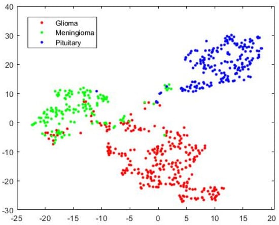
Figure 7.
The 2D scatterplot for Hybrid Feature Space (1037 features) mapped to 2 dimensions using the “t-SNE” technique.
3.2. UL-DLA and GLCM Exclusive Analysis
We have tested the usability of our model without the hybrid feature space to ascertain the effectiveness of the hybrid feature set. In order to confirm that the improvement is not just from deep features but also textural features, a SoftMax classifier experimentation was carried out using UL-DLA for 20 epochs based on deep learning features only. To avoid overfitting in the model, the dropout layer delinks 5% of the neurons for its output and input functionality (Section 2.3 and Table 3). The quantitative performance corresponding to three datasets, namely CE-MRI, WT-CE-MRI, and A-CE-MRI is illustrated in Table 5. The best overall accuracy during the test phase for the SoftMax classifier was found to be 96.882% using A-CE-MRI. The augmentation relieves the class-imbalance problem, thereby improving the results. Similarly, wavelet transform-based decomposition (WT-CE-MRI) results were improved due to high contrast in comparison to the plane dataset (CE-MRI). On the other hand, another experiment was carried out using the GLCM features only with SVM (polynomial kernel with order 3), and the quantitative results have been illustrated in Table 6. We observed that the best performance observed was attributed to the A-CE-MRI dataset with an accuracy of 86.26%. The results were indicative of the fact that textural or deep features alone were not able to achieve the required accuracy, but it was the combination of both which was able to achieve the required performance.
Table 5.
UL-DLA results using SoftMax classifier for augmented (A-CE-MRI), wavelet transform based (WT-CE-MRI), and intensity normalized (CE-MRI) images.
Table 6.
GLCM results using SVM classifier using a polynomial kernel with order 3 (test phase).
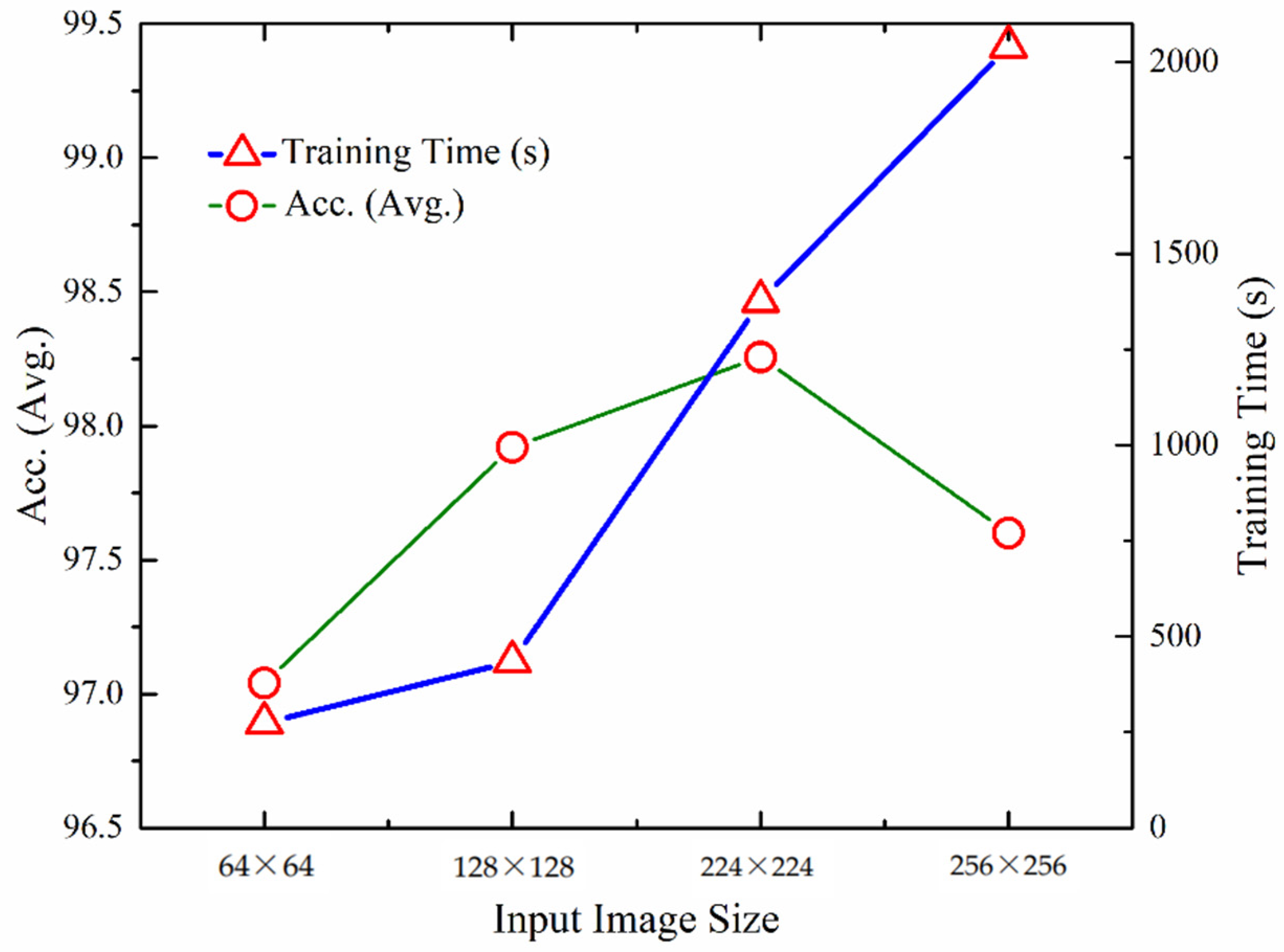
3.3. Effect of Image Size on Tumor Prediction
We carried out experimentation for measuring the quantitative performance of the UL-BTD framework for numerous input image sizes as illustrated in Table 7. The training for dynamic features was carried out using the A-CE-MRI dataset for 20 epochs, OvA as the coding scheme, and SVM with the polynomial kernel (P3). Performance increases from 64 × 64 to 224 × 224 image matrix and then drops again. The best detection rate was found to be 99.24%. In the case of smaller sizes, information was lost due to downsampling, whereas for larger image sizes (256 × 256), overfitting takes place and needs tuning by changing the dropout rate and activation function.
Table 7.
Analysis of input layer size on the proposed model using SVM in the test phase (A-CE-MRI dataset, OvA coding scheme, and polynomial kernel (P3)).
The visual representation of UL-DLA training time, excluding SVM, gives an approximation of the performance variation of the proposed methodology with image size (Figure 8). The optimum image size has been found to be 224 × 224, costing relatively more time compared to the smaller image size.
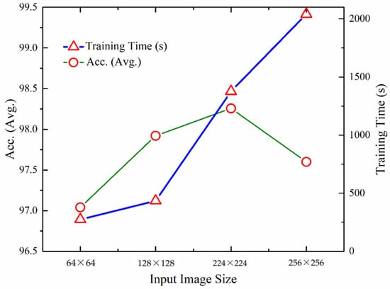
Figure 8.
Comparison of performance and training times using different input layer sizes for UL-DLA (without SVM).
3.4. Sensitivity Analysis of Coding Schemes: OvA and OvO
The multi-classification task can be performed using either of the coding schemes: One-versus-All (OvA) or One-versus-One (OvO). We experimented with both schemes without augmentation, and the results of both are given in Table 8. We found that the OvO scheme performs better than OvA with deep-layered architecture that starts from scratch. The reverse has been found true otherwise, i.e., the OvA performs better for the multi-class cases when used with pre-trained CNN architecture (transfer learning). When the proposed system starts from scratch with the OvA scheme, the results have been found slightly lacking than OvO, which is in agreement with [27].
Table 8.
Comparison of coding schemes: (OvA and OvO) for performance analysis without augmentation (G, M, and P represent glioma, meningioma, and pituitary tumors, respectively, using 224 × 224 image size).
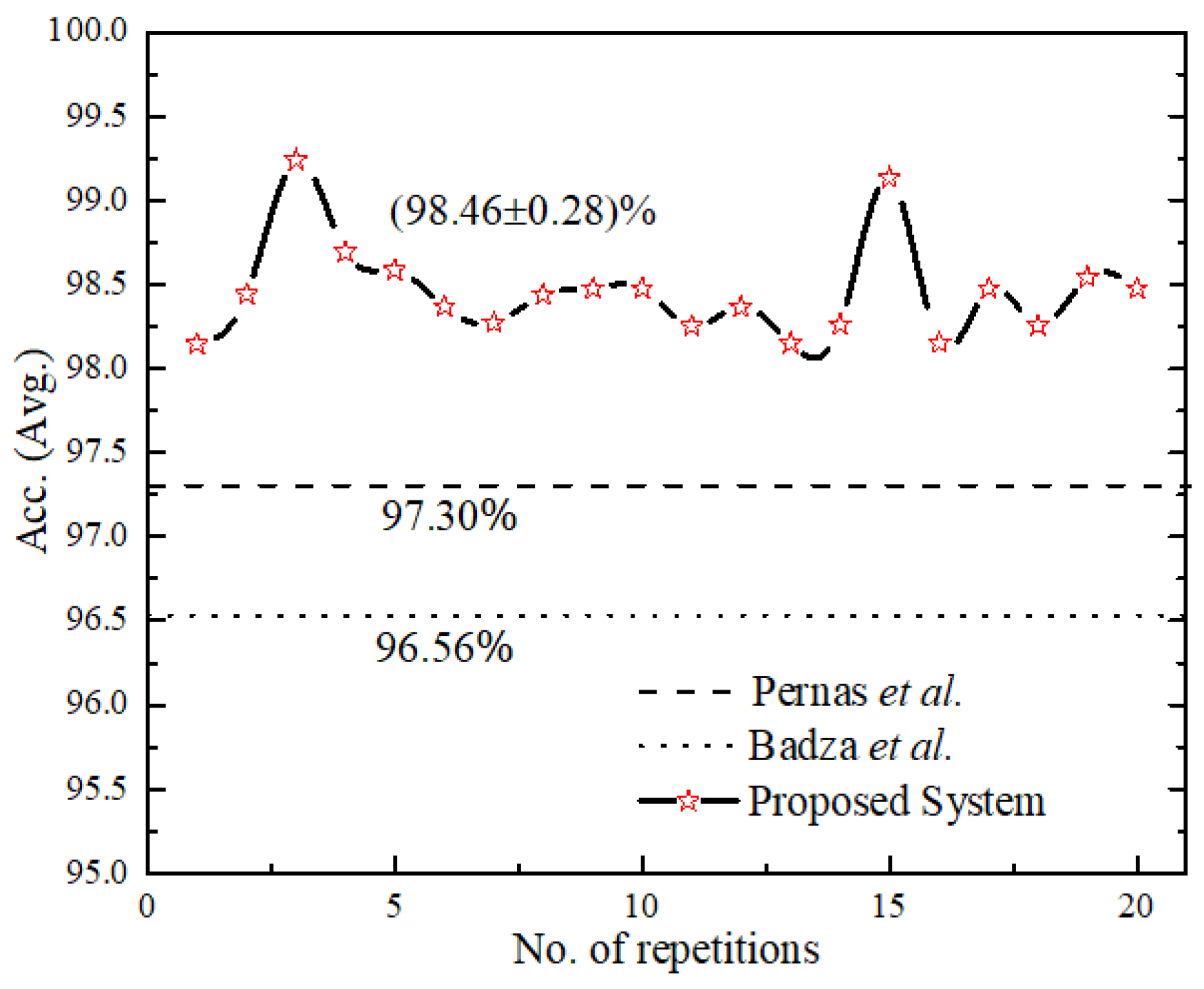
3.5. Reliability Performance and Complexity Analysis of Proposed Model
The reliability performance of the proposed system was validated for 20 consecutive runs as shown in Figure 9, with an accuracy (avg.) as (98.46 ± 0.28). We compared the proposed UL-BTD system with the two best-known, as illustrated in Table 9, for the light architecture category using the CE-MRI dataset. Our proposed system has set the new standard by 1.89 to 2.16% accuracy increase, using 18 layers (15 layers when extracting features) of deep architecture with 20 epochs. Additionally, the size of the network was limited to fit within average GPU price hardware resources available for PC category systems. The complexity of the UL-DLA was introduced as a lighter architecture with a lesser number of layers, and SVM was evaluated using Windows 10 Education with a PC machine. Two factors that have been considered for test samples constituting 20% of A-CE-MRI are shown in Table 10, namely tumor detection time per image and GPU memory usage [28]. It is obvious that SVM is a bit costlier as compared to the UL-DLA as a classifier and takes relatively more time during the test phase. The increased performance, due to generalization improvement, of a multi-class tumor classification system using SVM, is worth making a sacrifice for this minor penalty. The generalization improvement firstly is due to the use of textural features, and secondly due to the replacement of the SoftMax classifier with a sophisticated SVM-based model.
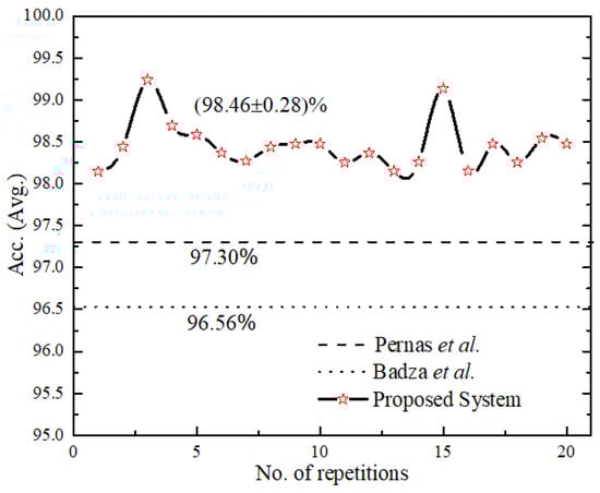
Figure 9.
Result of a consecutive run of the proposed system and for comparison with [25,32] their number of repetitions have been assumed constant.
Table 9.
Comparison of best-known results with proposed work in the light architecture category (same dataset).
Table 10.
Comparison of SVM and CNN in terms of complexity for 613 test images (20% of the dataset).
The overall reduced prediction time with no beatable accuracy per image for brain tumor classification indicates that it has the potential to act as a real-time tool during neurosurgery for accurate delineation of tumor margin using desktop computers [5,25]. The post-operative condition depends on the exposure of the tumor position; therefore, surgical support at a low cost is highly demanding especially for avoiding a second surgical attempt [4,29,30,31]. A comparison of numerous existing techniques for intraoperative brain surgery has been illustrated in Table 11. The iMRI scans along with UL-BTD Framework, can be used for tumor margin resections during real-time surgery.
Table 11.
Comparison of different intraoperative neurosurgical navigation systems with the proposed method.
3.6. Comparison with State-of-the-Art
The results of the performance comparison are summarized in Table 12 using the CE-MRI dataset. Due to the unavailability of the same split as used by other researchers, we have used (80:20)% split in addition to 10 fold (90:10)% for limited experimentation. Anaraki et al. [43] used a stochastic algorithm resulting in an accuracy of 94.20%, indicating that a more exhaustive GA-based parametric search for CNN was required. Paul et al. [44] used two CNN layers, with a uniform filter stack depth of 64 kernels in each layer and attained 91.43% accuracy. Afshar et al. [45] used extra input of tumor boundaries to improve the results by illustrating a capsule network (CapsNets) for brain tumor classification and reached an accuracy level of 89.56%. Kurup et al. [46] demonstrated the role of data preprocessing techniques to improve the CapsNets architecture for brain tumor classification with a classification accuracy of 92.60%. Gumaei et al. [47] introduced a brain tumor classification approach having three main steps: first, brain images’ transformation; second, salient features extraction; and finally, brain tumors’ classification using Regularized Extreme Learning Machine (RELM) and achieved an accuracy of 94.23%. Sultan et al. [6] proposed a CNN-based model using data augmentation and claimed an accuracy of 96.13%. Recently, Masood et al. [48] proposed a transfer learning-based customized Mask Region-Convolution Neural Network (Mask R-CNN) with a DenseNet-41 backbone architecture for classification and segmentation of brain tumors and achieved a classification accuracy of 98.34%. However, their approach was based on transfer learning, computationally intensive, and used a much larger network. Díaz-Pernas et al. [32] introduced a DCNN that included a multiscale approach for brain tumor segmentation and classification using different processing pathways with data augmentation by elastic transformation and achieved an accuracy of 97.30% using 80 epochs. The classification function counts the tumor type prediction for every pixel and considers the highest value to be the predicted tumor type.
Table 12.
Comparison with other studies for brain tumor categorization using CE-MRI dataset.
Some researchers used the same dataset using transfer learning, where the pre-trained networks were used to classify the system by changing the number of neurons in the last fully connected layer [13,49,50]. Similarly, some cohorts modified this dataset while others processed only the tumor region in an image [9,24,45,51]. In recent work, Kaplan et al. [52] achieved an accuracy of 95.56% using nLBP and αLBP features. A specifically designed solution using DCNN is simpler and faster than the pre-trained networks and do not require high-performance computing machines. VGG-16, a very deep architecture having 44 layers requires dedicated hardware for real-time performance and it is pre-trained on a huge dataset, namely ImageNet (more than one million instances) [53], using powerful computing machines for the categorization of 1000 object classes. Rehman et al. [50] augmented the brain tumor dataset and used transfer learning. He achieved the best result of 98.69% with VGG-16 pre-trained architecture using a stochastic gradient descent approach. Similarly, Kutlu and Avcı [51] achieved 98.60% accuracy by using 100 tumor images in the transverse plane for each class, with a training to test ratio of (70:30)%, using CE-MRI variant and pre-trained AlexNet. The details need to be explored for the results in case the entire dataset is used along with its generalization capability. Similarly, the methodologies requiring regions of interest, although computationally less expensive, require a dedicated panel of experts for marking the regions to work on a regular basis.
Good discriminating features exploiting diversity between the competing classes is the source of high prediction accuracy and low false negatives. These results demonstrate that the proposed UL-BTD framework outperforms state-of-the-art techniques for brain tumor classification problems. The proposed method has the highest detection rates of (99.18%, 98.86%, and 99.67%), and F-measure of (0.99, 0.97, and 0.99) for glioma, meningioma, and pituitary tumors, respectively. The reason for this lies in the preprocessed images fed to the UL-DLA for extracting dynamic features using GLCM based extremely discriminant features and then fine-tuned SVM for the brain tumor prediction system. No preprocessing of tumor region or segmentation is required rather, the rescaled images are directly used for feature extraction. The low prediction time per test image (11.69 ms) makes it suitable as a portable algorithm in developing countries on low-budget conventional PCs. Due to its low detection time, it can be used during surgical procedures for the detection of tumors [54] as the finely tuned algorithms require fewer resources for their implementation.
3.7. Contribution and Implications
We presented an intelligent Ultra-Light Deep Learning Architecture (UL-DLA) to represent learning-based features along with textural features predicting MRI brain tumor type with the help of SVM. The main focus of the framework is to support intraoperative brain surgery support by reducing the overall time to the prediction stage (Section 3.4). The Discrete Wavelet Transforms (DWT) based analysis of MRI images was carried out for contrast enhancement and downsampling of 512 × 512-sized MRI images. The challenging MRI dataset of brain tumors suffered from variations in class sizes. The class imbalance was addressed by using multi-facet augmentation. The sensitivity analysis of different classifiers for the proposed framework concluded that SVM classified better than the k-NN and RF, as well as the SoftMax classifier. The input MRI scans’ analysis established 224 × 224 sized images as the optimum choice. As far as the choice of coding schemes is concerned, out of the two multi-class coding schemes (i.e., One-Versus-One (OvO) and One-Versus-All (OvA)), OvO was found better than OvA for the proposed framework. The complexity analysis of the proposed system laid down a simple deep learning-based automated system with an overall prediction time of 11.69 ms per MRI test image compared to 15 ms per image reported by [14]. A comparison with recent techniques, using the same dataset, was presented for performance analysis, including transfer learning and fine-tuned architectures in the concluding section.
Our study has some limitations suggested as future research directions. First, the proposed framework needs the general clinical trial in the second phase for resolving the patients’ data as the second opinion in addition to the expert opinion. Second, the prediction phase or decision making in deep learning-based strategies is complex and opaque where accuracy massively depends on huge parametric space using efficient algorithms. From the XAI point of view [55,56], the proposed deep learning architecture, UL-DLA, may be analyzed with a transparent white-box for multimodal and multi-center data fusion.
4. Conclusions
In this article, we propose an Ultra-Light DL framework for features extraction forming HFS with textural features for brain tumors’ detection and resections T1-weighted CE-MRI images, based on 233 patients across the transverse, coronal, and sagittal planes with 3064 instances of three types of brain tumors: (glioma, meningioma, and pituitary). In the case of brain tumors, early detection and its automated classification is of prime importance and is still considered an open challenge to date. The tumor position, its relationship with its contiguous cells, its texture, and numerous perimeters affecting the MRI scans are some of the major highlights complicating its detection. Radiologists’ manual scanning procedure, although tedious, especially when the number of scans is enormous, is the only path to success. The salient features of this work include that it has achieved the outclass prediction accuracy with minimum false negatives for modern PC category average GPU-usage facility, with only 20 epochs to extract dynamic features using UL-DLA with a minimum number of diligently tuned layers and exploiting textural features to identify pair-wise contiguous pixel relationships causing improved discrimination identified through SVM classifier. The proposed methodology does not require any preprocessing or segmentation of the tumor region. The details related to assessing the complexity and reliability performance of the proposed system have also been carried out. To the best of our knowledge in the literature, the test results using the proposed method have the highest detection rate of 99.24% (99.18%, 98.86%, and 99.67%), and F-measure of 0.99 (0.99, 0.98, and 0.99) with 7 FNs for glioma, meningioma, and pituitary tumors, respectively. Our results have been found to be 2% better than the previously best known 97.30% in the PC desktop category system, indicating that our proposed system is highly capable of increasing diagnostic assistance to brain tumor radiologists. We strongly recommend the proposed system to act as a second opinion to the radiologists and clinical experts for this highly effective decision support system for the early diagnosis of the vulnerable population against brain tumors. The UL-BTD system has a low computational cost, with 11.69 ms detection-time per image, using even a modern PC system having average GPU resources. The proposed method has the potential use in brain tumor real-time surgery with a reduced amount of time (22.07% less) in comparison to the state-of-the-art earlier to detect a tumor without any dedicated hardware providing a route for a desktop application in brain surgery.
Author Contributions
Conceptualized the study, analyzed data, and wrote the paper, revised and edited, S.A.Q.; conceptualized the study, analyzed data, and wrote the paper, revised and edited, S.E.A.R.; analyzed data, revised, edited and supervised, L.H.; edited the paper, M.K.N.; edited the paper, A.A.M.; analyzed the data, A.u.R.; analyzed the data and edited the paper, F.N.A.-W.; edited the paper, A.M.H. All authors have read and agreed to the published version of the manuscript.
Funding
The authors extend their appreciation to the Deanship of Scientific Research at King Khalid University for funding this work under grant number (RGP 2/18/43). Princess Nourah bint Abdulrahman University Researchers Supporting Project number (PNURSP2022R151), Princess Nourah bint Abdulrahman University, Riyadh, Saudi Arabia. The authors would like to thank the Deanship of Scientific Research at Umm Al-Qura University for supporting this work by Grant Code: (22UQU4310373DSR07).
Institutional Review Board Statement
Not applicable.
Informed Consent Statement
Not applicable as the dataset is publically available.
Data Availability Statement
Previously reported data were used to support this study and are available at (https://github.com/chengjun583/brainTumorRetrieval, accessed on 1 November 2021).
Conflicts of Interest
The authors declare no conflict of interest.
References
- Siegel, R.L.; Miller, K.D.; Fedewa, S.A.; Ahnen, D.J.; Meester, R.G.; Barzi, A.; Jemal, A. Colorectal cancer statistics, 2017. CA A Cancer J. Clin. 2017, 67, 177–193. [Google Scholar] [CrossRef]
- Goodenberger, M.L.; Jenkins, R.B. Genetics of adult glioma. Cancer Genet. 2012, 205, 613–621. [Google Scholar] [CrossRef] [PubMed]
- Louis, D.N.; Perry, A.; Reifenberger, G.; Von Deimling, A.; Figarella-Branger, D.; Cavenee, W.K.; Ohgaki, H.; Wiestler, O.D.; Kleihues, P.; Ellison, D.W. The 2016 World Health Organization classification of tumors of the central nervous system: A summary. Acta Neuropathol. 2016, 131, 803–820. [Google Scholar] [CrossRef] [PubMed] [Green Version]
- Hollon, T.C.; Pandian, B.; Adapa, A.R.; Urias, E.; Save, A.V.; Khalsa, S.S.S.; Eichberg, D.G.; D’Amico, R.S.; Farooq, Z.U.; Lewis, S. Near real-time intraoperative brain tumor diagnosis using stimulated Raman histology and deep neural networks. Nat. Med. 2020, 26, 52–58. [Google Scholar] [CrossRef] [PubMed]
- DePaoli, D.; Lemoine, É.; Ember, K.; Parent, M.; Prud’homme, M.; Cantin, L.; Petrecca, K.; Leblond, F.; Côté, D.C. Rise of Raman spectroscopy in neurosurgery: A review. J. Biomed. Opt. 2020, 25, 050901. [Google Scholar] [CrossRef] [PubMed]
- Sultan, H.H.; Salem, N.M.; Al-Atabany, W. Multi-classification of brain tumor images using deep neural network. IEEE Access 2019, 7, 69215–69225. [Google Scholar] [CrossRef]
- Hsieh, K.L.-C.; Lo, C.-M.; Hsiao, C.-J. Computer-aided grading of gliomas based on local and global MRI features. Comput. Methods Programs Biomed. 2017, 139, 31–38. [Google Scholar] [CrossRef] [PubMed]
- Sachdeva, J.; Kumar, V.; Gupta, I.; Khandelwal, N.; Ahuja, C.K. A package-SFERCB-“Segmentation, feature extraction, reduction and classification analysis by both SVM and ANN for brain tumors”. Appl. Soft Comput. 2016, 47, 151–167. [Google Scholar] [CrossRef]
- Cheng, J.; Huang, W.; Cao, S.; Yang, R.; Yang, W.; Yun, Z.; Wang, Z.; Feng, Q. Enhanced performance of brain tumor classification via tumor region augmentation and partition. PLoS ONE 2015, 10, e0140381. [Google Scholar] [CrossRef] [PubMed]
- Jun, C. Brain Tumor Dataset. 2017. Available online: https://figshare.com/articles/brain_tumor_dataset/1512427 (accessed on 10 November 2021).
- LeCun, Y.; Bengio, Y.; Hinton, G. Deep learning. Nature 2015, 521, 436–444. [Google Scholar] [CrossRef] [PubMed]
- Litjens, G.; Kooi, T.; Bejnordi, B.E.; Setio, A.A.A.; Ciompi, F.; Ghafoorian, M.; Van Der Laak, J.A.; Van Ginneken, B.; Sánchez, C.I. A survey on deep learning in medical image analysis. Med. Image Anal. 2017, 42, 60–88. [Google Scholar] [CrossRef] [PubMed] [Green Version]
- Swati, Z.N.K.; Zhao, Q.; Kabir, M.; Ali, F.; Ali, Z.; Ahmed, S.; Lu, J. Content-based brain tumor retrieval for MR images using transfer learning. IEEE Access 2019, 7, 17809–17822. [Google Scholar] [CrossRef]
- Soltaninejad, M.; Yang, G.; Lambrou, T.; Allinson, N.; Jones, T.L.; Barrick, T.R.; Howe, F.A.; Ye, X. Automated brain tumour detection and segmentation using superpixel-based extremely randomized trees in FLAIR MRI. Int. J. Comput. Assist. Radiol. Surg. 2017, 12, 183–203. [Google Scholar] [CrossRef] [PubMed] [Green Version]
- Soltaninejad, M.; Yang, G.; Lambrou, T.; Allinson, N.; Jones, T.L.; Barrick, T.R.; Howe, F.A.; Ye, X. Supervised learning based multimodal MRI brain tumour segmentation using texture features from supervoxels. Comput. Methods Programs Biomed. 2018, 157, 69–84. [Google Scholar] [CrossRef] [PubMed]
- Soltaninejad, M.; Zhang, L.; Lambrou, T.; Yang, G.; Allinson, N.; Ye, X. MRI brain tumor segmentation and patient survival prediction using random forests and fully convolutional networks. In Proceedings of the International MICCAI Brainlesion Workshop, Quebec City, QC, Canada, 14 September 2017; pp. 204–215. [Google Scholar]
- Zhang, W.; Yang, G.; Huang, H.; Yang, W.; Xu, X.; Liu, Y.; Lai, X. ME-Net: Multi-encoder net framework for brain tumor segmentation. Int. J. Imaging Syst. Technol. 2021, 31, 1834–1848. [Google Scholar] [CrossRef]
- Huang, H.; Yang, G.; Zhang, W.; Xu, X.; Yang, W.; Jiang, W.; Lai, X. A deep multi-task learning framework for brain tumor segmentation. Front. Oncol. 2021, 11, 690244. [Google Scholar] [CrossRef] [PubMed]
- Jin, Y.; Yang, G.; Fang, Y.; Li, R.; Xu, X.; Liu, Y.; Lai, X. 3D PBV-Net: An automated prostate MRI data segmentation method. Comput. Biol. Med. 2021, 128, 104160. [Google Scholar] [CrossRef]
- Liu, Y.; Yang, G.; Mirak, S.A.; Hosseiny, M.; Azadikhah, A.; Zhong, X.; Reiter, R.E.; Lee, Y.; Raman, S.S.; Sung, K. Automatic prostate zonal segmentation using fully convolutional network with feature pyramid attention. IEEE Access 2019, 7, 163626–163632. [Google Scholar] [CrossRef]
- Liu, Y.; Yang, G.; Hosseiny, M.; Azadikhah, A.; Mirak, S.A.; Miao, Q.; Raman, S.S.; Sung, K. Exploring uncertainty measures in Bayesian deep attentive neural networks for prostate zonal segmentation. IEEE Access 2020, 8, 151817–151828. [Google Scholar] [CrossRef]
- Guan, X.; Yang, G.; Ye, J.; Yang, W.; Xu, X.; Jiang, W.; Lai, X. 3D AGSE-VNet: An automatic brain tumor MRI data segmentation framework. BMC Med. Imaging 2022, 22, 6. [Google Scholar] [CrossRef]
- Rajput, Y.; Rajput, V.S.; Thakur, A.; Vyas, G. Advanced image enhancement based on wavelet & histogram equalization for medical images. IOSR J. Electron. Commun. Eng. 2012, 2, 12–16. [Google Scholar]
- Sajjad, M.; Khan, S.; Muhammad, K.; Wu, W.; Ullah, A.; Baik, S.W. Multi-grade brain tumor classification using deep CNN with extensive data augmentation. J. Comput. Sci. 2019, 30, 174–182. [Google Scholar] [CrossRef]
- Badža, M.M.; Barjaktarović, M.Č. Classification of Brain Tumors from MRI Images Using a Convolutional Neural Network. Appl. Sci. 2020, 10, 1999. [Google Scholar] [CrossRef] [Green Version]
- Akbar, S.; Peikari, M.; Salama, S.; Nofech-Mozes, S.; Martel, A.L. The transition module: A method for preventing overfitting in convolutional neural networks. Comput. Methods Biomech. Biomed. Eng. Imaging Vis. 2019, 7, 260–265. [Google Scholar] [CrossRef] [PubMed]
- Pawara, P.; Okafor, E.; Groefsema, M.; He, S.; Schomaker, L.R.; Wiering, M.A. One-vs-One Classification for Deep Neural Networks. Pattern Recognit. 2020, 108, 107528. [Google Scholar] [CrossRef]
- Niu, X.-X.; Suen, C.Y. A novel hybrid CNN–SVM classifier for recognizing handwritten digits. Pattern Recognit. 2012, 45, 1318–1325. [Google Scholar] [CrossRef]
- Abraham, P.; Sarkar, R.; Brandel, M.G.; Wali, A.R.; Rennert, R.C.; Lopez Ramos, C.; Padwal, J.; Steinberg, J.A.; Santiago-Dieppa, D.R.; Cheung, V. Cost-effectiveness of intraoperative MRI for treatment of high-grade gliomas. Radiology 2019, 291, 689–697. [Google Scholar] [CrossRef] [PubMed]
- Lakomkin, N.; Hadjipanayis, C.G. The use of spectroscopy handheld tools in brain tumor surgery: Current evidence and techniques. Front. Surg. 2019, 6, 30. [Google Scholar] [CrossRef] [PubMed]
- Hu, S.; Kang, H.; Baek, Y.; El Fakhri, G.; Kuang, A.; Choi, H.S. Real-time imaging of brain tumor for image-guided surgery. Adv. Healthc. Mater. 2018, 7, 1800066. [Google Scholar] [CrossRef]
- Díaz-Pernas, F.J.; Martínez-Zarzuela, M.; Antón-Rodríguez, M.; González-Ortega, D. A Deep Learning Approach for Brain Tumor Classification and Segmentation Using a Multiscale Convolutional Neural Network. Healthcare 2021, 9, 153. [Google Scholar] [CrossRef]
- Schupper, A.J.; Rao, M.; Mohammadi, N.; Baron, R.; Lee, J.Y.; Acerbi, F.; Hadjipanayis, C.G. Fluorescence-guided surgery: A review on timing and use in brain tumor surgery. Front. Neurol. 2021, 12, 914. [Google Scholar] [CrossRef] [PubMed]
- Nguyen, Q.T.; Tsien, R.Y. Fluorescence-guided surgery with live molecular navigation—A new cutting edge. Nat. Rev. Cancer 2013, 13, 653–662. [Google Scholar] [CrossRef] [PubMed]
- Lindseth, F.; Langø, T.; Bang, J.; Nagelhus Hemes, T.A. Accuracy evaluation of a 3D ultrasound-based neuronavigation system. Comput. Aided Surg. 2002, 7, 197–222. [Google Scholar] [CrossRef] [PubMed]
- Sastry, R.; Bi, W.L.; Pieper, S.; Frisken, S.; Kapur, T.; Wells, W., III; Golby, A.J. Applications of ultrasound in the resection of brain tumors. J. Neuroimaging 2017, 27, 5–15. [Google Scholar] [CrossRef]
- Ganau, M.; Ligarotti, G.K.; Apostolopoulos, V. Real-time intraoperative ultrasound in brain surgery: Neuronavigation and use of contrast-enhanced image fusion. Quant. Imaging Med. Surg. 2019, 9, 350. [Google Scholar] [CrossRef] [PubMed]
- ul Rehman, A.; Qureshi, S.A. A review of the medical hyperspectral imaging systems and unmixing algorithms’ in biological tissues. Photodiagnosis Photodyn. Ther. 2020, 33, 102165. [Google Scholar] [CrossRef] [PubMed]
- Fabelo, H.; Ortega, S.; Lazcano, R.; Madroñal, D.; Callicó, G.M.; Juárez, E.; Salvador, R.; Bulters, D.; Bulstrode, H.; Szolna, A. An intraoperative visualization system using hyperspectral imaging to aid in brain tumor delineation. Sensors 2018, 18, 430. [Google Scholar] [CrossRef] [PubMed] [Green Version]
- Schulder, M.; Carmel, P.W. Intraoperative magnetic resonance imaging: Impact on brain tumor surgery. Cancer Control 2003, 10, 115–124. [Google Scholar] [CrossRef] [PubMed] [Green Version]
- Fan, Y.; Xia, Y.; Zhang, X.; Sun, Y.; Tang, J.; Zhang, L.; Liao, H. Optical coherence tomography for precision brain imaging, neurosurgical guidance and minimally invasive theranostics. Biosci. Trends 2018, 12, 12–23. [Google Scholar] [CrossRef] [PubMed] [Green Version]
- Kut, C.; Chaichana, K.L.; Xi, J.; Raza, S.M.; Ye, X.; McVeigh, E.R.; Rodriguez, F.J.; Quiñones-Hinojosa, A.; Li, X. Detection of human brain cancer infiltration ex vivo and in vivo using quantitative optical coherence tomography. Sci. Transl. Med. 2015, 7, ra100–ra292. [Google Scholar] [CrossRef] [PubMed] [Green Version]
- Anaraki, A.K.; Ayati, M.; Kazemi, F. Magnetic resonance imaging-based brain tumor grades classification and grading via convolutional neural networks and genetic algorithms. Biocybern. Biomed. Eng. 2019, 39, 63–74. [Google Scholar] [CrossRef]
- Paul, J.S.; Plassard, A.J.; Landman, B.A.; Fabbri, D. Deep learning for brain tumor classification. In Proceedings of the Medical Imaging 2017: Biomedical Applications in Molecular, Structural, and Functional Imaging, Orlando, FL, USA, 12–14 February 2017; p. 1013710. [Google Scholar]
- Afshar, P.; Mohammadi, A.; Plataniotis, K.N. Brain tumor type classification via capsule networks. In Proceedings of the 2018 25th IEEE International Conference on Image Processing (ICIP), Athens, Greece, 7–10 October 2018; pp. 3129–3133. [Google Scholar]
- Kurup, R.V.; Sowmya, V.; Soman, K. Effect of data pre-processing on brain tumor classification using capsulenet. In Proceedings of the International Conference on Intelligent Computing and Communication Technologies (ICICCT 2019), Istanbul, Turkey, 29–30 April 2019; pp. 110–119. [Google Scholar]
- Gumaei, A.; Hassan, M.M.; Hassan, M.R.; Alelaiwi, A.; Fortino, G. A hybrid feature extraction method with regularized extreme learning machine for brain tumor classification. IEEE Access 2019, 7, 36266–36273. [Google Scholar] [CrossRef]
- Masood, M.; Nazir, T.; Nawaz, M.; Mehmood, A.; Rashid, J.; Kwon, H.-Y.; Mahmood, T.; Hussain, A. A Novel Deep Learning Method for Recognition and Classification of Brain Tumors from MRI Images. Diagnostics 2021, 11, 744. [Google Scholar] [CrossRef] [PubMed]
- Swati, Z.N.K.; Zhao, Q.; Kabir, M.; Ali, F.; Ali, Z.; Ahmed, S.; Lu, J. Brain tumor classification for MR images using transfer learning and fine-tuning. Comput. Med. Imaging Graph. 2019, 75, 34–46. [Google Scholar] [CrossRef] [PubMed]
- Rehman, A.; Naz, S.; Razzak, M.I.; Akram, F.; Imran, M. A deep learning-based framework for automatic brain tumors classification using transfer learning. Circuits Syst. Signal Process. 2020, 39, 757–775. [Google Scholar] [CrossRef]
- Kutlu, H.; Avcı, E. A novel method for classifying liver and brain tumors using convolutional neural networks, discrete wavelet transform and long short-term memory networks. Sensors 2019, 19, 1992. [Google Scholar] [CrossRef] [PubMed] [Green Version]
- Kaplan, K.; Kaya, Y.; Kuncan, M.; Ertunç, H.M. Brain tumor classification using modified local binary patterns (LBP) feature extraction methods. Med. Hypotheses 2020, 139, 109696. [Google Scholar] [CrossRef] [PubMed]
- Russakovsky, O.; Deng, J.; Su, H.; Krause, J.; Satheesh, S.; Ma, S.; Huang, Z.; Karpathy, A.; Khosla, A.; Bernstein, M. Imagenet large scale visual recognition challenge. Int. J. Comput. Vis. 2015, 115, 211–252. [Google Scholar] [CrossRef] [Green Version]
- Moccia, S.; Foti, S.; Routray, A.; Prudente, F.; Perin, A.; Sekula, R.F.; Mattos, L.S.; Balzer, J.R.; Fellows-Mayle, W.; De Momi, E. Toward improving safety in neurosurgery with an active handheld instrument. Ann. Biomed. Eng. 2018, 46, 1450–1464. [Google Scholar] [CrossRef] [PubMed]
- Ye, Q.; Xia, J.; Yang, G. Explainable AI for COVID-19 CT classifiers: An initial comparison study. In Proceedings of the 2021 IEEE 34th International Symposium on Computer-Based Medical Systems (CBMS), Online, 7–9 June 2021; pp. 521–526. [Google Scholar]
- Yang, G.; Ye, Q.; Xia, J. Unbox the black-box for the medical explainable ai via multi-modal and multi-centre data fusion: A mini-review, two showcases and beyond. Inf. Fusion 2022, 77, 29–52. [Google Scholar] [CrossRef]

Publisher’s Note: MDPI stays neutral with regard to jurisdictional claims in published maps and institutional affiliations. |
© 2022 by the authors. Licensee MDPI, Basel, Switzerland. This article is an open access article distributed under the terms and conditions of the Creative Commons Attribution (CC BY) license (https://creativecommons.org/licenses/by/4.0/).