
Prediction of Self-Healing of Engineered Cementitious Composite Using Machine Learning Approaches


Abstract
:1. Introduction
2. Experimental Program
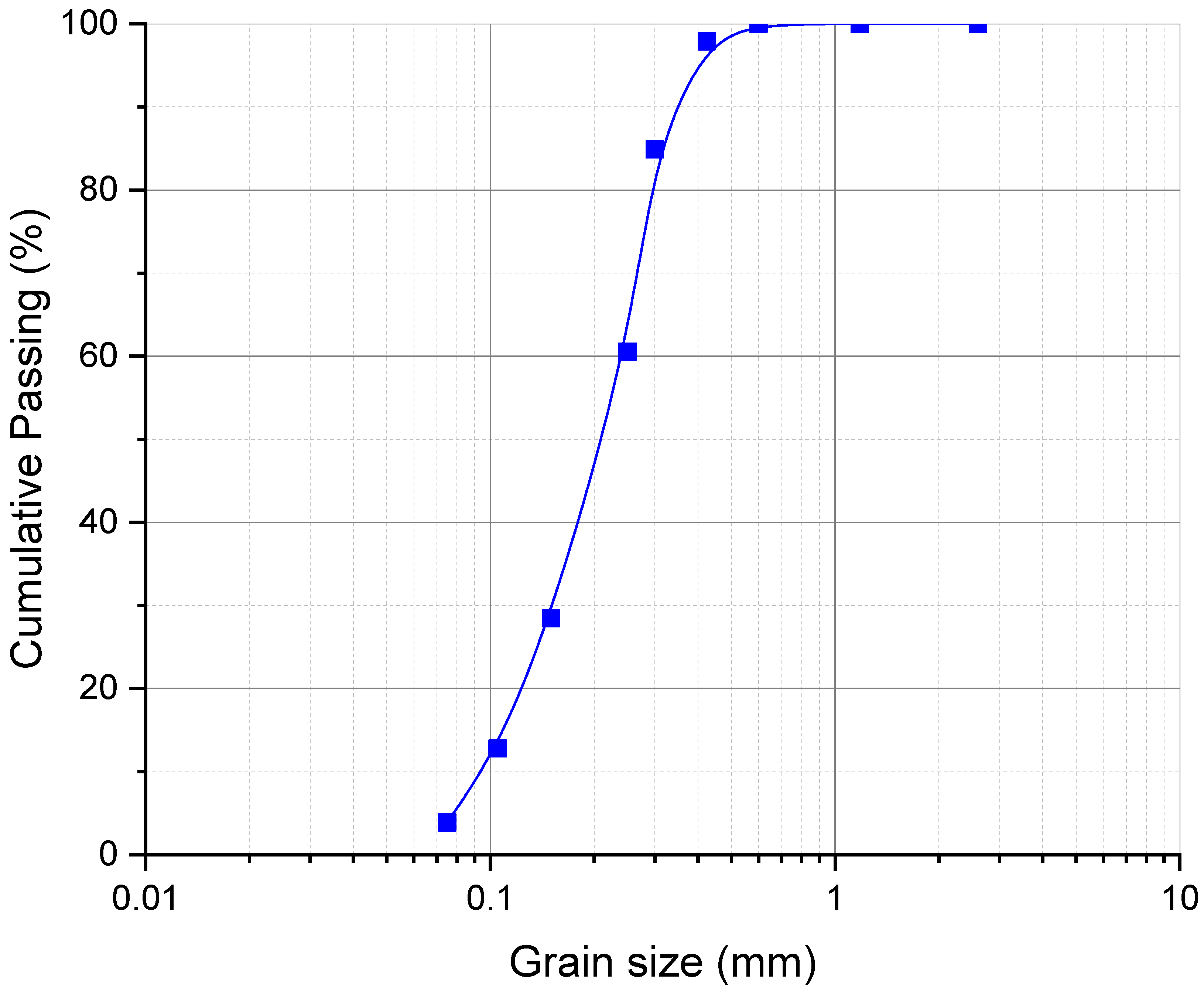
2.1. Materials and Mixture Proportion
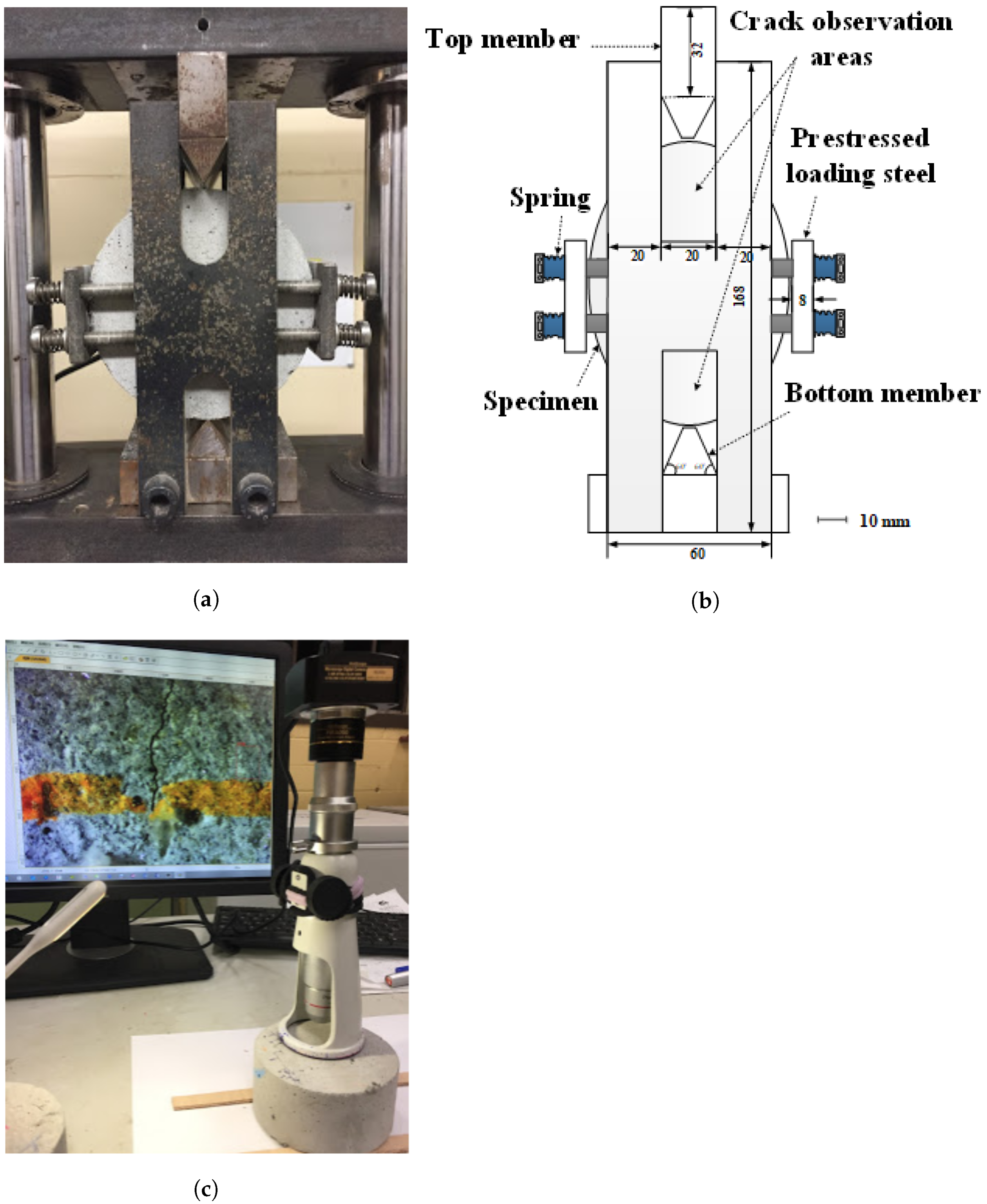
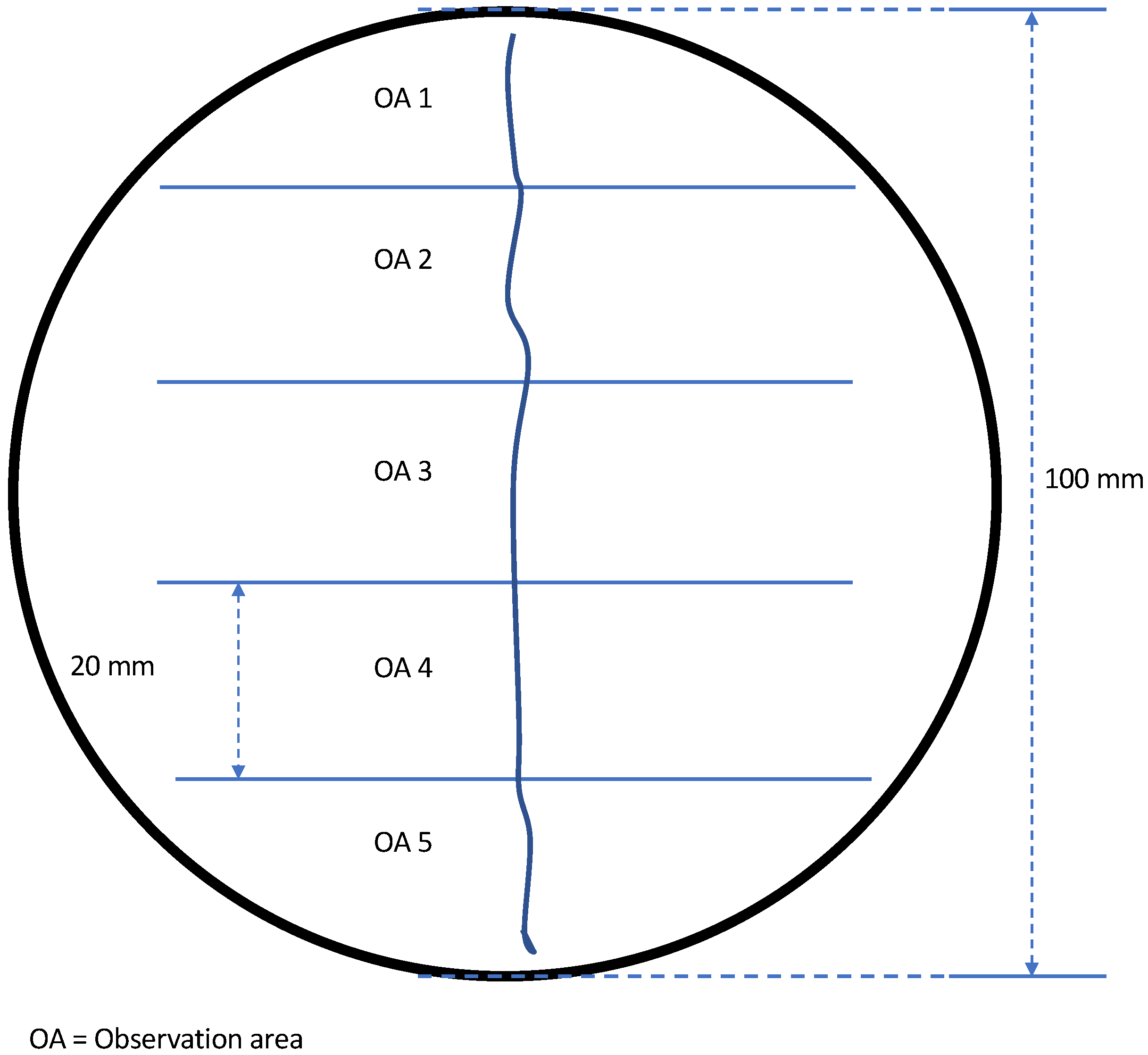
2.2. Sample Preparation and Crack Measurement
2.3. Data Collection
2.4. Preprocessing of Data
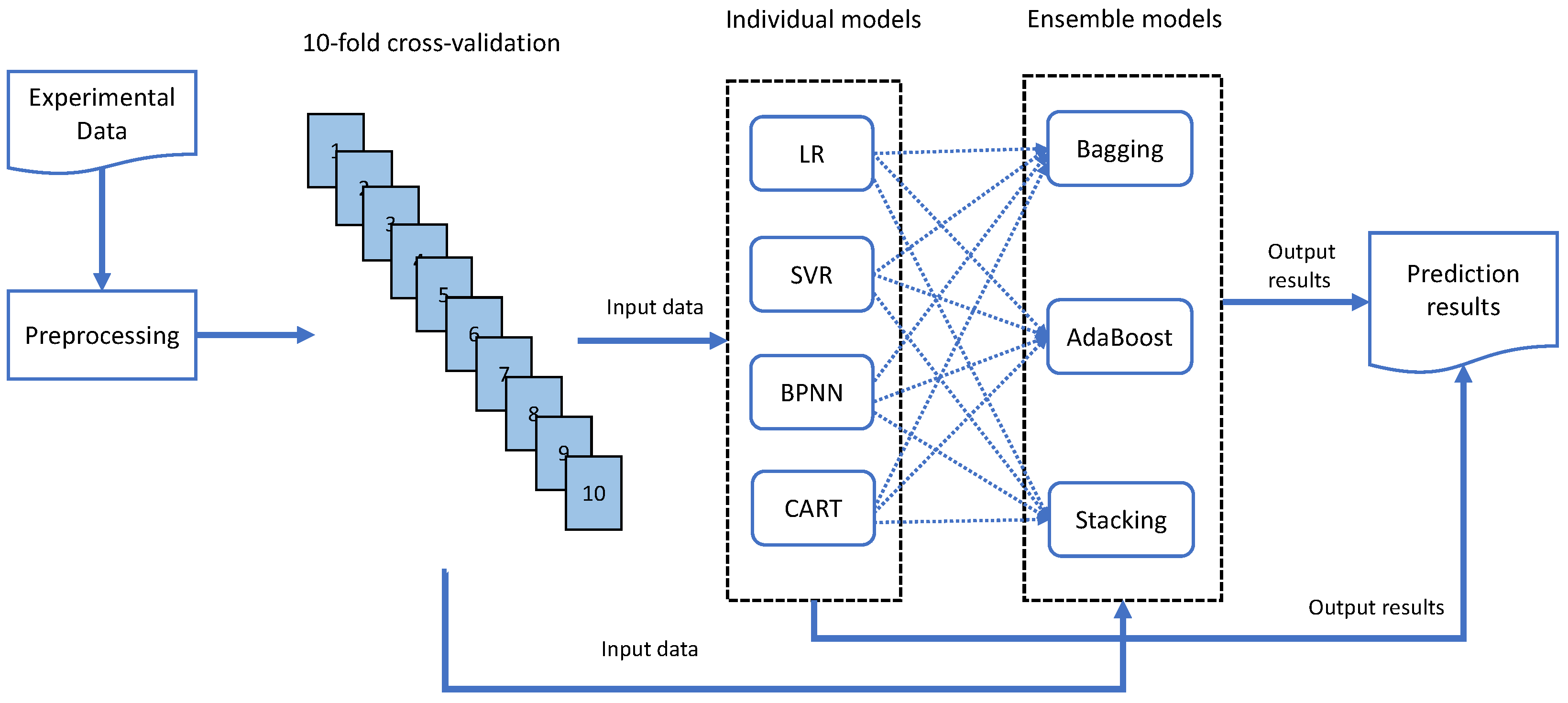
3. Proposed Machine Learning Models
3.1. Linear Regression
3.2. Support Vector Regression
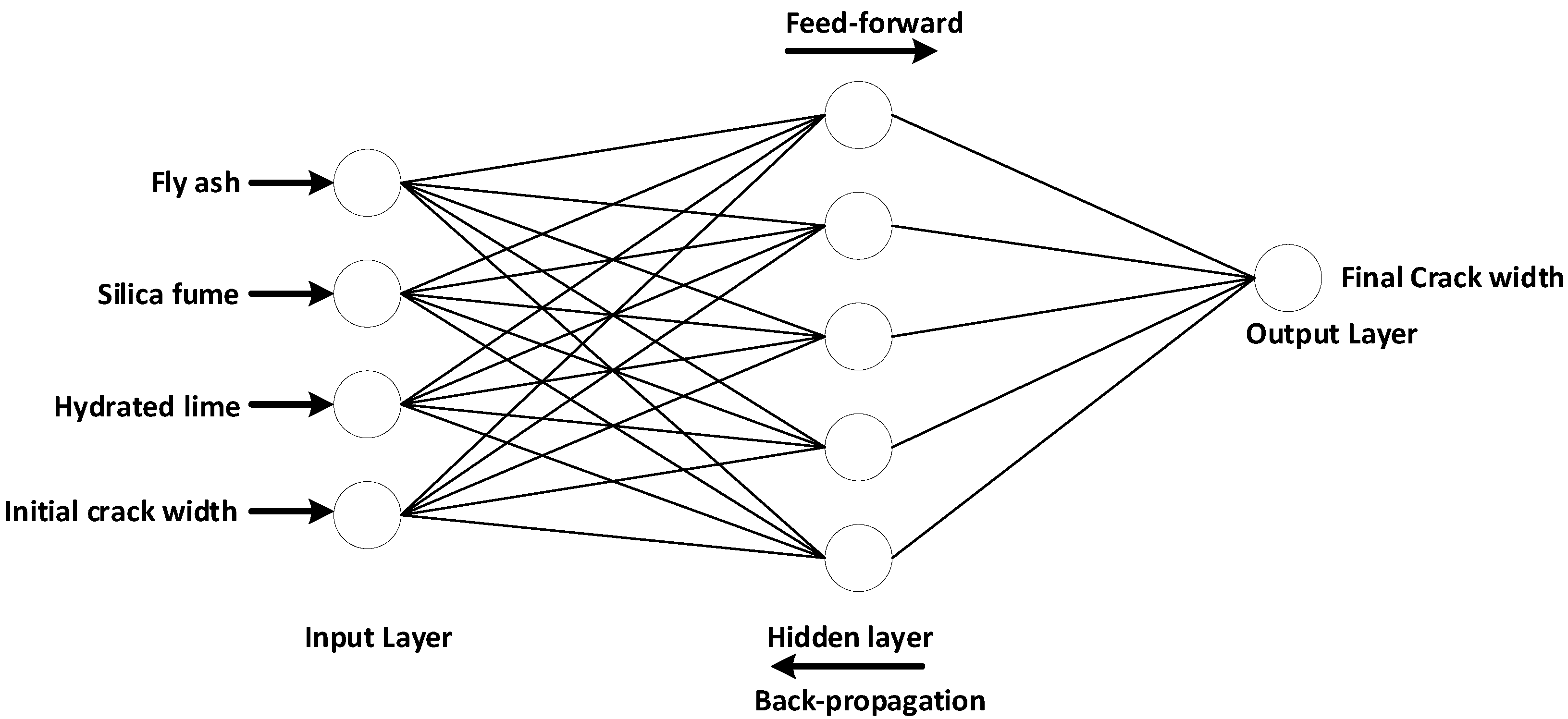
3.3. Artificial Neural Network
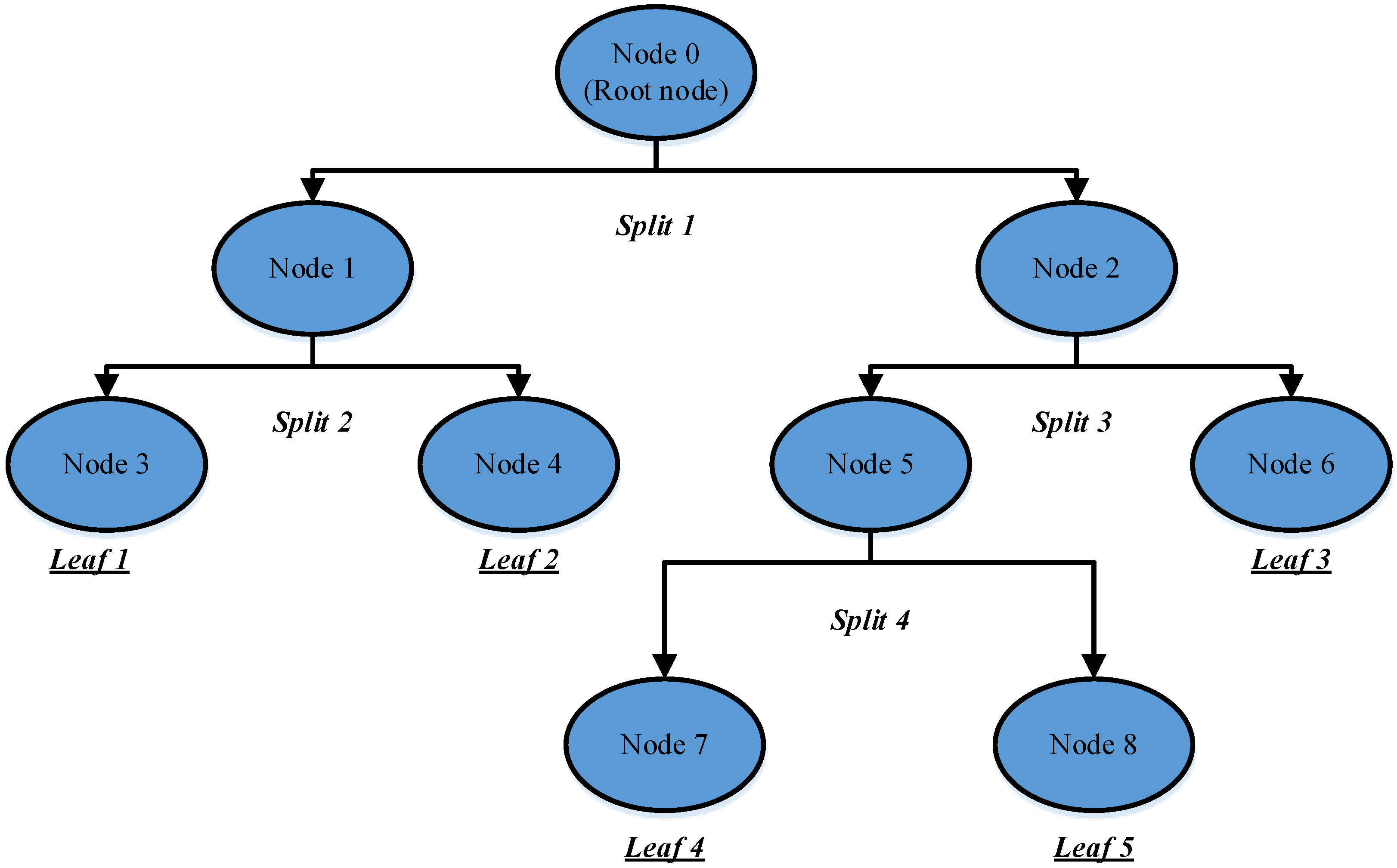
3.4. Classification and Regression Tree
3.5. Ensemble Methods
3.5.1. Bagging
3.5.2. AdaBoost
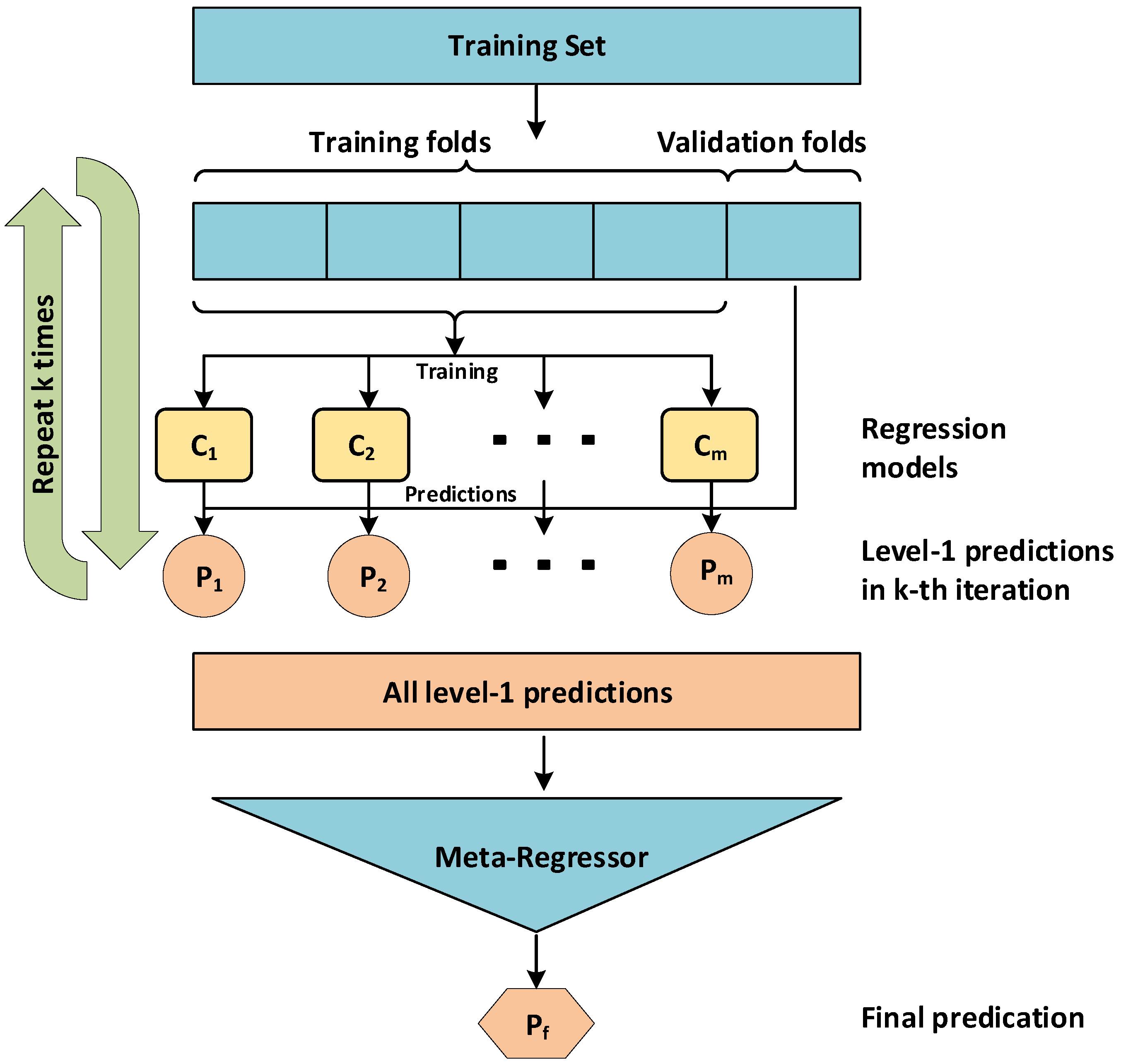
3.5.3. Stacking
4. Validation and Evaluation
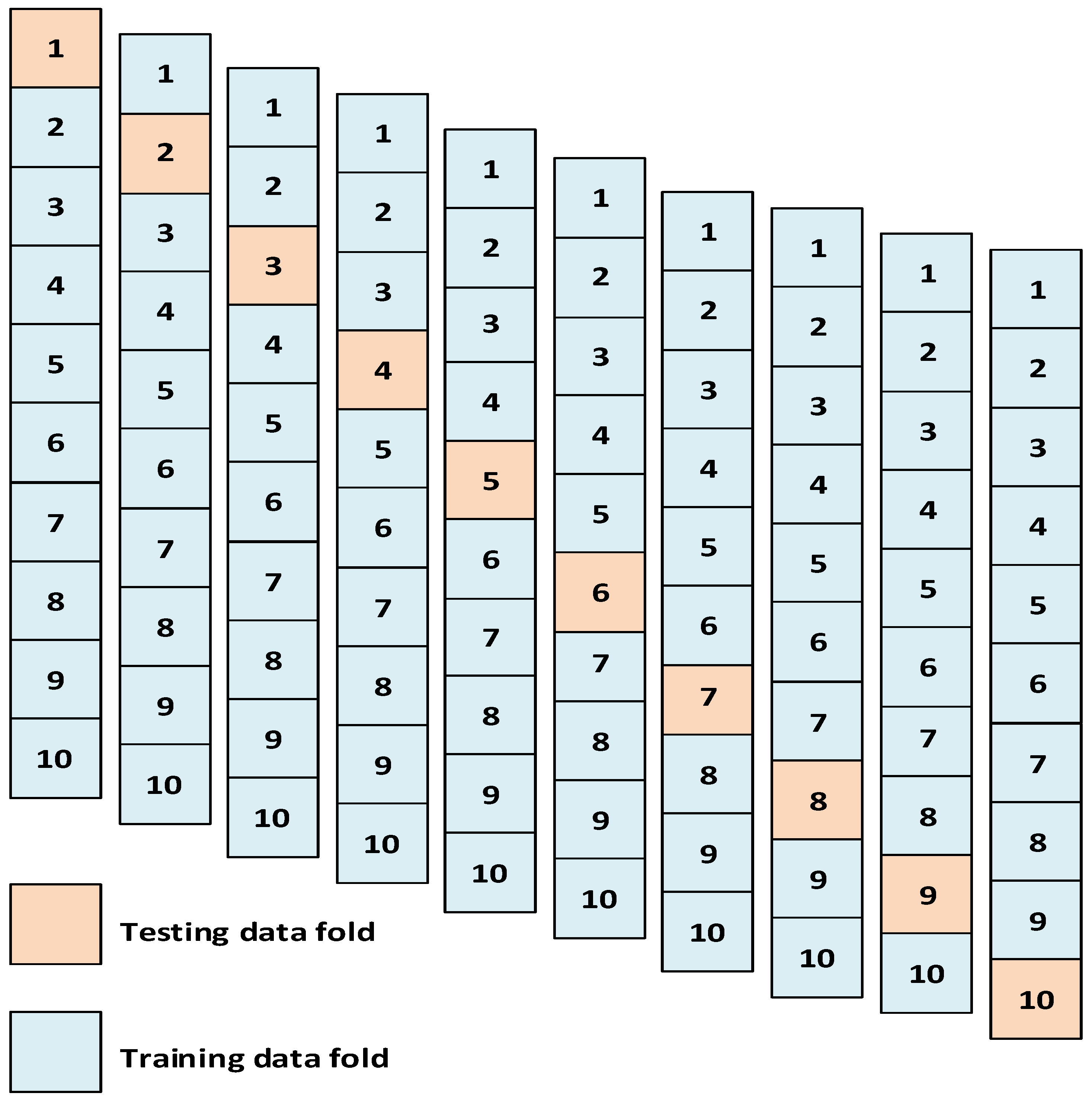
4.1. Cross-Validation Method
4.2. Performance Evaluation
- Mean absolute error (MAE).
- Root-mean-squared error (RMSE)
- Coefficient of determination ()
- Deviation ()
5. Results and Discussion
5.1. Prediction Performance of the Proposed Models
5.2. Prediction Performance Comparison
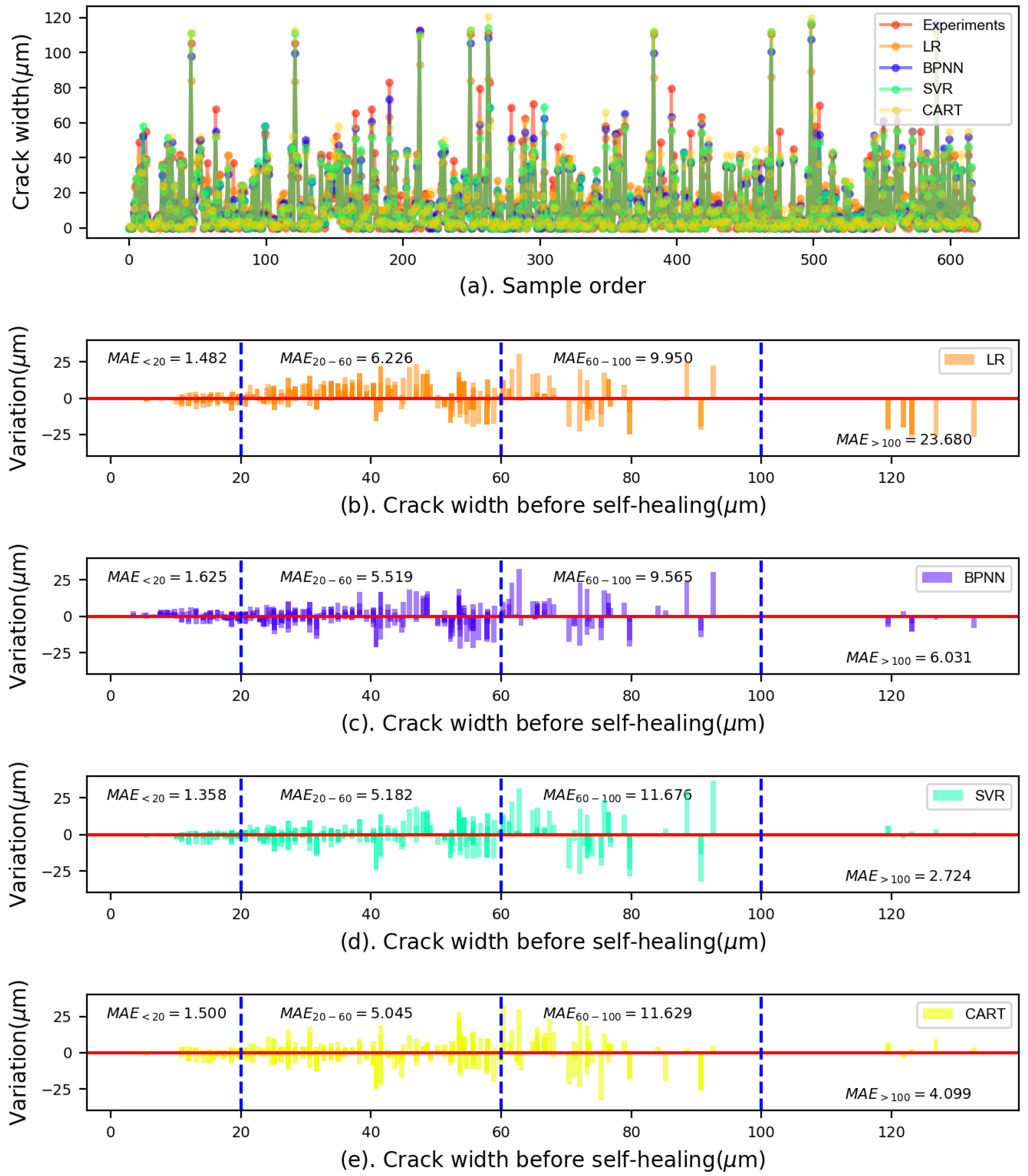
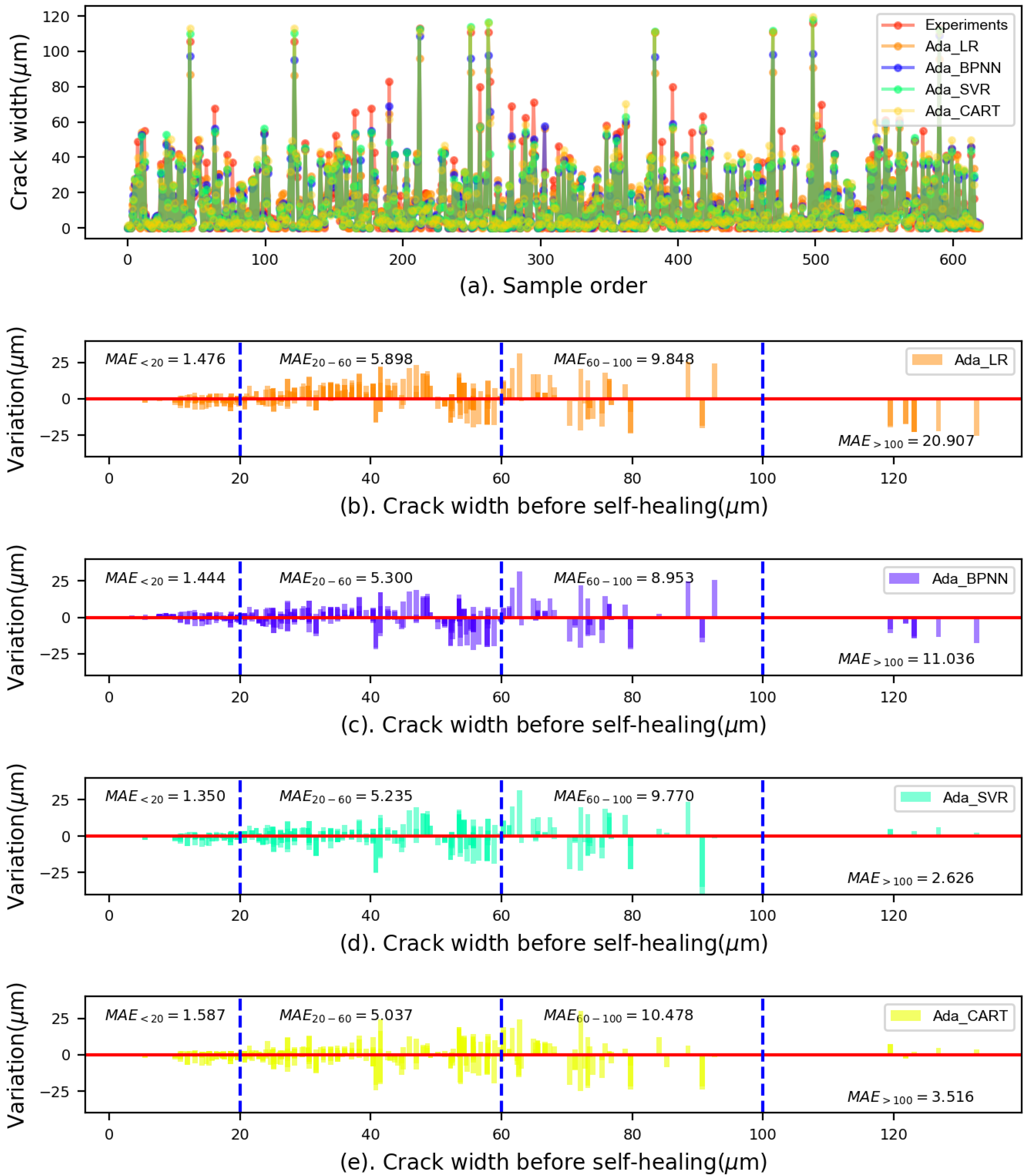
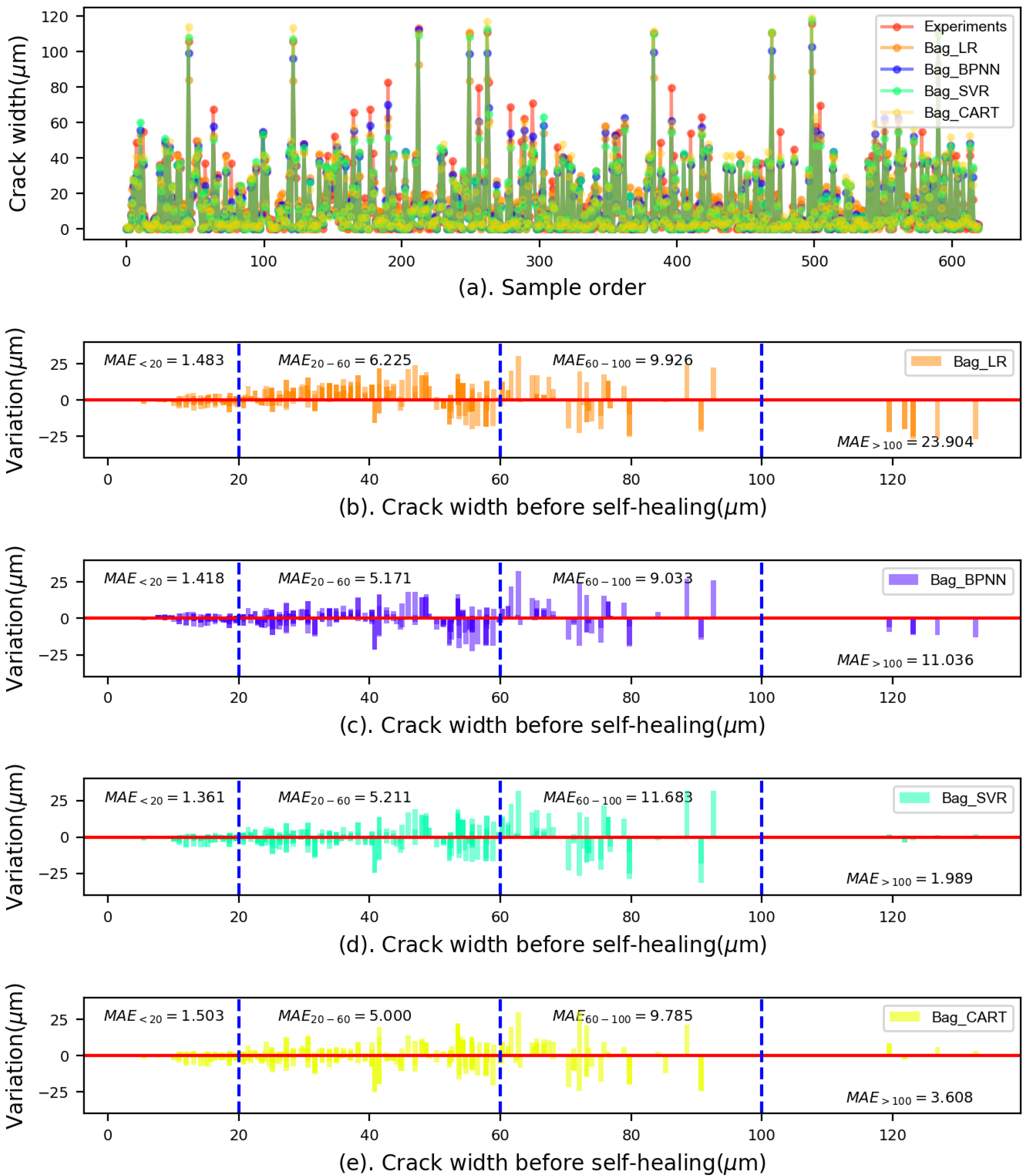
5.2.1. Comparison of the MAE
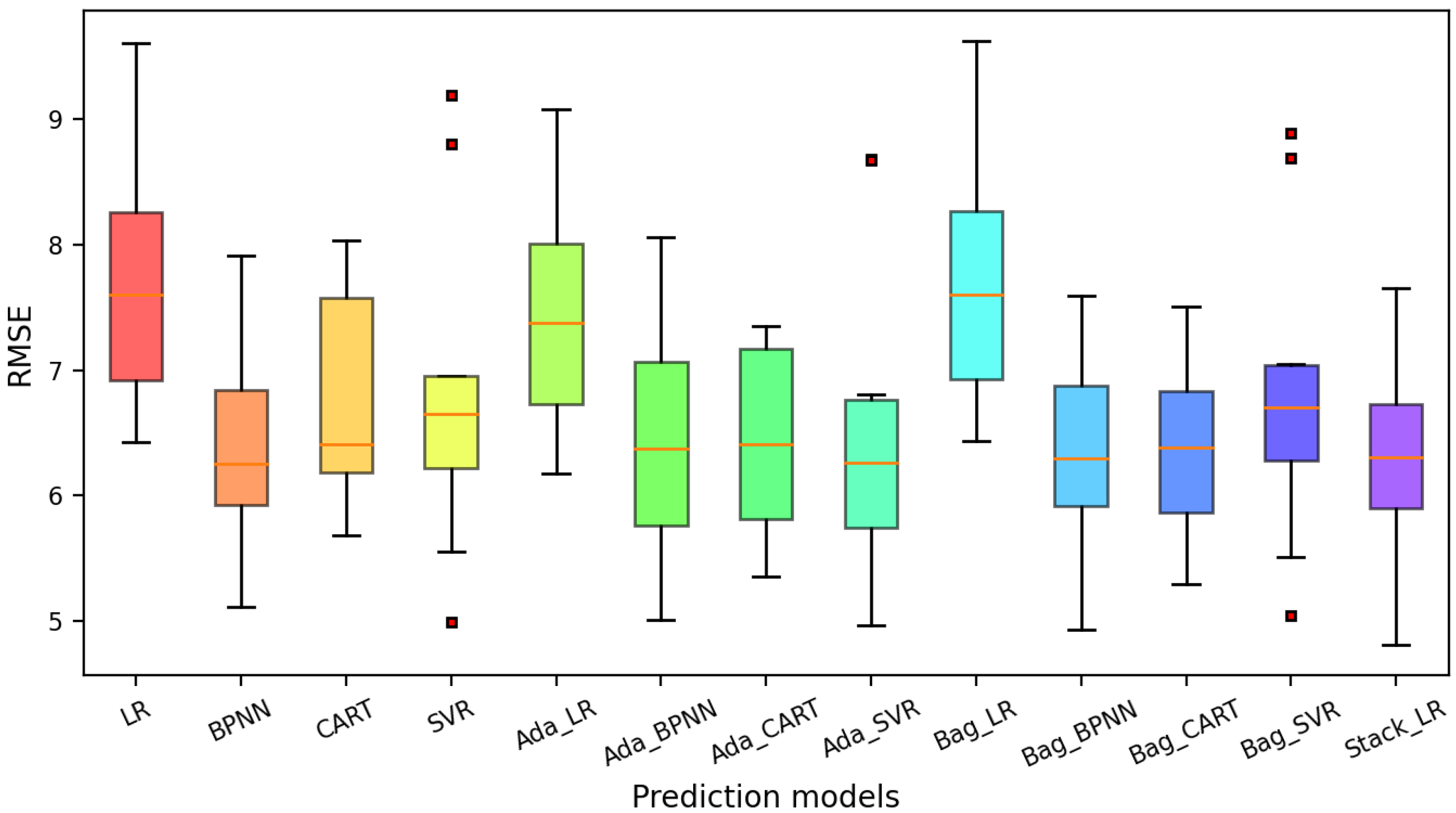
5.2.2. Comparison of the RMSE
5.3. Limitations of Application
6. Conclusions
- Among all individual ML models, the BPNN model performed the best in terms of the RMSE and , while the SVR model had the best performance in terms of the MAE;
- All ensemble methods can generally improve the prediction accuracy of individual methods; however, the improvement varies. It was found that the bagging method mainly enhanced the performance of the BPNN and CART, whereas the AdaBoost method brought a considerable improvement for the LR and SVR models;
- Among all the ML models studied, the Stack_LR model demonstrated great prediction on the self-healing of ECC and performed the best on the MAE, RMSE, and . The assessment of the box plot also revealed that the stackLR model outperformed all other models because of its shortest IQR length and smallest RMSE values;
- For the initial crack widths less than 60 m, the variations shown in the SVR model were smaller than those presented in other models. However, the CART model showed smaller variations for the crack widths between 60 m and 100 m compared to the SVR and BPNN models. For crack widths larger than 100 m, the SVR model performed the best, showing the smallest variations;
- The computational results indicated that the individual and ensemble methods could be used to predict the self-healing ability of ECC. However, how to choose an appropriate base learner and ensemble method is critical. To improve the performance accuracy, researchers should employ different ensemble methods to compare their effectiveness with different ML models.
Author Contributions
Funding
Institutional Review Board Statement
Informed Consent Statement
Data Availability Statement
Conflicts of Interest
References
- Gardner, D.; Lark, R.; Jefferson, T.; Davies, R. A survey on problems encountered in current concrete construction and the potential benefits of self-healing cementitious materials. Case Stud. Constr. Mater. 2018, 8, 238–247. [Google Scholar] [CrossRef]
- Cailleux, E.; Pollet, V. Investigations on the development of self-healing properties in protective coatings for concrete and repair mortars. In Proceedings of the 2nd International Conference on Self-Healing Materials, Chicago, IL, USA, 28 June–1 July 2009; Volume 28. [Google Scholar]
- Ramadan Suleiman, A.; Nehdi, M.L. Modeling Self-Healing of Concrete Using Hybrid Genetic Algorithm–Artificial Neural Network. Materials 2017, 10, 135. [Google Scholar] [CrossRef] [PubMed]
- Tang, W.; Kardani, O.; Cui, H. Robust evaluation of self-healing efficiency in cementitious materials—A review. Constr. Build. Mater. 2015, 81, 233–247. [Google Scholar] [CrossRef]
- Edvardsen, C. Water permeability and autogenous healing of cracks in concrete. Mater. J. 1999, 96, 448–454. [Google Scholar]
- Tang, W.; Chen, G.; Wang, S. Self-healing capability of ECC incorporating with different mineral additives—A review. In Proceedings of the 3rd International RILEM Conference on Microstructre Related Durability of Cementitious Composites, Nanjing, China, 24–26 October 2016; Miao, C., Ed.; RILEM Publications SARL: Nanjing, China, 2016; pp. 668–679. [Google Scholar]
- Jacobsen, S.; Marchand, J.; Hornain, H. SEM observations of the microstructure of frost deteriorated and self-healed concretes. Cem. Concr. Res. 1995, 25, 1781–1790. [Google Scholar] [CrossRef]
- Reinhardt, H.W.; Jooss, M. Permeability and self-healing of cracked concrete as a function of temperature and crack width. Cem. Concr. Res. 2003, 33, 981–985. [Google Scholar] [CrossRef]
- Şahmaran, M.; Yaman, İ.Ö. Influence of transverse crack width on reinforcement corrosion initiation and propagation in mortar beams. Can. J. Civ. Eng. 2008, 35, 236–245. [Google Scholar] [CrossRef]
- Clear, C. The Effects of Autogenous Healing Upon the Leakage of Water Through Cracks in Concrete; Technical Report; Wexham Spring: Buckinghamshire, UK, 1985. [Google Scholar]
- Sahmaran, M.; Yildirim, G.; Erdem, T.K. Self-healing capability of cementitious composites incorporating different supplementary cementitious materials. Cem. Concr. Compos. 2013, 35, 89–101. [Google Scholar] [CrossRef] [Green Version]
- Kamada, T.; Li, V.C. The effects of surface preparation on the fracture behavior of ECC/concrete repair system. Cem. Concr. Compos. 2000, 22, 423–431. [Google Scholar] [CrossRef]
- Li, V.C.; Kanda, T. Innovations forum: Engineered cementitious composites for structural applications. J. Mater. Civ. Eng. 1998, 10, 66–69. [Google Scholar] [CrossRef] [Green Version]
- Özbay, E.; Šahmaran, M.; Lachemi, M.; Yücel, H.E. Self-Healing of Microcracks in High-Volume Fly-Ash-Incorporated Engineered Cementitious Composites. ACI Mater. J. 2013, 110, 33. [Google Scholar]
- Wu, M.; Johannesson, B.; Geiker, M. A review: Self-healing in cementitious materials and engineered cementitious composite as a self-healing material. Constr. Build. Mater. 2012, 28, 571–583. [Google Scholar] [CrossRef]
- Huang, H.; Ye, G.; Damidot, D. Characterization and quantification of self-healing behaviors of microcracks due to further hydration in cement paste. Cem. Concr. Res. 2013, 52, 71–81. [Google Scholar] [CrossRef]
- Suleiman, A.R.; Nelson, A.J.; Nehdi, M.L. Visualization and quantification of crack self-healing in cement-based materials incorporating different minerals. Cem. Concr. Compos. 2019, 103, 49–58. [Google Scholar] [CrossRef]
- Zhou, J.; Qian, S.; Sierra Beltran, M.; Ye, G.; Schlangen, E.; van Breugel, K. Developing engineered cementitious composite with local materials. In Proceedings of the International Conference on Microstructure Related Durability of Cementitious Composites, Nanjing, China, 13–15 October 2008. [Google Scholar]
- Li, V.C.; Yang, E.H. Self healing in concrete materials. In Self Healing Materials; Springer: Dordrecht, The Netherlands, 2007; pp. 161–193. [Google Scholar]
- Zhang, Z.; Qian, S.; Ma, H. Investigating mechanical properties and self-healing behavior of micro-cracked ECC with different volume of fly ash. Constr. Build. Mater. 2014, 52, 17–23. [Google Scholar] [CrossRef]
- Yildirim, G.; Sahmaran, M.; Ahmed, H.U. Influence of hydrated lime addition on the self-healing capability of high-volume fly ash incorporated cementitious composites. J. Mater. Civ. Eng. 2014, 27, 04014187. [Google Scholar] [CrossRef]
- Yang, Y.; Lepech, M.; Li, V.C. Self-Healing of ECC under Cyclic Wetting and Drying. In Proceedings of the International Workshop of Durability of Reinforced Concrete under Combined Mechanical and Climatic Loads (CMCL), Qingdao, China, 27–28 October 2005. [Google Scholar]
- Sahmaran, M.; Li, M.; Li, V.C. Transport properties of engineered cementitious composites under chloride exposure. ACI Mater. J. 2007, 104, 604. [Google Scholar]
- Qian, S.; Zhou, J.; Schlangen, E. Influence of curing condition and precracking time on the self-healing behavior of engineered cementitious composites. Cem. Concr. Compos. 2010, 32, 686–693. [Google Scholar] [CrossRef]
- Alshihri, M.M.; Azmy, A.M.; El-Bisy, M.S. Neural networks for predicting compressive strength of structural light weight concrete. Constr. Build. Mater. 2009, 23, 2214–2219. [Google Scholar] [CrossRef]
- Xu, H.; Zhou, J.; G Asteris, P.; Jahed Armaghani, D.; Tahir, M.M. Supervised machine learning techniques to the prediction of tunnel boring machine penetration rate. Appl. Sci. 2019, 9, 3715. [Google Scholar] [CrossRef] [Green Version]
- Reuter, U.; Sultan, A.; Reischl, D.S. A comparative study of machine learning approaches for modeling concrete failure surfaces. Adv. Eng. Softw. 2018, 116, 67–79. [Google Scholar] [CrossRef]
- Miani, M.; Dunnhofer, M.; Rondinella, F.; Manthos, E.; Valentin, J.; Micheloni, C.; Baldo, N. Bituminous Mixtures Experimental Data Modeling Using a Hyperparameters-Optimized Machine Learning Approach. Appl. Sci. 2021, 11, 11710. [Google Scholar] [CrossRef]
- Moayedi, H.; Bui, D.T.; Dounis, A.; Lyu, Z.; Foong, L.K. Predicting heating load in energy-efficient buildings through machine learning techniques. Appl. Sci. 2019, 9, 4338. [Google Scholar] [CrossRef] [Green Version]
- Gilan, S.S.; Jovein, H.B.; Ramezanianpour, A.A. Hybrid support vector regression–particle swarm optimization for prediction of compressive strength and RCPT of concretes containing metakaolin. Constr. Build. Mater. 2012, 34, 321–329. [Google Scholar] [CrossRef]
- Yan, F.; Lin, Z.; Wang, X.; Azarmi, F.; Sobolev, K. Evaluation and prediction of bond strength of GFRP-bar reinforced concrete using artificial neural network optimized with genetic algorithm. Compos. Struct. 2017, 161, 441–452. [Google Scholar] [CrossRef]
- Yaseen, Z.M.; Deo, R.C.; Hilal, A.; Abd, A.M.; Bueno, L.C.; Salcedo-Sanz, S.; Nehdi, M.L. Predicting compressive strength of lightweight foamed concrete using extreme learning machine model. Adv. Eng. Softw. 2018, 115, 112–125. [Google Scholar] [CrossRef]
- Yan, K.; Shi, C. Prediction of elastic modulus of normal and high strength concrete by support vector machine. Constr. Build. Mater. 2010, 24, 1479–1485. [Google Scholar] [CrossRef]
- Chou, J.S.; Tsai, C.F.; Pham, A.D.; Lu, Y.H. Machine learning in concrete strength simulations: Multi-nation data analytics. Constr. Build. Mater. 2014, 73, 771–780. [Google Scholar] [CrossRef]
- Sobhani, J.; Najimi, M.; Pourkhorshidi, A.R.; Parhizkar, T. Prediction of the compressive strength of no-slump concrete: A comparative study of regression, neural network and ANFIS models. Constr. Build. Mater. 2010, 24, 709–718. [Google Scholar] [CrossRef]
- Omran, B.A.; Chen, Q.; Jin, R. Comparison of data mining techniques for predicting compressive strength of environmentally friendly concrete. J. Comput. Civ. Eng. 2016, 30, 04016029. [Google Scholar] [CrossRef] [Green Version]
- Mauludin, L.M.; Oucif, C. Modeling of self-healing concrete: A review. J. Appl. Comput. Mech. 2019, 5, 526–539. [Google Scholar]
- Chaitanya, M.; Manikandan, P.; Kumar, V.P.; Elavenil, S.; Vasugi, V. Prediction of self-healing characteristics of GGBS admixed concrete using Artificial Neural Network. J. Phys. Conf. Ser. 2020, 1716, 012019. [Google Scholar] [CrossRef]
- Zhuang, X.; Zhou, S. The prediction of self-healing capacity of bacteria-based concrete using machine learning approaches. Comput. Mater. Contin. 2019, 59, 57–77. [Google Scholar] [CrossRef] [Green Version]
- Huang, X.; Wasouf, M.; Sresakoolchai, J.; Kaewunruen, S. Prediction of healing performance of autogenous healing concrete using machine learning. Materials 2021, 14, 4068. [Google Scholar] [CrossRef] [PubMed]
- Ahmad, M.; Kamiński, P.; Olczak, P.; Alam, M.; Iqbal, M.J.; Ahmad, F.; Sasui, S.; Khan, B.J. Development of Prediction Models for Shear Strength of Rockfill Material Using Machine Learning Techniques. Appl. Sci. 2021, 11, 6167. [Google Scholar] [CrossRef]
- Nasiri, S.; Khosravani, M.R. Machine learning in predicting mechanical behavior of additively manufactured parts. J. Mater. Res. Technol. 2021, 14, 1137–1153. [Google Scholar] [CrossRef]
- AS 3972-2010 General Purpose and Blended Cements. Available online: https://infostore.saiglobal.com/en-au/standards/as-3972-2010-122323_saig_as_as_268436/?gclid=Cj0KCQjw3IqSBhCoARIsAMBkTb0Ex9GHRGK_51CWoBo1ioVfTRsjLMlFR7Gt7V7PJWLzXBtybrTbPFQaAni7EALw_wcB&gclsrc=aw.ds (accessed on 30 September 2021).
- Chen, G. Repeatability of Self-Healing in ECC with Various Mineral Admixtures. Ph.D. Thesis, School of Architecture and Built Environment, University of Newcastle, Callaghan, Australia, 2021. [Google Scholar]
- Nehdi, M.; Djebbar, Y.; Khan, A. Neural network model for preformed-foam cellular concrete. Mater. J. 2001, 98, 402–409. [Google Scholar]
- Oztacs, A.; Pala, M.; Ozbay, E.; Kanca, E.; Caglar, N.; Bhatti, M.A. Predicting the compressive strength and slump of high strength concrete using neural network. Constr. Build. Mater. 2006, 20, 769–775. [Google Scholar] [CrossRef]
- Deepa, C.; SathiyaKumari, K.; Sudha, V.P. Prediction of the compressive strength of high performance concrete mix using tree based modeling. Int. J. Comput. Appl. 2010, 6, 18–24. [Google Scholar] [CrossRef]
- Duan, Z.H.; Kou, S.C.; Poon, C.S. Prediction of compressive strength of recycled aggregate concrete using artificial neural networks. Constr. Build. Mater. 2013, 40, 1200–1206. [Google Scholar] [CrossRef]
- Sun, J.; Zhang, J.; Gu, Y.; Huang, Y.; Sun, Y.; Ma, G. Prediction of permeability and unconfined compressive strength of pervious concrete using evolved support vector regression. Constr. Build. Mater. 2019, 207, 440–449. [Google Scholar] [CrossRef]
- Chen, G. Self-Healing of ECC. 2021. Available online: https://github.com/davidnsw/Self-healing-of-ECC (accessed on 1 March 2022).
- Neter, J.; Kutner, M.H.; Nachtsheim, C.J.; Wasserman, W. Applied Linear Statistical Models; Irwin: Chicago, IL, USA, 1996; Volume 4. [Google Scholar]
- Cortes, C.; Vapnik, V. Support-vector networks. Mach. Learn. 1995, 20, 273–297. [Google Scholar] [CrossRef]
- Vapnik, V.N. An overview of statistical learning theory. IEEE Trans. Neural Netw. 1999, 10, 988–999. [Google Scholar] [CrossRef] [PubMed] [Green Version]
- Juncai, X.; Qingwen, R.; Zhenzhong, S. Prediction of the strength of concrete radiation shielding based on LS-SVM. Ann. Nucl. Energy 2015, 85, 296–300. [Google Scholar] [CrossRef]
- Rundo, F.; Trenta, F.; di Stallo, A.L.; Battiato, S. Machine learning for quantitative finance applications: A survey. Appl. Sci. 2019, 9, 5574. [Google Scholar] [CrossRef] [Green Version]
- Suykens, J.A.; Vandewalle, J. Least squares support vector machine classifiers. Neural Process. Lett. 1999, 9, 293–300. [Google Scholar] [CrossRef]
- Li, Y.; Shao, X.; Cai, W. A consensus least squares support vector regression (LS-SVR) for analysis of near-infrared spectra of plant samples. Talanta 2007, 72, 217–222. [Google Scholar] [CrossRef]
- Yuvaraj, P.; Murthy, A.R.; Iyer, N.R.; Sekar, S.; Samui, P. Support vector regression based models to predict fracture characteristics of high strength and ultra high strength concrete beams. Eng. Fract. Mech. 2013, 98, 29–43. [Google Scholar] [CrossRef]
- Smola, A.J.; Schölkopf, B. A tutorial on support vector regression. Stat. Comput. 2004, 14, 199–222. [Google Scholar] [CrossRef] [Green Version]
- Mukherjee, A.; Biswas, S.N. Artificial neural networks in prediction of mechanical behavior of concrete at high temperature. Nucl. Eng. Des. 1997, 178, 1–11. [Google Scholar] [CrossRef]
- Naderpour, H.; Rafiean, A.H.; Fakharian, P. Compressive strength prediction of environmentally friendly concrete using artificial neural networks. J. Build. Eng. 2018, 16, 213–219. [Google Scholar] [CrossRef]
- Yi, D.; Ahn, J.; Ji, S. An effective optimization method for machine learning based on ADAM. Appl. Sci. 2020, 10, 1073. [Google Scholar] [CrossRef] [Green Version]
- Breiman, L. Classification and Regression Trees; Routledge: London, UK, 2017. [Google Scholar]
- Dan, S.; Colla, P. CART: Tree-Structured Non-Parametric Data Analysis; Salford Systems: San Diego, CA, USA, 1995. [Google Scholar]
- Put, R.; Perrin, C.; Questier, F.; Coomans, D.; Massart, D.; Vander Heyden, Y. Classification and regression tree analysis for molecular descriptor selection and retention prediction in chromatographic quantitative structure–retention relationship studies. J. Chromatogr. A 2003, 988, 261–276. [Google Scholar] [CrossRef]
- Frosyniotis, D.; Stafylopatis, A.; Likas, A. A divide-and-conquer method for multi-net classifiers. Pattern Anal. Appl. 2003, 6, 32–40. [Google Scholar] [CrossRef]
- Dietterich, T.G. Ensemble methods in machine learning. In Proceedings of the International Workshop on Multiple Classifier Systems, Cagliari, Italy, 21–23 June 2000; Springer: Berlin/Heidelberg, Germany, 2000; pp. 1–15. [Google Scholar]
- Breiman, L. Bagging predictors. Mach. Learn. 1996, 24, 123–140. [Google Scholar] [CrossRef] [Green Version]
- Freund, Y.; Schapire, R.E. Experiments with a New Boosting Algorithm. In Proceedings of the International Conference on Machine Learning, Bari, Italy, 3–6 July 1996; Volume 96, pp. 148–156. [Google Scholar]
- Raschka, S. MLxtend: Providing machine learning and data science utilities and extensions to Python’s scientific computing stack. J. Open Source Softw. 2018, 3, 638. [Google Scholar] [CrossRef]
- Sill, J.; Takács, G.; Mackey, L.; Lin, D. Feature-weighted linear stacking. arXiv 2009, arXiv:0911.0460. [Google Scholar]
- Stacking. StackingCVRegressor-mlxtend. Available online: https://rasbt.github.io/mlxtend/user_guide/regressor/StackingCVRegressor/ (accessed on 4 March 2022).
- Kohavi, R. A study of cross-validation and bootstrap for accuracy estimation and model selection. In Proceedings of the International Joint Conference on Artificial Intelligence, Montreal, QC, Canada, 20–25 August 1995; Volume 14, pp. 1137–1145. [Google Scholar]
- Dor, O.; Zhou, Y. Achieving 80% ten-fold cross-validated accuracy for secondary structure prediction by large-scale training. Proteins Struct. Funct. Bioinform. 2007, 66, 838–845. [Google Scholar] [CrossRef]
- Nguyen, H.; Vu, T.; Vo, T.P.; Thai, H.T. Efficient machine learning models for prediction of concrete strengths. Constr. Build. Mater. 2021, 266, 120950. [Google Scholar] [CrossRef]
- Herbert, E.N.; Li, V.C. Self-Healing of Microcracks in Engineered Cementitious Composites (ECC) under a Natural Environment. Materials 2013, 6, 2831–2845. [Google Scholar] [CrossRef]
- Liu, H.; Zhang, Q.; Gu, C.; Su, H.; Li, V. Influence of microcrack self-healing behavior on the permeability of Engineered Cementitious Composites. Cem. Concr. Compos. 2017, 82, 14–22. [Google Scholar] [CrossRef]
- De Belie, N.; Gruyaert, E.; Al-Tabbaa, A.; Antonaci, P.; Baera, C.; Bajare, D.; Darquennes, A.; Davies, R.; Ferrara, L.; Jefferson, T.; et al. A review of self-healing concrete for damage management of structures. Adv. Mater. Interfaces 2018, 5, 1800074. [Google Scholar] [CrossRef]
- Taffese, W.Z.; Sistonen, E.; Puttonen, J. CaPrM: Carbonation prediction model for reinforced concrete using machine learning methods. Constr. Build. Mater. 2015, 100, 70–82. [Google Scholar] [CrossRef]
- Olalusi, O.B.; Spyridis, P. Machine learning-based models for the concrete breakout capacity prediction of single anchors in shear. Adv. Eng. Softw. 2020, 147, 102832. [Google Scholar] [CrossRef]
- Contributors, W. Root-Mean-Square Deviation—Wikipedia, The Free Encyclopedia. 2021. Available online: https://en.wikipedia.org/wiki/Root-mean-square_deviation (accessed on 28 August 2021).
- UON. Getting Started with HPC. 2021. Available online: https://www.newcastle.edu.au/events/research-and-innovation/hpc (accessed on 1 March 2022).


| Chemical Composition (%) | GPC | FA | LP | SF |
|---|---|---|---|---|
| Silica (SiO) | 19.8 | 65.90 | 1.8 | 95.10 |
| Alumina (AlO) | 5.3 | 24.0 | 0.5 | 0.21 |
| Iron oxide (FeO) | 3.0 | 2.87 | 0.6 | 0.29 |
| Calcium oxide (CaO) | 64.2 | 1.59 | 72.0 | - |
| Magnesia (MgO) | 1.3 | 0.42 | 1.0 | - |
| RO | 0.6 | 1.93 | - | - |
| Sulfur trioxide (SO) | 2.7 | - | - | - |
| Titanium oxide (TiO) | 0.28 | 0.91 | - | - |
| Manganic oxide (MnO) | 0.22 | - | - | - |
| Zirconia (ZrO) + Hafnium (HfO) | - | - | - | 3.46 |
| Loss on ignition (%) | 2.8 | 1.53 | 24.0 | 1.4 |
| Density (g/cm) | 3.08 | 2.43 | 2.25 | 2.26 |
| Specific surface area (m/kg) | - | 655 | 460 |
| Length | Length/ | Young’s Modulus | Elongation | Tensile Strength | Density |
|---|---|---|---|---|---|
| (mm) | Diameter Ratio | (MPa) | (%) | (MPa) | (g/cm) |
| 8 | 200 | 42,000 | 7 | 1600 | 1.3 |
| Mix | Water/cm | Sand | Water | Fiber (V) | GPC | Fly Ash | SF | LP | HRWR |
|---|---|---|---|---|---|---|---|---|---|
| FA70 | 0.29 | 419.67 | 338.07 | 26 | 349.73 | 816.03 | 0.00 | - | 5.13 |
| FA65-SF5 | 0.29 | 419.67 | 338.07 | 26 | 349.73 | 757.74 | 58.29 | - | 5.13 |
| FA60-SF10 | 0.29 | 419.67 | 338.07 | 26 | 349.73 | 699.45 | 116.58 | - | 5.13 |
| FA55-SF15 | 0.29 | 419.67 | 338.07 | 26 | 349.73 | 641.16 | 174.86 | - | 5.13 |
| FA65-LP5 | 0.29 | 419.67 | 338.07 | 26 | 349.73 | 757.74 | - | 58.29 | 5.13 |
| FA60-LP10 | 0.29 | 419.67 | 338.07 | 26 | 349.73 | 699.45 | - | 116.58 | 5.13 |
| FA55-LP15 | 0.29 | 419.67 | 338.07 | 26 | 349.73 | 641.16 | - | 174.86 | 5.13 |
| FA55-SF5-LP10 | 0.29 | 419.67 | 338.07 | 26 | 349.73 | 641.16 | 58.29 | 116.58 | 5.13 |
| FA55-SF10-LP5 | 0.29 | 419.67 | 338.07 | 26 | 349.73 | 641.16 | 116.58 | 58.29 | 5.13 |
| Mix | Number of Cracks | Crack Width before Self-Healing | Crack Width after Self-Healing | ||
|---|---|---|---|---|---|
| Min (m) | Max (m) | Min (m) | Max (m) | ||
| FA70 | 87 | 3.28 | 134.69 | 0 | 121.37 |
| FA65-SF5 | 77 | 4.37 | 135.47 | 0 | 124.01 |
| FA60-SF10 | 88 | 5.18 | 121.78 | 0 | 113.11 |
| FA55-SF15 | 88 | 3.45 | 115.8 | 0 | 109.53 |
| FA65-LP5 | 112 | 7.65 | 119.45 | 0 | 105.65 |
| FA60-LP10 | 37 | 5.62 | 126.82 | 0 | 110.97 |
| FA55-LP15 | 61 | 6.42 | 132.65 | 0 | 115.95 |
| FA55-SF5-LP10 | 34 | 8.74 | 123.09 | 0 | 110.78 |
| FA55-SF10-LP5 | 33 | 4.64 | 131.57 | 0 | 119.79 |
| Models | MAE | RMSE | |||||
|---|---|---|---|---|---|---|---|
| Individual models | LR | 5.012 | - | 7.680 | - | 0.860 | - |
| BPNN | 4.329 | −13.6 | 6.515 | −15.2 | 0.899 | 4.5 | |
| CART | 4.305 | −14.1 | 6.811 | −11.3 | 0.887 | 3.1 | |
| SVR | 4.296 | −14.3 | 6.826 | −11.1 | 0.883 | 2.7 | |
| Ensemble models | Ada_LR | 4.784 | −4.6 | 7.400 | −3.6 | 0.867 | 0.8 |
| Ada_BPNN | 4.226 | −15.7 | 6.435 | −16.2 | 0.900 | 4.7 | |
| Ada_CART | 4.207 | −16.1 | 6.455 | −15.9 | 0.898 | 4.4 | |
| Ada_SVR | 4.145 | −17.3 | 6.577 | −14.4 | 0.893 | 3.8 | |
| Bag_LR | 5.014 | 0.0 | 7.689 | 0.1 | 0.860 | 0.0 | |
| Bag_BPNN | 4.143 | −17.3 | 6.341 | −17.4 | 0.901 | 4.8 | |
| Bag_CART | 4.093 | −18.3 | 6.358 | −17.2 | 0.901 | 4.8 | |
| Bag_SVR | 4.302 | −14.2 | 6.820 | −11.2 | 0.883 | 2.7 | |
| Stack_LR | 3.934 | −21.5 | 6.118 | −20.3 | 0.904 | 5.1 |
| Benchmark | Model | MAE | RMSE | Benchmark | Model | MAE | RMSE | ||
|---|---|---|---|---|---|---|---|---|---|
| LR | Ada_LR | −4.6 | −3.6 | 0.8 | LR | Bag_LR | 0.0 | 0.1 | 0.0 |
| BPNN | Ada_BPNN | −2.4 | −1.2 | 0.1 | BPNN | Bag_BPNN | −4.3 | −2.7 | 0.2 |
| CART | Ada_CART | −2.3 | −5.2 | 1.2 | CART | Bag_CART | −4.9 | −6.6 | 1.6 |
| SVR | Ada_SVR | −3.5 | −3.6 | 1.1 | SVR | Bag_SVR | 0.1 | −0.1 | 0.0 |
| Ada_LR | Stack_LR | −17.8 | −17.3 | 4.3 | Bag_LR | Stack_LR | −21.5 | −20.4 | 5.1 |
Publisher’s Note: MDPI stays neutral with regard to jurisdictional claims in published maps and institutional affiliations. |
© 2022 by the authors. Licensee MDPI, Basel, Switzerland. This article is an open access article distributed under the terms and conditions of the Creative Commons Attribution (CC BY) license (https://creativecommons.org/licenses/by/4.0/).
Share and Cite
Chen, G.; Tang, W.; Chen, S.; Wang, S.; Cui, H. Prediction of Self-Healing of Engineered Cementitious Composite Using Machine Learning Approaches. Appl. Sci. 2022, 12, 3605. https://doi.org/10.3390/app12073605
Chen G, Tang W, Chen S, Wang S, Cui H. Prediction of Self-Healing of Engineered Cementitious Composite Using Machine Learning Approaches. Applied Sciences. 2022; 12(7):3605. https://doi.org/10.3390/app12073605
Chicago/Turabian StyleChen, Guangwei, Waiching Tang, Shuo Chen, Shanyong Wang, and Hongzhi Cui. 2022. "Prediction of Self-Healing of Engineered Cementitious Composite Using Machine Learning Approaches" Applied Sciences 12, no. 7: 3605. https://doi.org/10.3390/app12073605
APA StyleChen, G., Tang, W., Chen, S., Wang, S., & Cui, H. (2022). Prediction of Self-Healing of Engineered Cementitious Composite Using Machine Learning Approaches. Applied Sciences, 12(7), 3605. https://doi.org/10.3390/app12073605