Application of the Harmony Search Algorithm for Optimization of WDN and Assessment of Pipe Deterioration

Abstract

The relevance of the optimal design of water distribution networks lies in its applicability. Thus, the design must be as efficient and affordable as possible, meaning that it achieves a minimum level of serviceability using an appropriate amount of resources. In this context, an ideal water network requires the use of minimum-size elements to reach the minimum head pressure required for each node of the system with the lowest energy consumption. For this purpose, a relatively new meta-heuristic algorithm, called Harmony Search, was used in this study to optimize the water distribution network of Cheongna International City, Korea, in terms of the pipe diameter. Furthermore, using the same algorithm under a different approach, an assessment of the deterioration of conduits over time was conducted by analyzing the optimal roughness coefficient for the original pipe material, which provides a useful tool for decision making. Other heuristic and meta-heuristic algorithms have been applied to this type of problem; however, Harmony Search provides a convenient implementation at a reasonable computational cost. In this study, Harmony Search is demonstrated to be a valuable tool for water distribution network optimization as well as for pipe aging assessment.

1. Introduction

One of the primary objectives for the sustainable development of today’s societies is to guarantee access to drinking water for the entire population. Considering climate change and its consequences, the design of infrastructures, both current and future, must be as efficient and sustainable as possible. This means that they must be capable of meeting their intended service requirements with the lowest possible energy consumption, and at the lowest possible cost.

In this sense, the ideal design for water distribution networks is one in which the water inside the entire system flows by gravity because it is not necessary to provide external energy so that the water reaches all supply points. This means avoiding the need to install pumping stations to increase the water head pressure, which implies significant energy and cost savings. In other words, the design of the infrastructure must be optimal in terms of construction and operation.

The main objective of this study was to optimize the water distribution network of Cheongna International City in the Korea. For this purpose, the Harmony Search (HS) algorithm [1] was implemented to determine the optimal pipe diameter considering the required limitations on the head pressure in the nodes and the flow velocity in the pipe network. The pipe diameter was chosen to be the main element for optimization because of its high impact on water flow followed by the roughness coefficient and conduit length [2]. In this manner, the aim of this optimization process was to reduce the pressure inside the water distribution network to avoid problems related to leakage and the quick deterioration of the elements of the system due to high pressure.

The second part of this research was to find the critical conduits in the system by applying the same HS algorithm scheme using a different approach. This consists of using the C value of the roughness coefficient as the parameter to be optimized in the objective function, applied to the original water distribution network (WDN). Therefore, the outcomes of this approach provide the C value range that should be maintained in order to maintain the desired level of serviceability in the system. Consequently, conduits exhibiting higher values of C can be identified as the critical pipes that should be substituted in the first term as the WDN ages. Therefore, as the Cheongna International City WDN is formed by ductile iron pipes, whose C value can be assumed to decrease by a factor of ten every 10 years [3], the objective of this part of the study was to provide a useful tool for decision making in the assessment of deteriorated pipes.

The implementation of the HS algorithm was carried out using the EPANET-MATLAB Toolkit [4], an open-source software tool that allows EPANET to interface with MATLAB. This tool allows the user to integrate the governing equations and functions of EPANET using different mathematical approaches for WDN optimization. Some of the different approaches used by other researchers include linear programming (LP) [5,6], simulated annealing (SA) [7,8], and genetic algorithms (GAs) [8,9]. However, the HS algorithm was chosen for this study because of its relatively new meta-heuristic approach that encompasses convenient implementation and rapid convergence with reasonable computational cost [1,10,11,12,13].

The structure of this paper begins with a brief review of the theoretical background needed to conduct this experiment (use of the HS algorithm and EPANET), followed by a description of the study area, discussion of the model construction, presentation and discussion of the results, and the conclusions and future work.

2. Theoretical Background

2.1. Harmony Search Algorithm

Harmony Search (HS) is a relatively new meta-heuristic algorithm based on the improvisation process followed by musicians to find a pleasing harmony [1]. It possesses several advantages over the traditional optimization techniques: (1) it is a simple meta-heuristic algorithm that does not require an initial setting for decision variables; (2) it uses stochastic random searches, so derivative information is not necessary; and (3) it has a few parameters for fine tuning [13]. For these reasons, HS has been demonstrated in several studies to be a useful optimization algorithm for various engineering applications owing to its convenient implementation, rapid convergence, and reasonable computational cost. This can be conveniently found in the literature as applications to continuous and discrete optimization problems [14,15,16,17,18,19].

The concept of HS is based on the idea that during the improvisation process, musicians try different combinations of familiar (memorized) pitches, which is analogous to the optimization process applied to most engineering problems. Therefore, a feasible solution is called a harmony, and each decision variable corresponds to a note, which generates a value for finding the global optimum.

The HS algorithm consists of the following steps [1]:

• Initialize the problem and algorithm parameters:

The optimization problem is defined as

$$\mathrm{Minimize} \left(\mathrm{or} \mathrm{maximize}\right)f\left(x\right)$$

(1)

$$\mathrm{Such} \mathrm{that} L{B}_i\le x_i\le U{B}_i$$

(2)

where $f\left(x\right)$ is the objective function and $x$ is a candidate solution consisting of $N$ decision variables $x_i$. $L{B}_i$ and $U{B}_i$ are the lower and upper bounds for each decision variable, respectively. In addition, the parameters of HS are the Harmony Memory Size (HMS), Harmony Memory Considering Rate (HMCR), pitch adjustment rate (PAR), bandwidth (bw), and the number of improvisations (NI) (the stopping criterion).

2.

Initialize the Harmony Memory

The Harmony Memory (HM) is a memory location where the solution vectors are stored, and is similar to the genetic pool in a GA [1,20]. The initial HS is generated from a uniform distribution of ranges, filling a matrix with a quantity of randomly generated solution vectors equal to the HMS.

$$x_i^l=L{B}_i+Rand\mathrm{x}\left(U{B}_i-L{B}_i\right), l=1,2,\dots HMS$$

(3)

3.

Improvise a new harmony

The generation of a new harmony is called improvisation. This new harmony vector, $x^{\prime }=\left(x_1^{\prime },x_2^{\prime },\dots ,x_N^{\prime }\right)$, is generated based on three rules: memory consideration, pitch adjustment, and random selection.

4.

Update the Harmony Memory

If the new vector is better than the worst harmony vector in the HM in terms of the objective function value, and no identical harmony vector is already stored in the HM, the new harmony is included in the HM, and the existing worst harmony is excluded.

5.

Check the Stopping Criterion

The algorithm terminates when the maximum number of improvisations is reached. Otherwise, Steps 3 and 4 are repeated.

2.2. EPANET

EPANET is open-source software that was developed by the US Environmental Protection Agency (EPA) in 1994 to model the hydraulics and water quality dynamics of water distribution systems. EPANET was designed as a research tool to better understand the dynamics of drinking water constituents, taking into account bulk flow and pipe wall reactions [4]. EPANET conducts simulations considering a geometric representation of a pipe network, along with a set of initial conditions (e.g., water levels in tanks) and rules on how the system is operated, and uses this information to compute flows, pressures, and water quality (e.g., disinfectant concentrations and water age) throughout the network for a certain period of time.

EPANET model pipes are links that convey water from one point in the network to another, and are assumed to be full at all times. The flow direction is from the higher hydraulic head (internal energy per weight of water) point to the lower head point. The principal hydraulic input parameters for the pipes are the start and end nodes, diameter, length, roughness coefficient (for determining head loss), and current status. Then, the computed outputs for the pipes include the flow rate, velocity, head loss, and friction factor.

The hydraulic head lost by water flowing in a pipe due to friction with the pipe walls can be computed using one of three different formulas given by Hazen–Williams, Darcy–Weisbach, and Chezy–Manning. The Hazen–Williams formula cannot be used for liquids other than water and was originally developed for turbulent flow only. The Darcy–Weisbach formula is the most theoretically correct, and applies over all flow regimes and to all liquids. The Chezy–Manning formula is more commonly used for open-channel flow.

Each formula uses the following equation to compute the head loss between the start and end nodes of the pipe:

$$h_L=A{q}^B$$

(4)

where $h_L=$ head loss (Length), $q=$ flow rate (volume/time), $A=$ the resistance coefficient, and $B=$ the flow exponent.

Table 1. Resistance coefficient and flow exponent values for each head loss formula in EPANET.

Formula	Resistance Coefficient (A)	Flow Exponent (B)
Hazen–Williams	$4.727C^{-1.852}{d}^{-4.871}L$	$1.852$
Darcy–Weisbach	$0.0252f\left(ϵ,d,q\right)d^{-5}L$	$2$
Chezy–Manning	$4.66n^2{d}^{-5.33}L$	$2$

lists the expressions for the resistance coefficient and values for the flow exponent for each of the formulas. Each formula uses a different pipe roughness coefficient, which must be empirically determined.

In the table, C = Hazen–Williams roughness coefficient, $ϵ$ = Darcy–Weisbach roughness coefficient, f = friction factor, n = Manning roughness coefficient, d = pipe diameter, L = pipe length, and q = flow rate.

From a software engineering viewpoint, EPANET is used within procedural programs through a series of direct calls to its library. This requires the user to be aware of all the different functions offered by EPANET (as well as the sequence of function calls) in order to successfully implement a simulation cycle.

To solve this difficulty, an open-source software package was developed to interface EPANET with the MATLAB technical computing language, called the EPANET-MATLAB Toolkit [3]. This software uses an object-oriented approach by defining a MATLAB Class, which provides a standardized way to handle the network structure, to call all functions as well as procedures using multiple functions to simulate and, in general, perform different types of analyses in the network through the corresponding object.

3. Study Area

The Incheon Free Economic Zone (IFEZ), located in Incheon, Korea, is a Korean Free Economic Zone officially designated by the Korean government in August 2003 that consists of three regions: Songdo, Cheongna, and the island of Yeongjong, with a total area of 209.38 km². The IFEZ is planned to become a self-contained living and business district by transforming these three areas into hubs for logistics, international business, leisure, and tourism in the Northeast Asian region. Thus, the IFEZ will become one of the future top three economic zones in the world.

For this research, the selected study area is Cheongna International City located on the mainland adjacent to Yeongjong Island. Cheongna is a development project built on 7.27 km² with a population of 90,000 people, constituting the Incheon Free Economic Zone along with Songdo and Yeongjong. It is being developed as an international business and leisure center, and is as a coastal city with major transportation axes connecting Yeongjong and Seoul, including Incheon International Airport Expressway, Gyeongin Expressway, and Gyeongin Ara Waterway.

Cheongna territory was built by reclamation of tidal flats carried out from 1979 to 1989 and was used as farmland in the 1990s and 2000s. In fact, the original reason for reclaiming this area was to use it as agricultural land [21]. Figure 1 is shows the location of study area.

According to the master plan, the extension is approximately 17.8 km². The planned population was 90,000, but already surpassed 100,000 in April 2019, and is expected to increase to 120,000–130,000 in the future if only apartment houses, officetels (common Korean multi-purpose buildings with residential and commercial units), townhouses, and detached houses that are currently on sale are counted. According to the June 2021 resident registration figures, the population is approximately 112,000 [21].

4. Model Construction

This section presents the procedure for the model construction used in this study, both for optimizing the pipe diameter of the WDN and the assessment of deteriorated pipes based on the roughness coefficient. For this purpose, the HS algorithm was implemented in MATLAB along with the EPANET-MATLAB Toolkit using two different approaches.

EPANET models the physical objects that constitute a distribution system as well as their operational parameters. Networks consist of pipes, nodes (pipe junctions), pumps, valves, and storage tanks or reservoirs. The characteristics and descriptions of these objects are stored in “Network” (.net) or “input” (.inp) files, which can also be modified by text editors or other programs such as Excel. In the case of the study area, the characteristics of the Cheongna pipe network were provided by the Incheon Metropolitan City Technical Report 2015 through an input file.

Table 2. Main characteristics of the Cheongna WDN model.

No. of Junctions	No. of Reservoirs	No. of Pipes	Roughness Coefficient C	Flow Units	Head Loss Formula
152	1	200	100	CMD	Hazen-Williams

and

Table 3. Hydraulic characteristics of the Cheongna WDN model.

Min. Ø (mm)	Max. Ø (mm)	Average Ø (mm)	Min. Hydraulic Head (m)	Max. Hydraulic Head (m)	Min. Flow Velocity (m/s)	Max. Flow Velocity (m/s)	Average Flow Velocity (m/s)
80	900	244.15	32.83	65.51	0	2.35	0.35

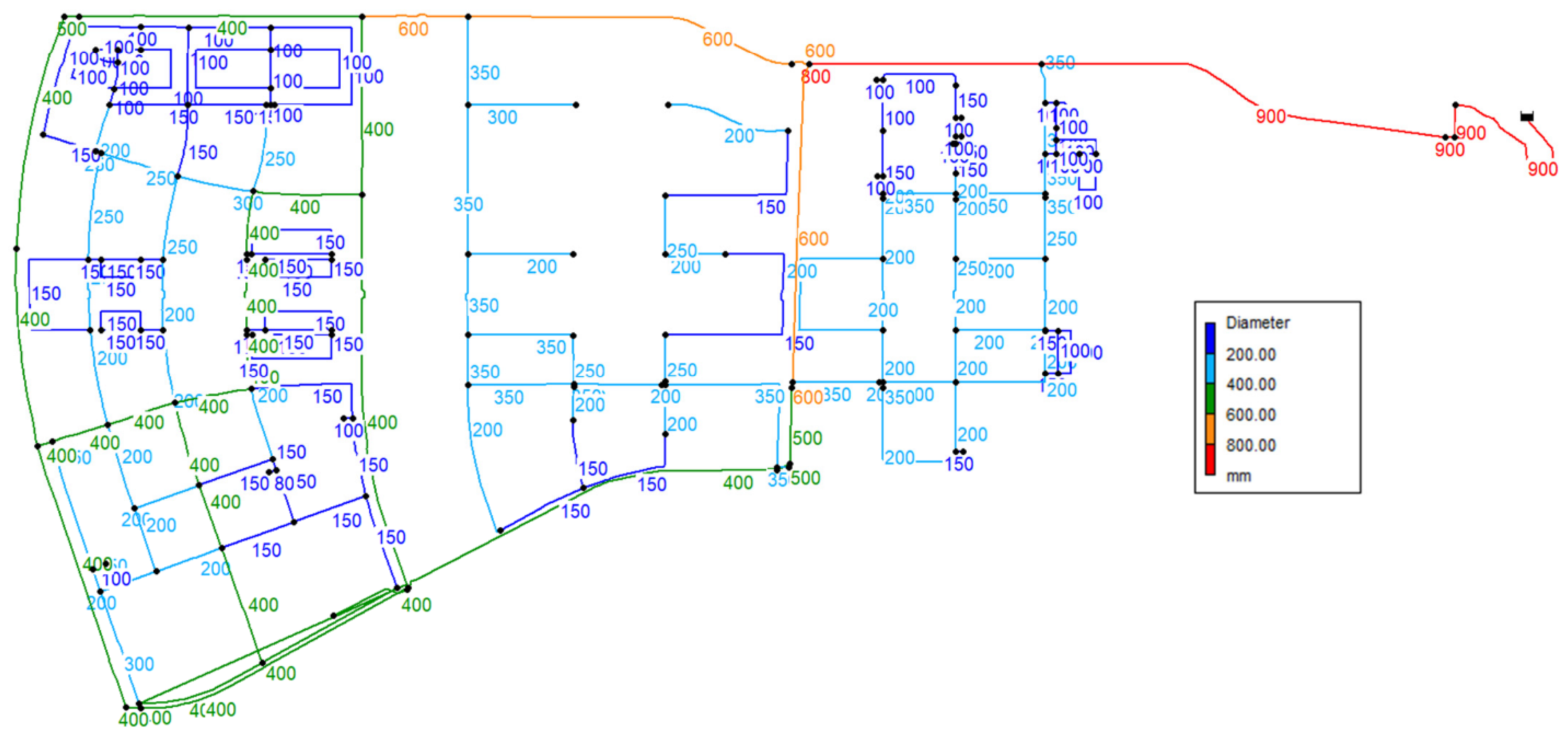
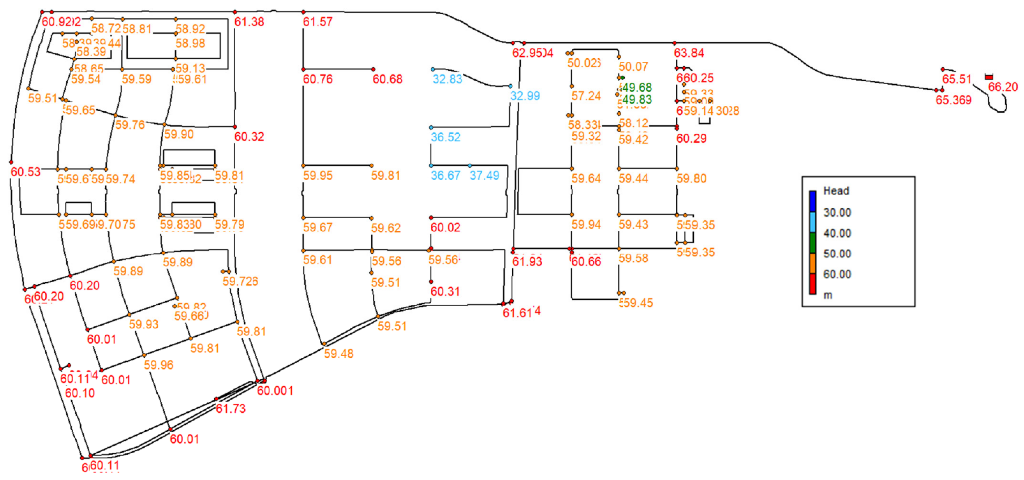
list the main aspects and hydraulic characteristics of the Cheongna WDN, respectively. Figure 2 shows the pipe size distribution of the WDN. Figure 3 shows the distribution of the hydraulic head pressure in the nodes.

4.1. Pipe Diameter Optimization

Prior to initializing the algorithm, some considerations must be taken into account. In terms of pipe diameter, the optimization of the water network implies finding the smallest diameter that is capable of providing the expected service. This means that at every junction, a minimum head pressure has to be reached, but a maximum value should also be considered according to the local standard regulations. In the case of the study area, the minimum and maximum values for the head pressures are 15.3 m and 71 m, respectively. However, in this study, a lower range of values (between 15 m and 40 m) was considered to achieve an optimal design in which the pressure in the system is reduced to avoid future leakage problems while also reaching a minimum suitable service value.

In addition to the considerations for the head pressure, a range of minimum and maximum water velocities in the pipes was also regulated for the WDN. The reason for this regulation is to guarantee a stable level of water quality regardless of the demand pattern to avoid different problems related to chlorine decay. In this case, the velocity range was established to be between 0.05 and 3 m/s.

Both head pressure and velocity limitations were used as the constraints—i.e., the penalties—in the objective function used in the HS algorithm.

4.2. Assessment of Deteriorated Pipes

To analyze the effect of pipe deterioration over time, the previous program was used, but a different approach was applied. In this case, the aim is to find the optimal C value that should be maintained across the entire system in order to maintain the original required level of serviceability. In this case, the HS algorithm can provide the distribution of the roughness coefficient for every conduit in the network, making it possible to identify those pipes that will affect the head pressure values in the nodes if they deteriorate. Therefore, the conduits exhibiting higher values of C can be assumed to be the most sensitive to pipe aging, and should be repaired or replaced in the first term.

5. Results and Discussion

Different approaches for both optimization of the WDN and assessment of deteriorated pipes were used in this study, and the results are shown and discussed below.

5.1. Determination of Optimal Pipe Diameter Set

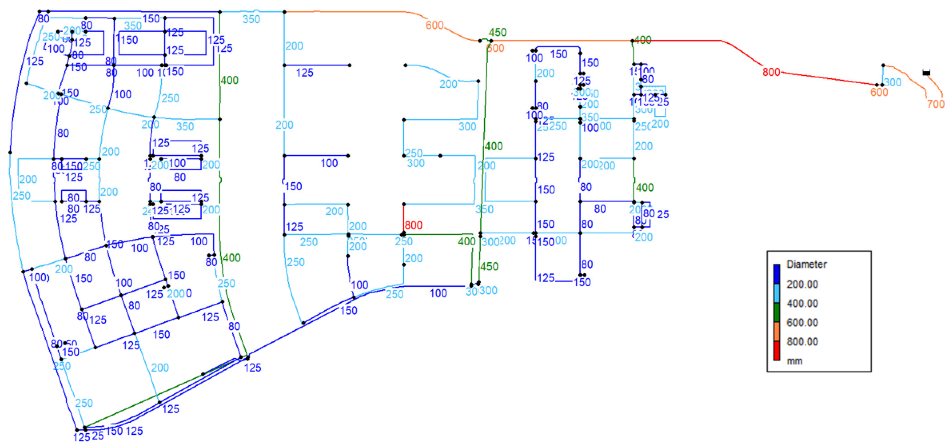
The outcomes of the application of the HS algorithm provide a set of pipe diameters that is considered to be optimal based on the constraints imposed on the objective function. These constraints, as explained in the model construction section, guide the optimization process based on the limitations of head pressure on the nodes and the flow velocity in the pipes. For this reason, although most of the conduit sizes are reduced, some of them can be increased owing to hydraulic requirements.

Table 4. Parameter settings for the HS algorithm and constraints on the objective function.

NI	HMS	HMCR	PAR	Bw	H (m)	V (m/s)
30,000	30	0.95	0.3	0.01	15–40	0.05–3

shows the parameters used for the HS algorithm as well as the objective function constraints.

In addition, before initializing the HS, it is necessary to set the upper and lower bounds between which the HS will find the solution for the optimization problem. In this case, both the upper and lower bounds were established as 80 mm and 900 mm, respectively. These values also correspond to the maximum and minimum pipe diameters that were initially set in the original model.

However, if only the lower and upper bound are specified, the HS will blindly find continuous values within this range of sizes. Thus, a set of discrete commercial pipe diameters must be established to obtain real-world applicable solutions.

Table 5. Set of commercial diameters for ductile iron pipes.

Commercial Pipe Diameters (mm)
80 100 125 150 200 250 300 350 400 450 500 600 700 800 900

shows the set of commercial pipe diameters that are common in Korea for ductile iron, which was the material considered in this study.

Although some of the conduits have increased in diameter owing to hydraulic requirements, a reduction in the average size of the pipes is achieved, providing a general reduction in the head pressure in the system, which was the main objective.

Thus, an average reduction of the maximum pipe diameter from 900 mm to 800 mm is obtained along with a reduction of the average pipe diameter of approximately 25% (from 244.15 mm in the original model to 186.9 mm in the simulated one) using the HS algorithm.

In the case of the hydraulic head, owing to the restrictions imposed as the constraints of the objective function, both the lower and upper boundaries were reduced, as expected. The minimum hydraulic head is reduced from 32.83 m in the original model to 17.46 m in the HS model. The maximum value of the hydraulic head decreases from 65.51 m in the original model to 39.06 m in the simulation. This corresponds to a reduction of approximately 50% in the lower bound and 40% in the upper bound for the hydraulic head range in the system. In this manner, the outcomes achieved by means of the HS algorithm along with the setting of the objective function have led to an optimization of the Cheongna WDN in terms of a reduction in the pressure in the system along with a reduction in the pipe diameter of the conduit network. Therefore, both results imply a reduction in the probability of damage due to high pressure as well as a reduction in the construction costs of the system.

On the other hand, as the pipe diameter is generally reduced in the network, the water flow velocity consequently increases. In this case, the maximum flow velocity in the original model is 2.35 m/s and is 2.42 m/s in the HS model, representing an increase of approximately 3%. Furthermore, the average flow velocity also increases from 0.35 m/s in the original model to 0.54 m/s in the simulated model, which represents an increase of approximately 40%. Despite the increase in the flow velocity in the system, this parameter remains within the range of admissible values, as it does not exceed the 3 m/s upper bound.

Figure 4 and Figure 5, respectively, show the results of the optimization carried out by means of the HS in terms of pipe diameter and hydraulic head.

Table 6. Outcomes of the Cheongna WDN optimization after applying the HS algorithm.

Min. Ø (mm)	Max. Ø (mm)	Average Ø (mm)	Min. Hydraulic Head (m)	Max. Hydraulic Head (m)	Min. Flow Velocity (m/s)	Max. Flow Velocity (m/s)	Average Flow Velocity (m/s)
80	800	186.9	17.46	39.06	0.05	2.42	0.54

summarizes the main outcomes of this model. For clarification, in the analysis of the results the hydraulic head values of 66.2 m and 54.15 m have been excluded, which correspond to the reservoir and to a non-supplying water point, respectively.

5.2. Assessment of Pipe Deterioration

The second part of this study is the application of the HS algorithm to find the critical pipes in terms of the roughness coefficient C. For this purpose, the HS was implemented in the same manner as for the optimal pipe diameter, but the C value was used as the objective function. In this case, by loading the original Cheongna WDN model into the EPANET-MATLAB Toolkit, the optimal values of the roughness coefficient that must be maintained to provide the original level of serviceability were determined. In this manner, it is possible to identify the conduits that exhibit higher values of C, and are thus considered to be the ones that are most sensitive to pipe aging. In this case, the range of values for the HS objective function was set between 70 and 100, based on the assumption that ductile iron tends to increase its roughness coefficient by decreasing the Hazen–Williams value of C by 10 every ten years [2].

Table 7. Evolution of the Hazen–Williams C value over time for deteriorated pipes assessment.

Aging	Current	10 Years	20 Years	30 Years
C value	100	90	80	70

lists the different values as pipes age.

Figure 6 and Figure 7 show the outcomes of this approach, in which the optimal distribution of the roughness coefficient for the entire network can be observed. Those conduits that maintain a value of C = 100 are considered as critical pipes and should be repaired or replaced in the first term as the WDN ages. Thus, this approach can provide a useful tool for determining the repair or replacement of deteriorated pipes.

Then, as explained before, as the Hazen–Williams C value of ductile iron decreases by ten every 10 years, it is relatively simple to identify from the obtained results the service life of the conduits according to the required level of serviceability of the system, which in this case was set by the constraints in the nodal head pressure. In this manner, the main objective of this second part of the study is achieved by simulating a scenario in which the original set of pipe diameters is used in order to analyze the consequences of the system aging and to identify those conduits that are more sensitive to this aging. Thus, decision makers have a tool for operation management in terms of repairing or replacement of deteriorated pipes by WDN aging.

6. Conclusions

The WDN optimization problem has been of interest to many researchers in the field of water engineering. However, many studies have focused on the optimal size of the elements of the water distribution system or its location. The purpose of this study was to not only conduct simulations using the Harmony Memory algorithm for the optimal pipe diameter, but to also attempt to provide a useful tool for future operation management and decision making. Using this method, the assessment of deteriorated conduits should assist in determining whether pipes in which the roughness coefficient is high should be replaced or repaired and to evaluate the consequences of each decision.

The application of the HS algorithm along with the EPANET-MATLAB Toolkit has allowed optimization of the Cheongna WDN. In this sense, the average pipe diameter of the network achieved a reduction of approximately 25%, which implies a design with a significant reduction in construction costs. In addition, the head pressure was reduced by approximately 45% across the entire system while still providing the desired level of serviceability.

In the second part of this study, the HS algorithm was demonstrated to be a useful tool for the identification of critical pipes that are most sensitive to aging. In this case, the outcomes of the implementation of the HS provided a distribution of the roughness coefficient C for the entire pipe network that would maintain similar values of head pressure as in the original model. In this sense, some of the conduits exhibited reduced C values, but those that exhibited higher values were identified as pipes that are more likely to affect the level of serviceability due to pipe aging. Therefore, these conduits should be repaired or replaced in the first term.

In the future, additional work should be carried out to refine the outcomes of the HS algorithm. For example, the values obtained from the pipe diameter optimization in this study determine the optimal pipe size considering only the hydraulic requirements. To apply these results in a real-world case, the size of the conduits should be reduced as the distribution points are reached. An additional step could be the application of a water quality analysis to the given results.

References

- Geem, Z.W.; Kim, J.H.; Loganathan, G.V. A New Heuristic Optimization Algorithm: Harmony Search. Simulation 2001, 76, 60–68. [Google Scholar] [CrossRef]
- Kuok, K.K.; Chiu, P.C.; Ting, D.C.M. Evaluation of “C” Values to Head Loss and Water Pressure Due to Pipe Aging: Case Study of Uni-Central Sarawak. J. Water Resour. Prot. 2020, 12, 1077–1088. [Google Scholar] [CrossRef]
- Eliades, D.G.; Kyriakou, M.; Vrachimis, S.; Polycarpou, M.M. EPANET-MATLAB Toolkit: An Open-Source Software for Interfacing EPANET with MATLAB. In Proceedings of the 14th International Conference on Computing and Control for the Water Industry (CCWI), Amsterdam, The Nederland, 7–9 November 2016. [Google Scholar]
- Rossman, L.A. EPANET 2 USERS MANUAL. United States Environmental Protection Agency. 2000. Available online: https://cfpub.epa.gov/si/si_public_record_report.cfm?Lab=NRMRL&dirEntryId=95662 (accessed on 19 February 2022).
- Karmeli, D.; Gadish, Y.; Myers, S. Design of Optimal Water Distribution Networks. J. Pipeline Div. 1968, 94, 1–10. [Google Scholar] [CrossRef]
- Alperovits, E.; Shamir, U. Design of Optimal Water Distribution Systems. Water Resour. Res. 1977, 13, 885–900. [Google Scholar] [CrossRef]
- Loganathan, G.V.; Greene, J.J.; Ahn, T.J. Design Heuristic for Global Minimum Cost Water-Distribution Systems. J. Water Resour. Plan. Manag. 1995, 121, 182–192. [Google Scholar] [CrossRef]
- Simpson, A.R.; Dandy, G.C.; Murphy, L.J. Genetic Algorithms Compared to Other Techniques for Pipe Optimization. J. Water Resour. Plan. Manag. 1994, 120, 423–443. [Google Scholar] [CrossRef] [Green Version]
- Savic, D.A.; Walters, G.A. Genetic Algorithms for Least-Cost Design of Water Distribution Networks. J. Water Resour. Plan. Manag. 1997, 123, 67–77. [Google Scholar] [CrossRef]
- Askarzadeh, A.; Rashedi, E. Harmony Search Algorithm: Basic Concepts and Engineering Applications. Recent Dev. Intell. Nat.-Inspired Comput. 2017, 1–36. [Google Scholar] [CrossRef]
- Geem, Z.W.; Kim, J.H.; Loganathan, G.V. Harmony Search Optimization: Application to Pipe Network Design. Int. J. Model. Simul. 2002, 22, 125–133. [Google Scholar] [CrossRef]
- Bekdaş, G.; Cakiroglu, C.; Islam, K.; Kim, S.; Geem, Z.W. Optimum Design of Cylindrical Walls Using Ensemble Learning Methods. Appl. Sci. 2022, 12, 2165. [Google Scholar] [CrossRef]
- Cakiroglu, C.; Islam, K.; Bekdaş, G.; Kim, S.; Geem, Z.W. CO2 Emission Optimization of Concrete-Filled Steel Tubular Rectangular Stub Columns Using Metaheuristic Algorithms. Sustainability 2021, 13, 10981. [Google Scholar] [CrossRef]
- Kumar, V.; Kumar, D.; Chhabra, J.K. Effect of Harmony Search Parameters’ Variation in Clustering. Procedia Technol. 2012, 6, 265–274. [Google Scholar] [CrossRef] [Green Version]
- Vasebi, A.; Fesanghary, M.; Bathaee, S.M.T. Combined Heat and Power Economic Dispatch by Harmony Search Algorithm. Int. J. Electr. Power Energy Syst. 2007, 29, 713–719. [Google Scholar] [CrossRef]
- Tsakirakis, E.; Marinaki, M.; Marinakis, Y.; Matsatsinis, N. A Similarity Hybrid Harmony Search Algorithm for the Team Orienteering Problem. Appl. Soft Comput. 2019, 80, 776–796. [Google Scholar] [CrossRef]
- Degertekin, S.O. Optimum Design of Steel Frames Using Harmony Search Algorithm. Struct. Multidiscip. Optim. 2008, 36, 393–401. [Google Scholar] [CrossRef]
- Gao, K.Z.; Suganthan, P.N.; Pan, Q.K.; Chua, T.J.; Cai, T.X.; Chong, C.S. Discrete Harmony Search Algorithm for Flexible Job Shop Scheduling Problem with Multiple Objectives. J. Intell. Manuf. 2016, 27, 363–374. [Google Scholar] [CrossRef]
- Cheng, M.-Y.; Prayogo, D.; Wu, Y.-W.; Lukito, M.M. A Hybrid Harmony Search Algorithm for Discrete Sizing Optimization of Truss Structure. Autom. Constr. 2016, 69, 21–33. [Google Scholar] [CrossRef]
- Geem, Z.W.; Cho, Y.-H. Optimal Design of Water Distribution Networks Using Parameter-Setting-Free Harmony Search for Two Major Parameters. J. Water Resour. Plan. Manag. 2011, 137, 377–380. [Google Scholar] [CrossRef]
- Kim, C. A Study on the Development Plan of Incheon Free Economic Zone, Korea: Based on a Comparison to a Free Economic Zone in Pudong, China. Master’s Thesis, University of Oregon, Eugene, OR, USA, 2007. [Google Scholar]