1. Introduction
Recently, computer-aided engineering, such as computational fluid dynamics (CFD), finite element analysis, and multiphysics simulations using computers, has been getting a great deal of attention in various fields, such as the academic, research, and industrial sectors, owing to the rapid advancement of computational techniques. For CFD analysis, grid systems are generally used in the Eulerian frame for both structured and unstructured grids and solvers. Currently, it is common to adopt unstructured grids and solvers that discretize the governing equations using the finite volume method because of the ease of expressing complex objects. The accuracy of the unstructured grids and solvers is relatively lower than that of the structured ones despite its high computational cost. However, the stability and accuracy of CFD simulations using these methods vary depending on the quality of the grid, and it is inefficient to carry out grid-based simulations for flows such as in free surfaces with strong nonlinearity and/or movement of a body, where grids need to be deformed, deleted, or regenerated during the simulation. To enhance its efficiency, various numerical methods such as overset grid method [
1], immersed boundary method [
2], level set method [
3], and so forth have been developed for the grid-based simulations.
In contrast to the grid-based method, in which the connection information with neighboring grids must be maintained, the gridless method, also called the meshless or mesh-free method, requires only the location information and physical quantities of the computational points when approximating the spatial derivatives at the points.
There are lots of gridless methods in the literature. Among them, smoothed particle hydrodynamics (SPH) [
4], element-free Galerkin (EFG) method [
5], reproducing kernel particle method (RPKM) [
6], partition of unity [
7], hp-clouds [
8], finite point method (FPM) [
9], generalized finite difference method (GFDM) [
10], meshless local Petrov–Galerkin (MLPG) method [
11], radial basis function (RBF) method [
12,
13], and moving particle simulation (MPS) [
14] are the popular ones. These methods have been developed until recently and are being applied in various fields. The primary areas of advancement in meshfree methods are to address issues with essential boundary enforcement, numerical quadrature, and contact and large deformations [
15]. The smoothed point interpolation method [
16], smoothed finite element method [
17] and gradient smoothing method [
18] can be applied for CFD problems.
Gridless methods can be classified in several ways. According to the form of the partial differential equations, that is, the corresponding governing equations, the methods based on the weak form of the governing equations, such as EFG, RKPM, and MLPG, are generally stable and accurate but computationally expensive and require global or local meshes in the computational domain. In contrast, SPH, FPM, RBF, and MPS, which adopt strong forms of governing equations, are generally less stable and precise than the weak-form-based methods when Neumann boundary conditions are imposed [
19].
Another classification may be based on the adopting frame, that is, the way in which the flow is described. MPS and SPH, which are Lagrangian gridless methods, have been widely used for estimating the impact force in free surface flows with strong nonlinearity and for approximating the motion of a floating body [
20,
21], especially in the field of naval architecture and ocean engineering. The method introduced by Batina [
22] is a Eulerian method that has a higher accuracy for flows near a body than Lagrangian methods because the computational points do not move, and the distance between the fluid and body boundary can easily be controlled.
For fluid flows, one classification may be whether compressibility is to be considered, which depends on the flow of interest and significantly affects the numerical algorithms for CFD. For incompressible flows, the velocity and pressure are strongly coupled, and it is important to quickly and accurately solve the pressure Poisson equation with the source term as the time change of the divergence of the velocity fields. Imposing Neumann boundary conditions for pressure can be one of the causes of unstable simulations, and considering the viscous force near the wall boundary is important. CFD simulations on incompressible unsteady viscous flow adopting the Eulerian frame is of interest in this study. The recent works by EFG, RPKM, hp-clouds, FPM, GFDM, MLPG, and RBF methods applied for these simulations can be found in [
23,
24,
25,
26,
27,
28,
29].
In this study, a Eulerian gridless solver using weighted moving least squares (WMLS) is proposed and simple remedies to impose Numeann-type boundary condition efficiently and to enhance the estimation accuracy of the viscous force near a wall boundary are adopted. Benchmark simulations of two-dimensional (2D) unsteady laminar flows were performed, and the results were compared with those of experimental and other computational methods.
2. Numerical Methods
The numerical schemes and solver developed by Jeong et al. [
30] were used. The fractional step method was adopted as the simulation algorithm. The spatial differential terms in the governing equations were approximated using the WMLS method, and the second-order Adams–Bashforth method was applied for the time integration. The solution of the Poisson equation for pressure was obtained in an iterative manner based on the WMLS method. The details are explained in the following subsections.
2.1. Governing Equations
For incompressible viscous flows, the governing equations are the continuity and Navier–Stokes equations, namely Equations (1) and (2), respectively.
where
is the velocity vector,
is the density,
is the pressure, and
is the kinematic viscosity.
2.2. Cloud Composition and Weighting Function
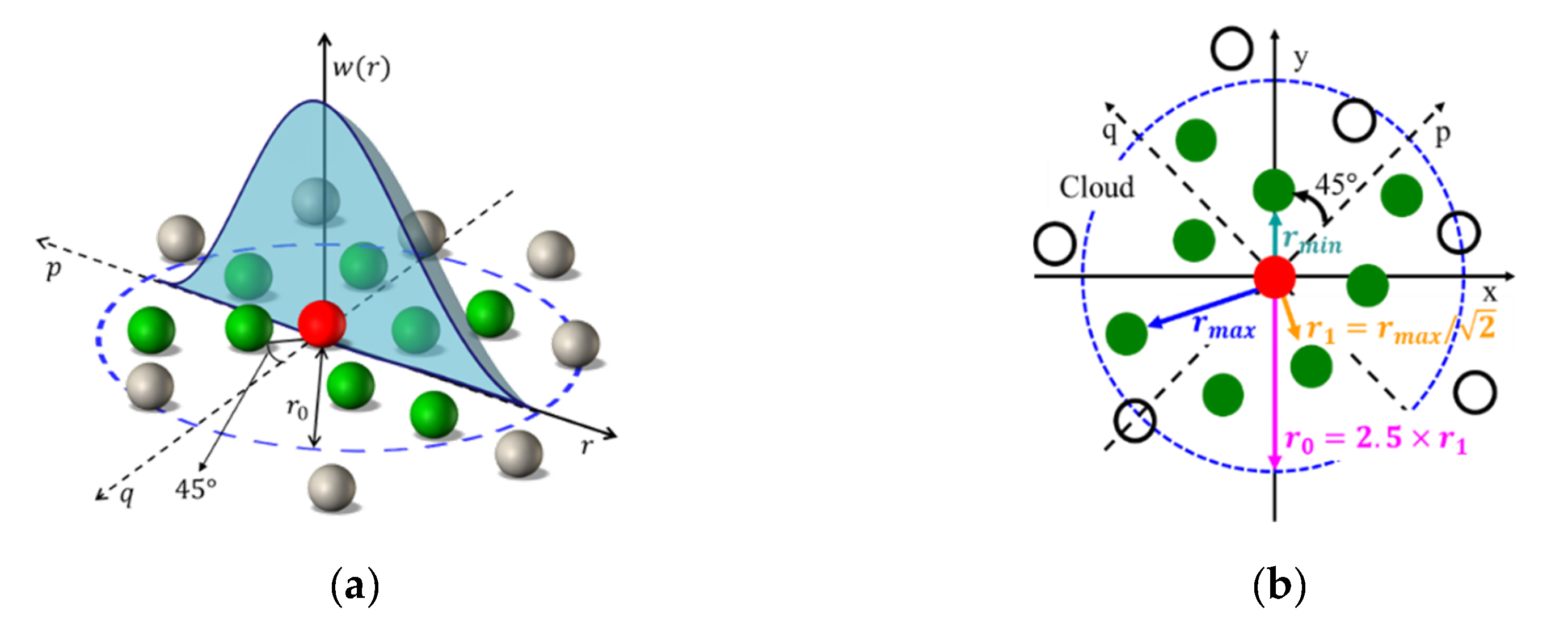
Similar to any other gridless method, it is necessary to construct clouds using neighboring computational points within a specific distance, which is called the radius of influence, kernel radius, effective radius, etc., to form a calculation point of interest. As indicated in
Figure 1a, if the points are distributed and the effective radius is
at the calculation point colored red, ten neighboring points become members of the cloud. In Lagrangian gridless methods, a constant
is generally used for all particles. However, it is not appropriate for Eulerian methods because the distances between points are not always the same, and the distances near the wall need to be shorter than in other regions. Moreover, it is desirable for the points in the cloud to be arranged in a state where information in all directions can be captured, as this reduces the adverse effect of information from points locate d far from the point of interest. To address these issues, a method [
31] that divides the cloud into quadrants was used together with a weighting function, called the kernel function, as illustrated in
Figure 1a. As shown in
Figure 1b, after finding the closest point to the calculation point, where the distance is
, the rectangular coordinate
p-q is constructed around the calculation point such that it forms an angle of 45° with the line segment between the calculation point and the closest point, and the cloud is divided into four regions. Two points were selected from each quadrant, and consequently, the cloud contained eight surrounding points. The reason for fixing the number of surrounding points to eight is to reduce the computational time and improve the efficiency by making the calculation load at each calculation point as similar as possible when developing parallelization codes in the future. Near the boundary, if two points are not included in each quadrant, the p-q coordinate system is rotated gradually to satisfy this condition. The
value was set as 2.5
, where the reference distance
is obtained by dividing the distance from the calculation point to the farthest point in the cloud by
, that is,
=
. In the case of an equally spaced distribution,
becomes
.
The weighting function used in this study is as follows:
Here, is the distance from the calculation point to the surrounding point .
2.3. Approximated Polynomials and WMLS
The WMLS-based solver developed in this study approximates the distributions of the physical quantities as a quadratic polynomial at calculation point from those of surrounding points within the effective radius of calculation point . The square of the residual between the approximated and actual values is minimized to find the coefficients of the polynomials, where the coefficients are spatial derivatives of the physical quantities.
The approximate value of the physical quantity at a neighboring point
is expressed as Equation (4) using a second-order Taylor series expansion, where
is the physical quantity of a point of interest, for example, calculation point
with coordinates
and
.
where
. Additionally, the coefficients
~
are defined as
The sum of the squares of the residual between the physical quantity assumed by this approximate polynomial expression and the actual physical quantity is obtained at all surrounding points as shown in Equation (6). Equation (7) is the minimization condition of
J. After substituting Equation (4) into Equation (6) and differentiating with respect to
~
, Equation (8) is derived.
In Equation (10), the undefined coefficients , that is, up to second-order spatial derivatives of the physical quantity, can be found if the inverse of the coefficient matrix is obtained. In particular, since each component of the coefficient matrix is expressed only by the distance between the calculation points, whether the weighting function is applied or not, the coefficient matrix and its inverse always maintain a constant value even during unsteady simulations if the distribution of the calculation points does not change. Therefore, as long as the computer memory permits, if the inverse of the coefficient matrix is obtained using conventional methods such as LU or QR decomposition in advance as preprocessing for unsteady simulations, the calculation time can be significantly reduced.
2.4. Poisson Equation
Solving the Poisson equation for the pressure is important for incompressible flows. In this study, a successive over-relaxation method in WMLS is developed and applied. The second-order differential coefficient of pressure is divided into a pressure term of a calculation point and that of the surrounding points, and the pressure is sequentially adjusted using the relaxation factor.
At each arbitrarily arranged calculation point, the convergence calculation of the pressure Poisson equation at time
, as shown in Equation (11), is performed, and the pressure field at this time is obtained. The right-side term is the time change of divergence of the fields of intermediate velocity
, which is calculated using Equation (12) from the velocity field around calculation point
.
Here, the pressure of the surrounding point
is assumed as follows:
The coefficients
~
are defined as
An expression similar to Equation (8) is derived based on the condition that the sum of the squares multiplied by the weight of the residual between the assumed pressure and the actual pressure is minimized. Splitting the terms by calculation and surrounding points, it becomes Equation (15).
Equation (15) can be expressed as follows by rearranging
and
, which correspond to the second-order spatial derivatives of the pressure used in the solution of the Poisson equation.
Here, the coefficients and can be expressed as in Equation (18). By substituting these expressions into Equation (12) and rearranging for , Equation (19) is derived, and this is updated by the relaxation method, as indicated in Equation (20).
This updated value is used for the surrounding point when the same calculation is performed at a subsequent calculation point. The update is performed in the same way for all calculation points, and the residual of the pressure
is obtained from Equation (21).
If this residual is less than or equal to the reference value, the updated pressure field is regarded as a convergence solution to the Poisson equation. However, if it exceeds the reference value, the time step is not advanced, and the pressure of the entire calculation point is updated again. For this condition, in Equations (20) and (21) is not the value in the previous time step but that of previously updated within the same time step. Thus, the convergence solution of the Poisson equation is obtained by performing iterations within the same time step.
2.5. Boundary Treatments
If a Dirichlet condition for velocity or reference pressure is imposed on any boundary in the computational domain, special treatment is not required. The velocity and pressure boundary conditions on the outer boundaries of the domain are as follows:
Here, n is the unit normal vector at the point on the boundary.
For a no-slip wall boundary, the boundary conditions for the velocity and pressure are given by Equation (23):
where
is the unit tangential vector at a point on the boundary.
A simple but efficient remedy for the Neumann-type boundary conditions in Equations (22) and (23) involves placing two computational points along the orthogonal line to the boundary points, as shown in
Figure 2. First- and second-order one-sided differencing schemes of the finite difference method are utilized for velocity and pressure, respectively. This helps to enhance the estimation accuracy of the viscous force and avoid complex treatment for constructing a cloud near the boundaries. Moreover, it will make it easy to adopt a wall function for turbulence modeling in future studies.
3. Numerical Simulations
To validate the developed solver, some typical 2D unsteady simulations of internal and external flows were performed. For the former, lid-driven cavity flows were chosen, whereas flows around a single cylinder and two circular cylinders in tandem arrangement were analyzed for the latter. The nondimensional coefficients related to the present study for all cases are the
Re and Strouhal number (
St) for the external flows.
where
,
, and
are the representative speed, length, and diameter, respectively, whereas
is the frequency of vortex shedding.
The pressure, drag, and lift coefficients used for the analysis of external flows are defined by Equations (25)–(27).
where
is an identity matrix,
is the viscous stress tensor, and
and
are the unit vectors in the
x and
y directions, respectively.
If vortex shedding occurs, the values during the last 20 periods within the simulation times are averaged, and the mean values are presented for St, , and .
3.1. Internal Flows
The lid-driven cavity problem was analyzed using the proposed method. In this problem, the fluid is contained in a square cavity consisting of three rigid walls with no-slip conditions and the lid moves with a tangential velocity on the top boundary. The kinematic viscosity was adjusted for different Re values.
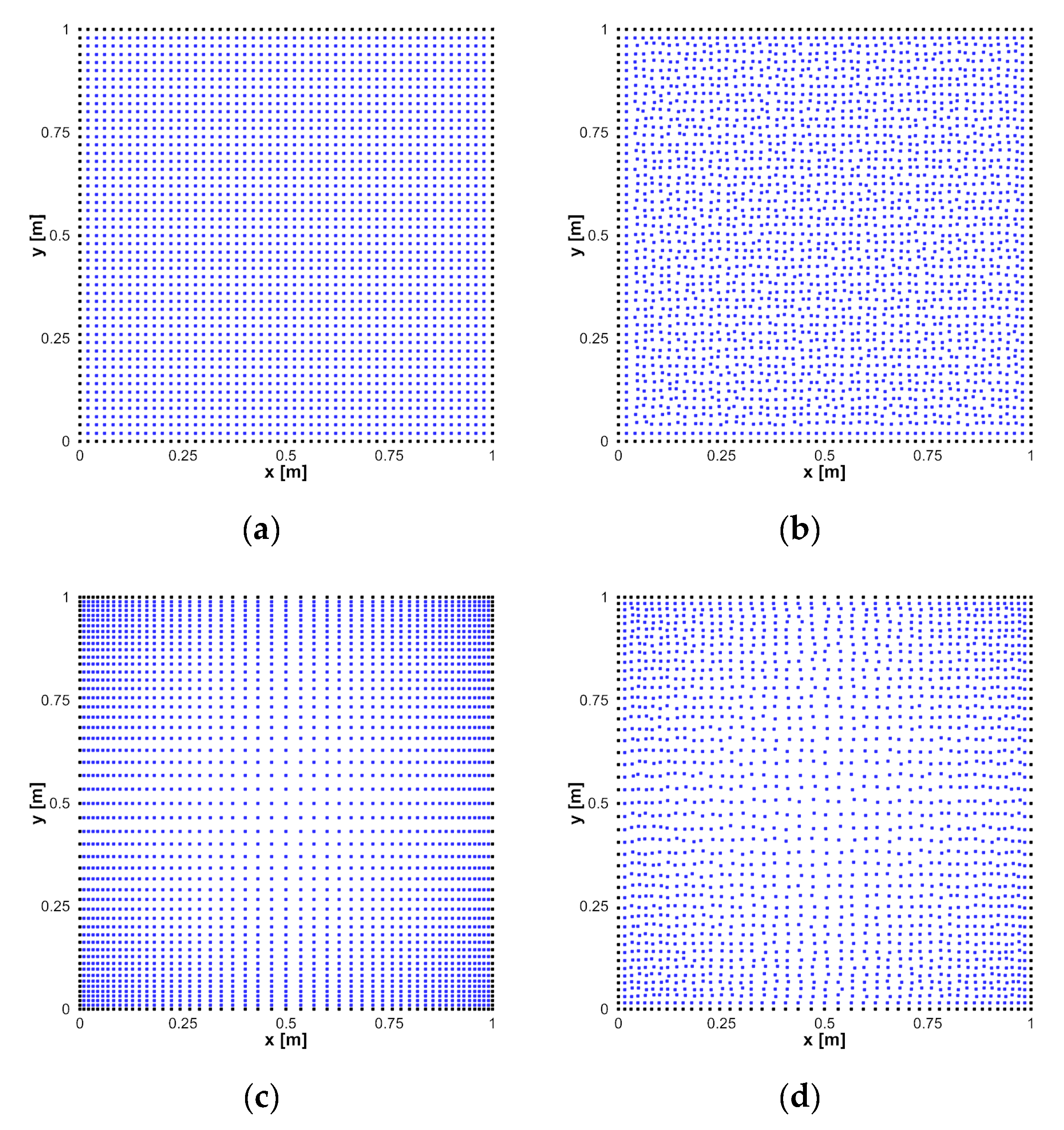
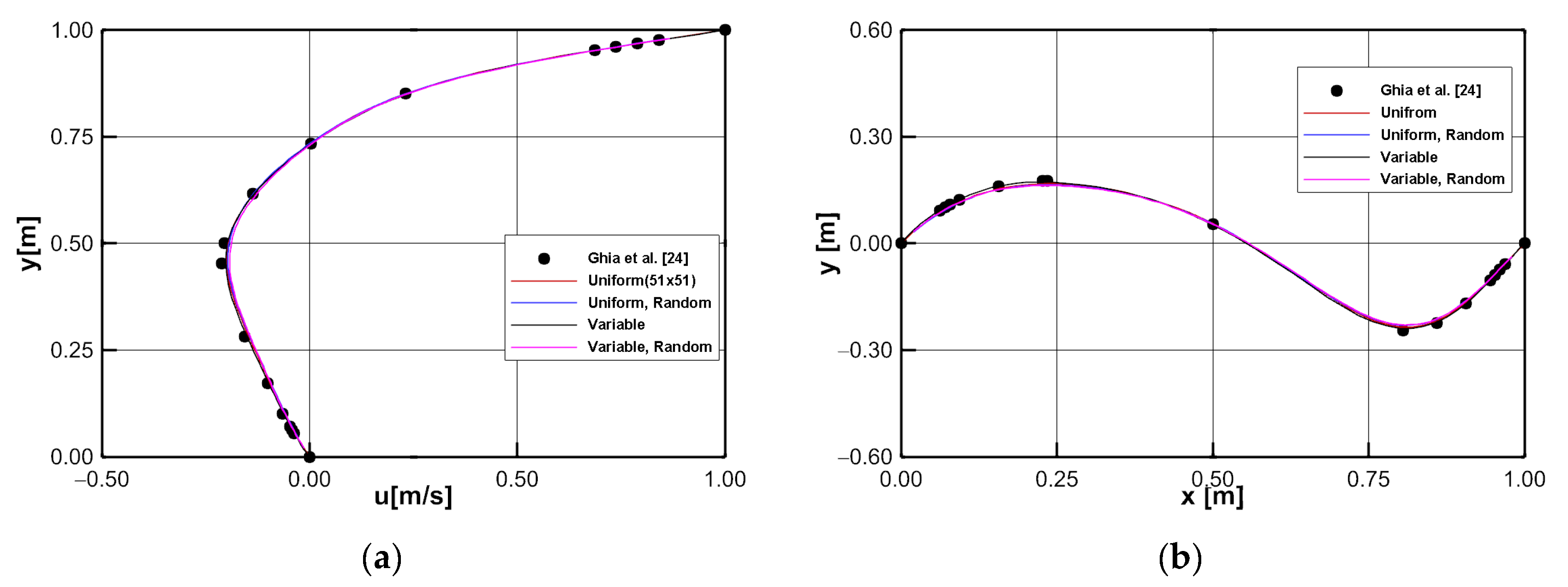
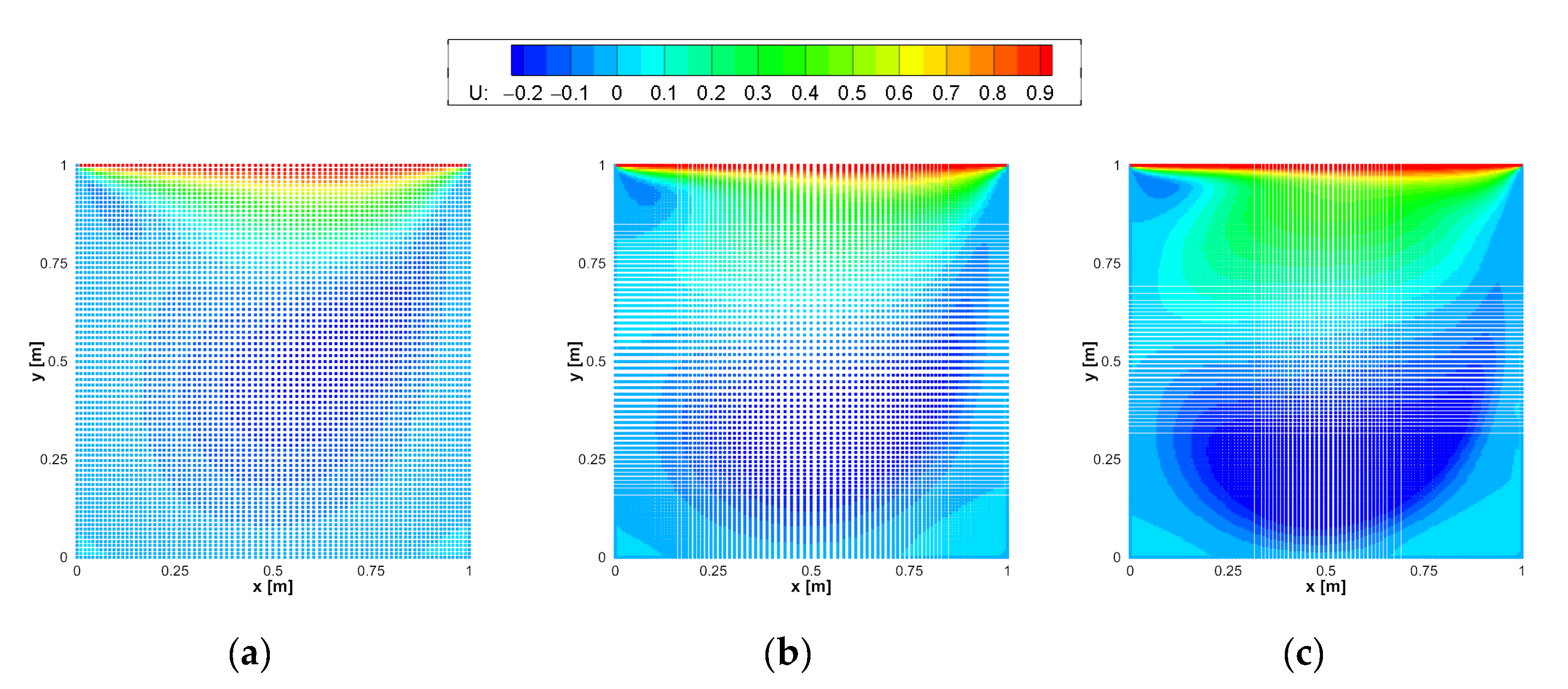
Prior to the main simulations, the effect of the distribution of the calculation points was checked. Four distributions, in which the number of points in each direction was 51, were chosen for the simulation of the cavity flows when
Re = 100, as displayed in
Figure 3. From
Figure 4, it can be observed that the velocity distributions along the central planes in the horizontal and vertical directions are similar, but the even distribution concentrated near the wall boundary shown in
Figure 3c was closer to those of the experiment [
32].
Simulations were performed for cases with
Re = 100, 400, and 1000 and 81, 101, and 151 calculation points were uniformly distributed in the horizontal (
) and vertical (
) directions, respectively. Contour maps of the velocity component in the
direction
are depicted in
Figure 5, where typical cavity flow patterns can be observed.
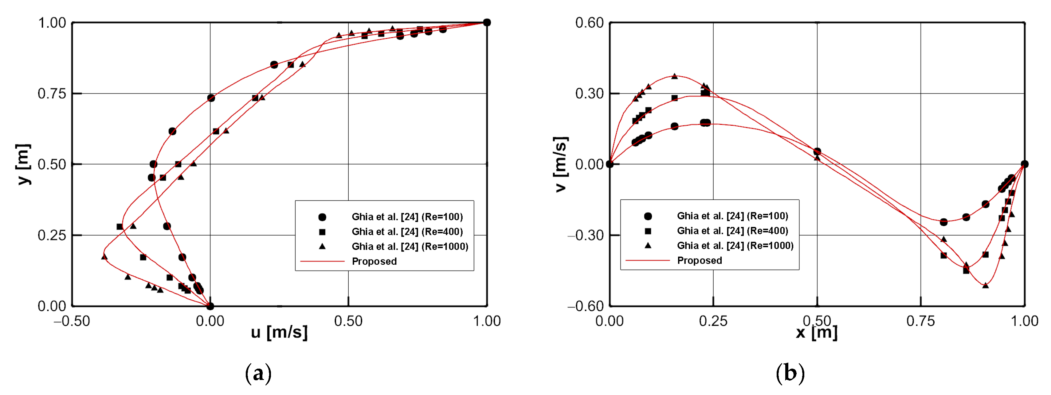
Figure 6 shows a comparison of the velocity distributions along the central planes in the horizontal and vertical directions with the experimental results. It can be seen that there is good agreement between the two.
To show the efficiency of present method, a simple comparison for the computational time was done. Since the computing speed varies greatly depending on various things, numerical simulations of cavity flow when
Re = 100 was performed by three different solvers, that is, an in-house code, icoFoam of OpenFOAM v2106, and the present one, applying only the very basic items. The CPU and operating system of the computing machine were Xeon E5-1660v3 3.0 GHz and Windows 10 pro, respectively. The in-house and present codes were compiled and linked by intel oneAPI 2021 without any optimization option in compiler level. The icoFoam was run under the environment of Ubuntu 20.04 in Window Subsystem for Linux 2. Total number of computational grids were 6400 for the grid-based solvers and that of computational points was 6651 for the present method. Time increment was 0.001 s and total simulation time was 10s. The average of elapsed time for 10 times of executions were compared in
Table 1. It can be seen that present method, which responds to the distribution of unstructured computation points, shows a computational speed similar to that of the structured solver and about 30% faster than the unstructured solver, icoFoam.
3.2. External Flows
Cylindrical structural bodies are common in nature and widely used for engineering purposes. Therefore, many studies on the fundamentals of flow around a single circular cylinder have been conducted because the existence of the cylinder results in complicated flows, vortex shedding, and changes in the hydrodynamic forces acting on it, which are significantly affected by
Re. Cylindrical structures can be found not only singly but also in groups such as fuel rods in nuclear reactors and risers of offshore plants. It can be expected that the flows are more complex in these cases owing to the interactions among them. The arrangement of two circular cylinders, which is the simplest case of a group or multiple structures, can be classified as tandem, side-by-side, or staggered ones. Previous studies have found that the flow patterns are dependent on the
Re and ratio of the distance between the centers of the two cylinders with respect to the diameter (D) of the cylinder. It has been reported that the flow characteristics and hydrodynamic forces change suddenly at a critical spacing ratio, as summarized in [
33].
In this section, the simulation results for flows around a circular cylinder under two Re values and two circular cylinders in tandem arrangement under a fixed Re value with various distances between cylinders are presented. The reason for selecting the tandem arrangement for the two cylinders is that the flows are more complicated, and a sudden drag jump is expected.
3.2.1. Single Circular Cylinder
The diameter (D) of the cylinder was 1 m, and the rectangular computational domain was set to −10D to 30D and −10D to 10D in the
x and
y directions, respectively. As for the arrangement of the calculation points, 401 and 201 points of equal intervals in the
x and
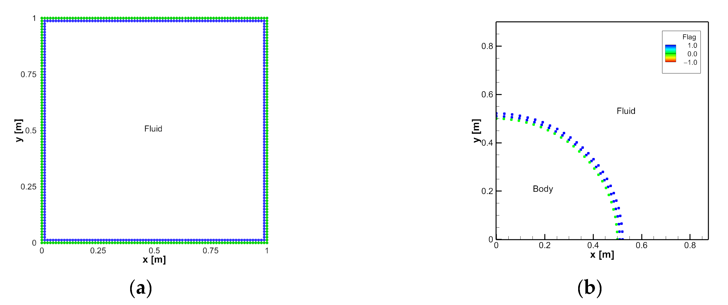
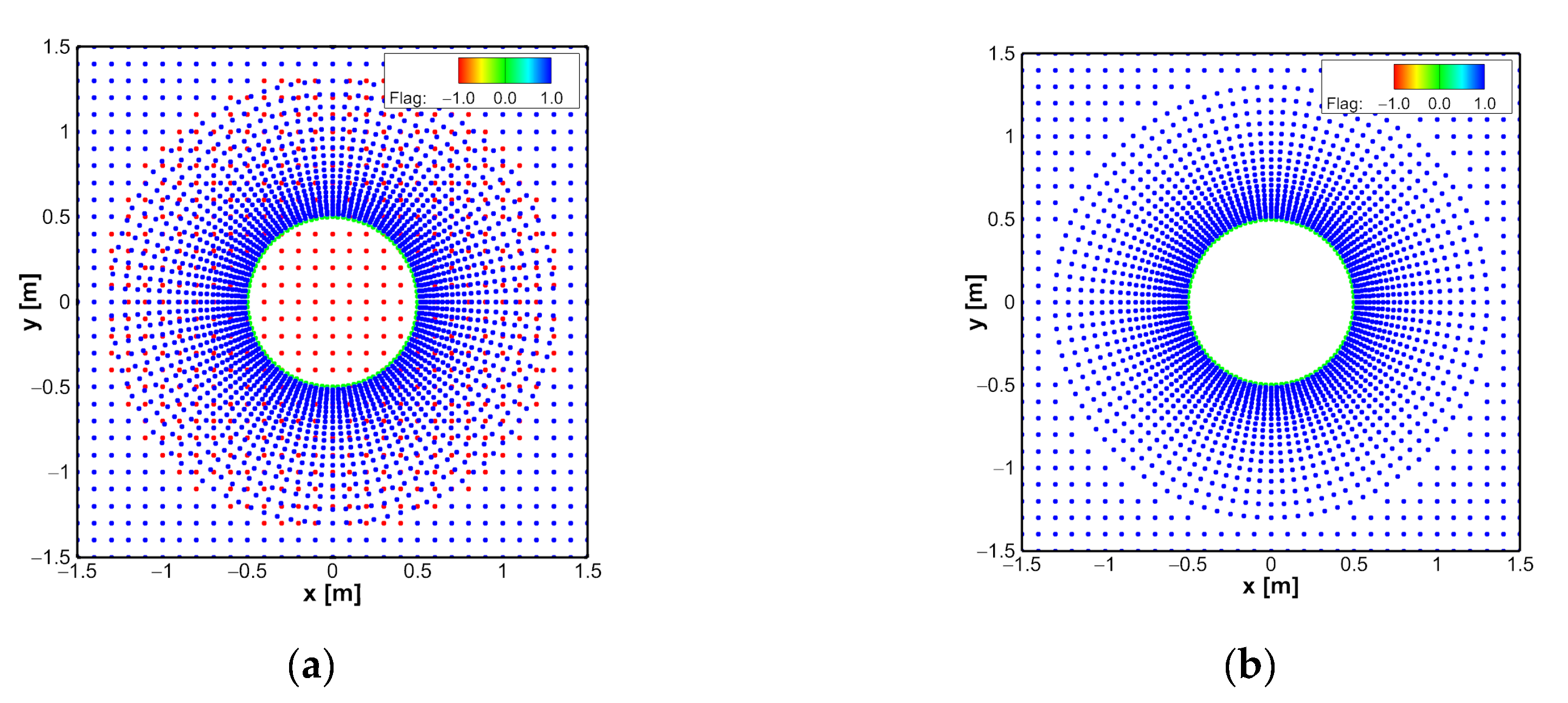
y directions were placed. For convenience, these points are hereinafter referred to as background points. Then, 101 points in the circumferential direction and 21 points concentrated around the cylinder surface in the radial direction were added. Simply put, the distributions are the same as the combination of H- and O-type structured grid systems for the entire computational domain and near the cylindrical body, respectively. Finally, the background points inside the body and those that are extremely close to the points that are not included in the background points were flagged and inactivated during the cloud construction and simulations. This method of distributing points weakens the regularity, but the authors want to show that this irregularity does not cause problems during the simulations using the proposed method. At this stage, the points in one or two layers near the boundaries were matched with the boundary points, as explained in
Section 2.5. The flagging technique was used because it is effective in dealing with problems involving single or multiple moving bodies. The cloud construction near the body was not changed, and operations were performed only for the flag-changed points and those within their effective radius.
Figure 7 shows the distribution of the computational points near a body (a) with and (b) without inactive points.
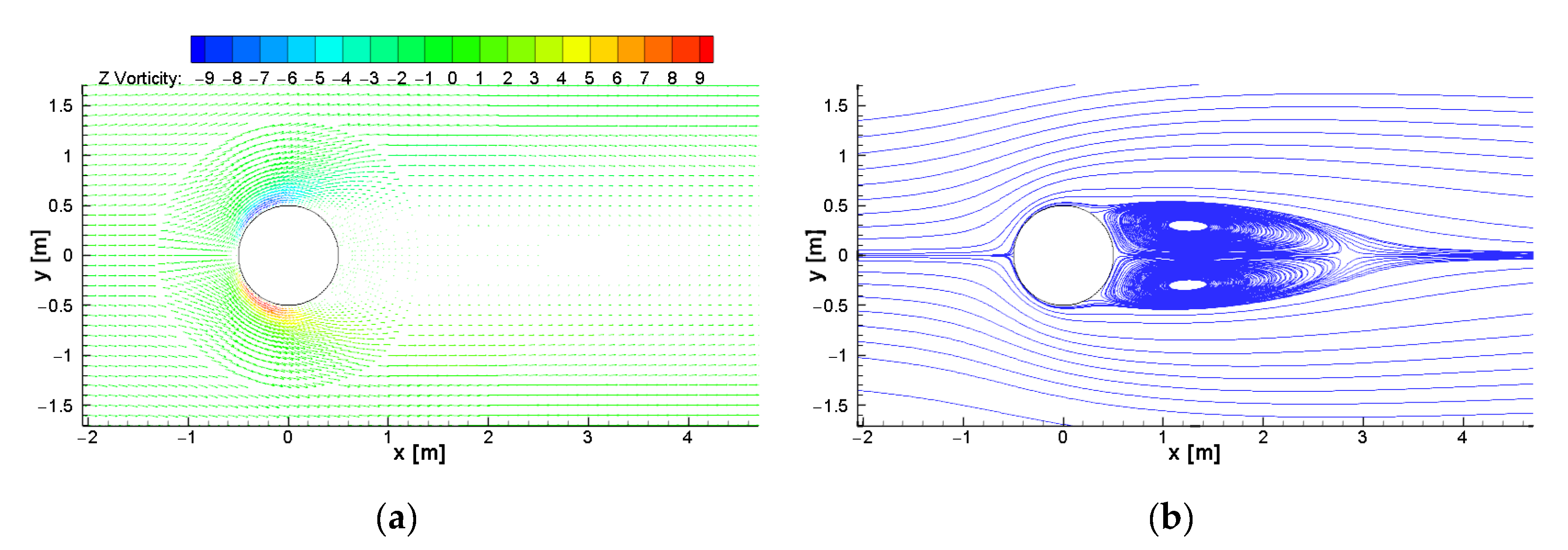
As boundary conditions for velocity, 1.0 and 0.0 m/s of velocity components u and v were applied to the inflow boundary, and a first-order Neumann condition was employed to other open boundaries. The reference pressure was zero for the top and bottom boundaries, and the Neumann condition was applied for the rest. A no-slip condition was imposed on the cylinder surface for the velocity. For the pressure boundary condition on the surface, Equation (23) was implemented. The Re value was set to 40, where vortices attached to the cylinder were observed, and 100, where periodic vortex shedding occurred. The time interval was chosen such that the Courant number is 0.5. The total simulation time was 400 s.
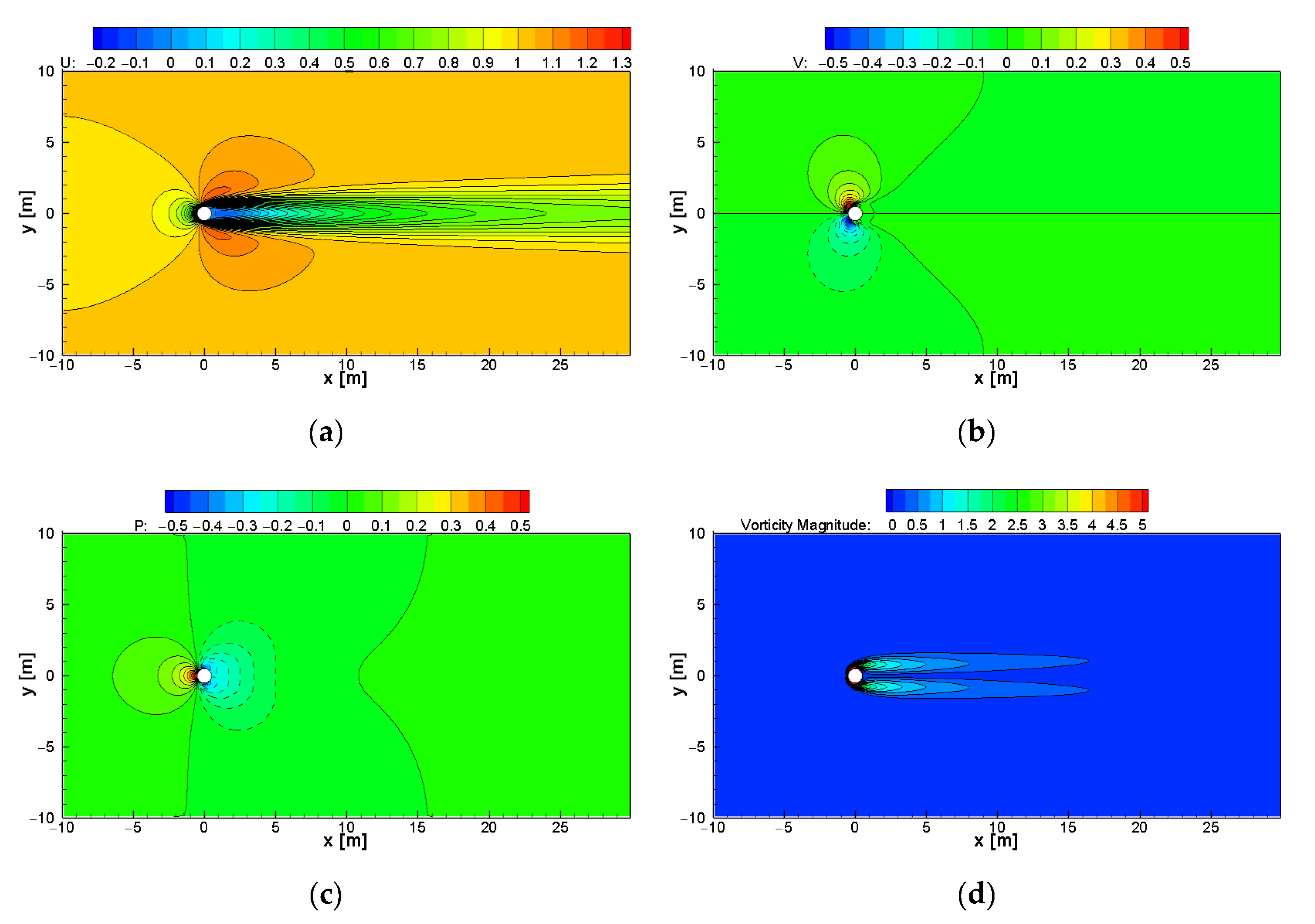
Figure 8 shows the contour maps of the velocity, pressure, and vorticity magnitude in the
x and
y directions when
Re = 40 at
t = 400 s. Symmetric flow patterns against the
y centerline of the cylinder were well reconstructed. The velocity vector fields and streamlines around the cylinder are depicted in
Figure 9. A pair of attached symmetric vortices is observed, and the attachment length of the vortex is approximately 2.3, which is in the range reported by other studies [
34,
35].
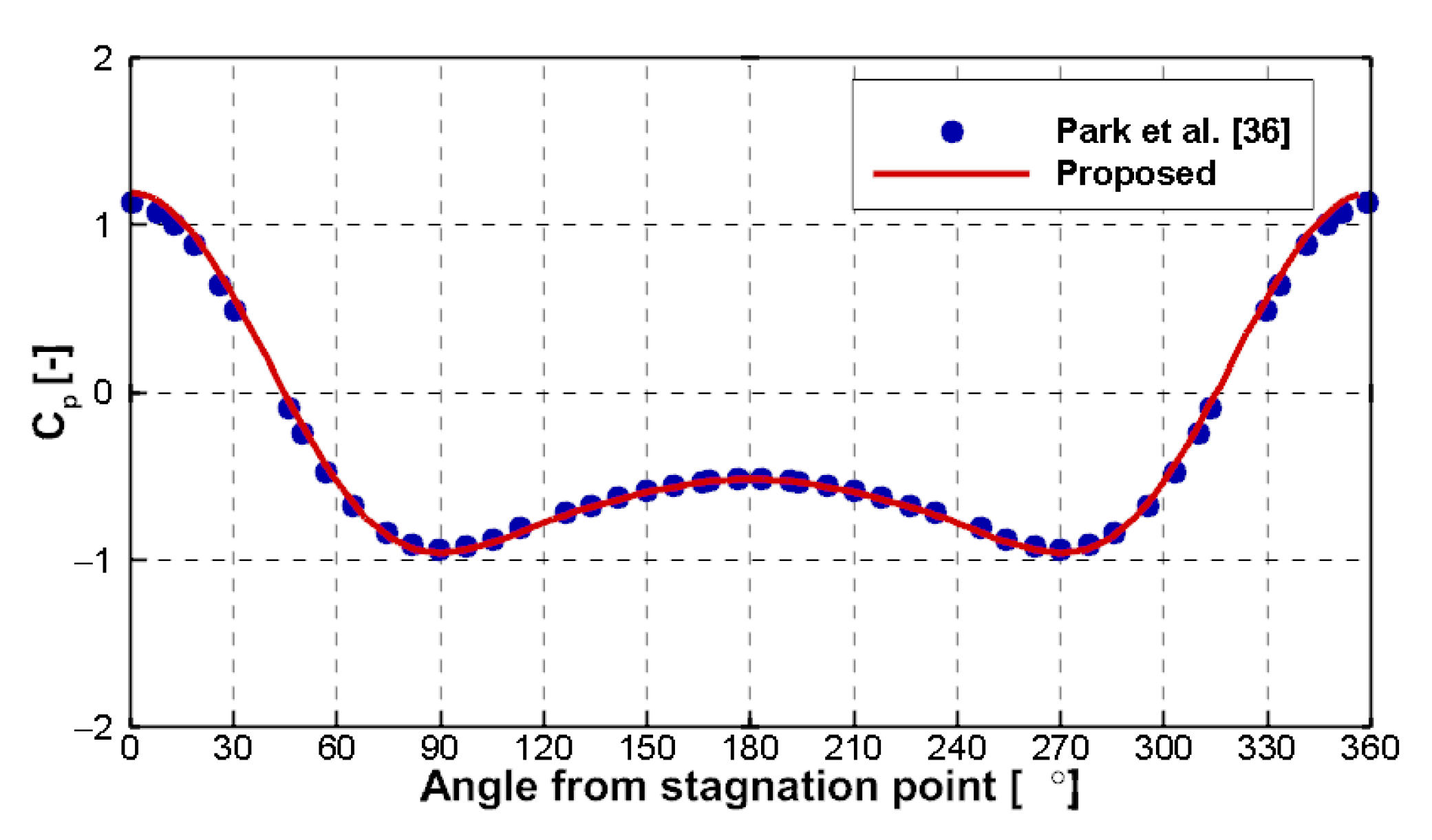
Figure 10 presents a comparison of the pressure coefficients
on the cylinder surface with the results of the methods in [
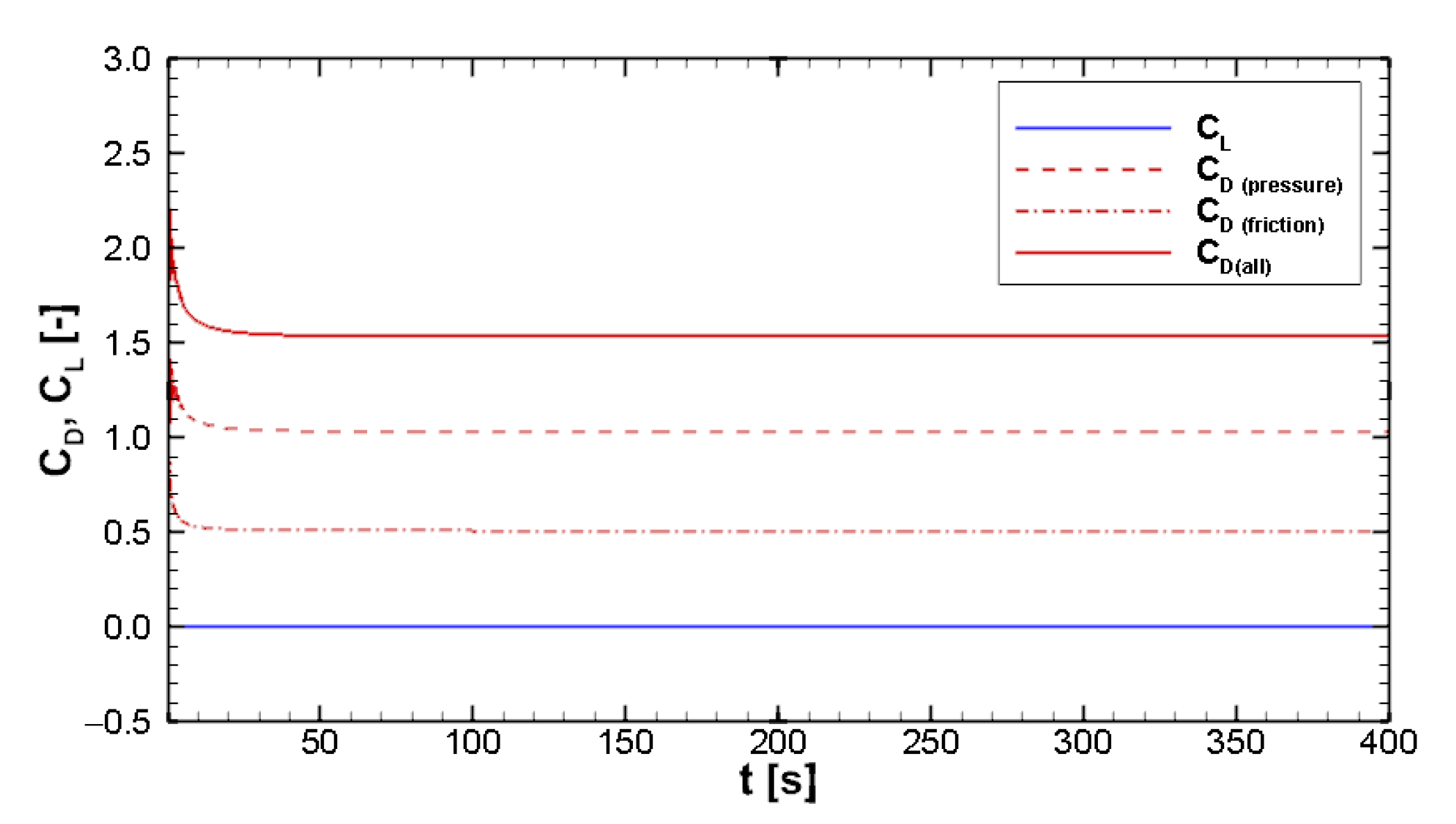
36], where good agreement can be observed. The time series of the coefficients of the hydrodynamic forces (drag and lift) are shown in
Figure 11. The coefficients converge after 50 s and the viscous forces are smaller than the pressure forces, but their magnitudes are not negligible. The drag coefficients are similar to those of the experimental and other numerical simulation results, as summarized in
Table 2.
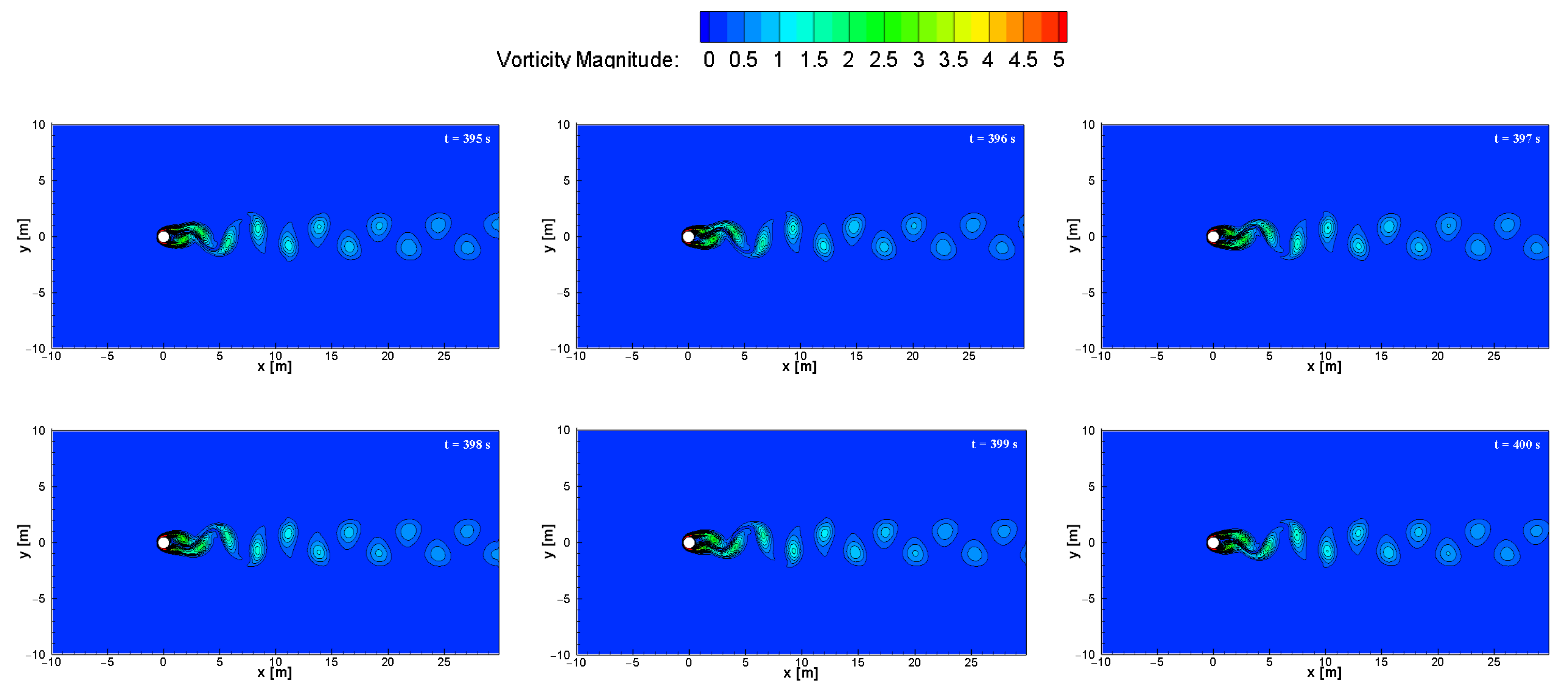
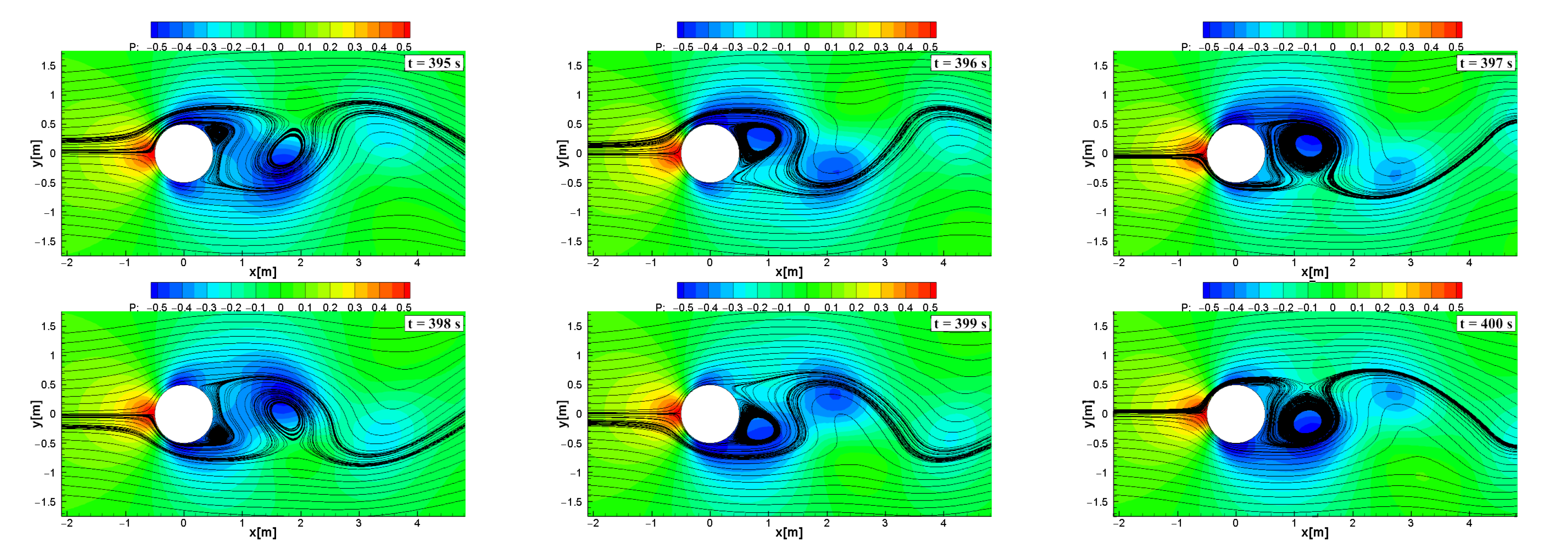
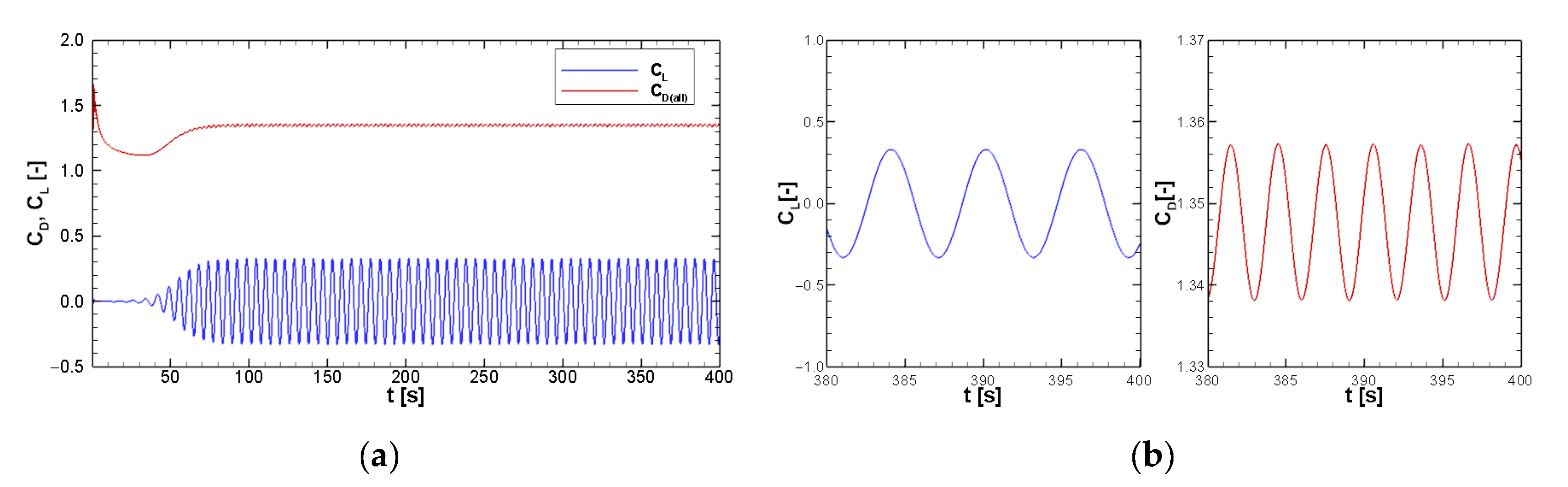
When the Reynolds number was 100, vortices were shed alternately from one side to the other, and alternating low-pressure zones were generated on the downwind side of the cylinder, giving rise to a fluctuating drag force. These widely known phenomena are clearly displayed in
Figure 12 and
Figure 13, where the vorticity magnitude and pressure with streamlines are illustrated, respectively. Periodic changes in the drag and lift forces caused by vortex shedding are also observed in
Figure 14.
The calculated drag and lift coefficients as well as the Strouhal number (
St) are summarized and compared with the results of other methods (
Table 3). It is evident that the accuracy of the proposed method is similar to those of the other methods.
3.2.2. Two Cylinders
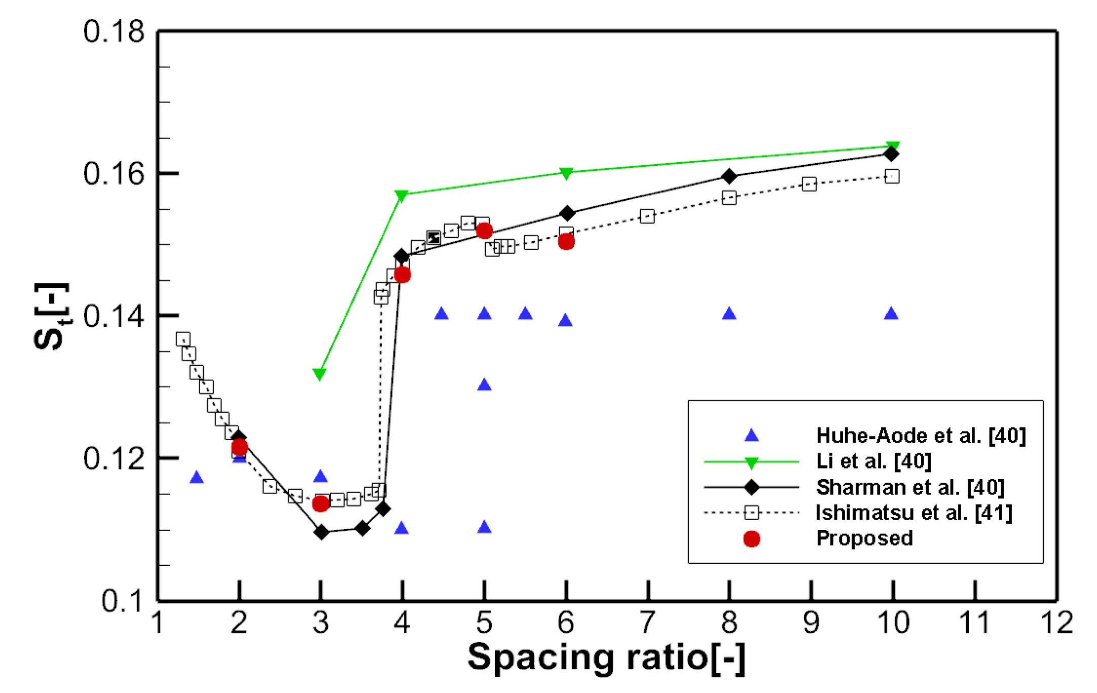
Numerical simulations of the flow around two cylinders in tandem arrangement were performed by varying the spacing ratio
from 2 to 6 at
Re = 100. Discontinuous changes in the Strouhal number and hydrodynamic forces are expected when
is approximately 4 and 5 [
40,
41].
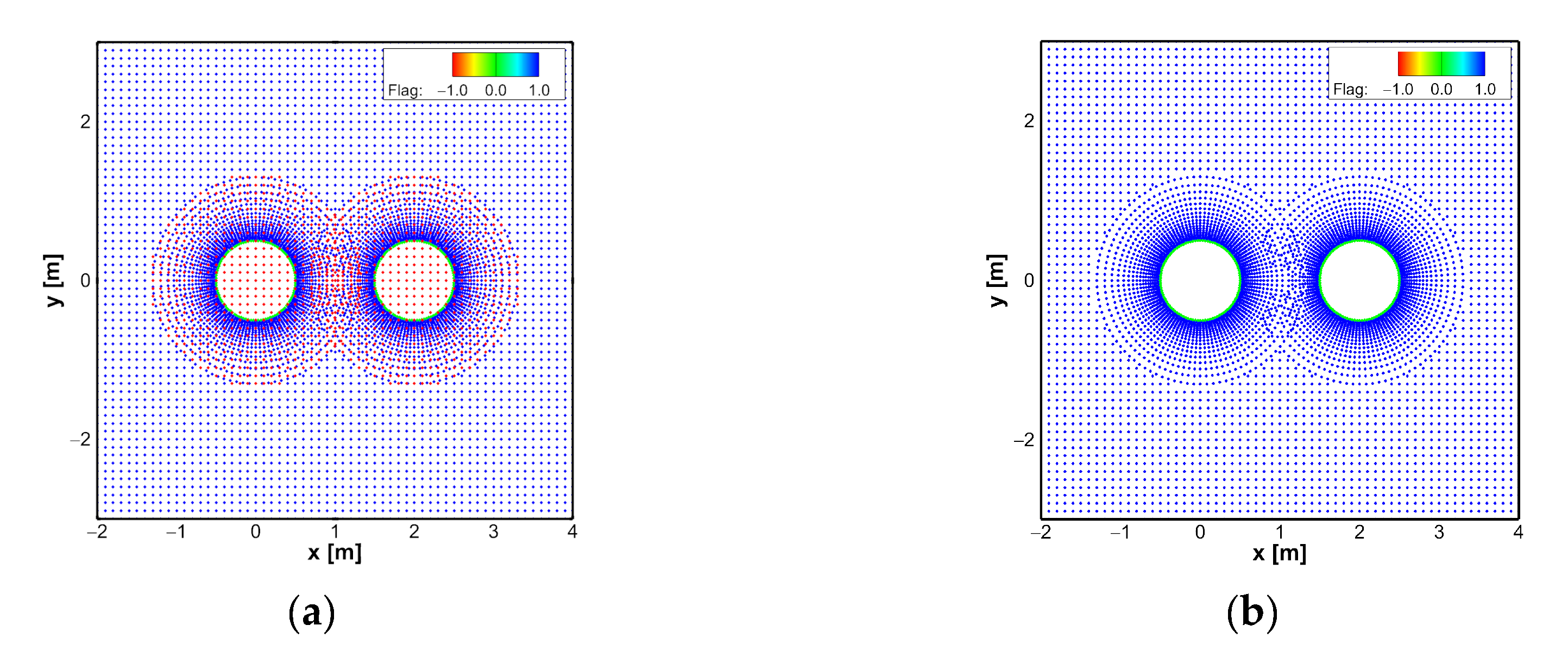
The simulation conditions were the same as those of the single cylinder, except for the number of cylinders. The distributions of the computational points near a body (a) with and (b) without inactive points at
s = 2 are exhibited in
Figure 15. It can be observed that the irregularity of the distribution increases in the region between the two cylinders. The total simulation time was 1000 s when the spacing
s was 4, but only 400 s for the other cases.
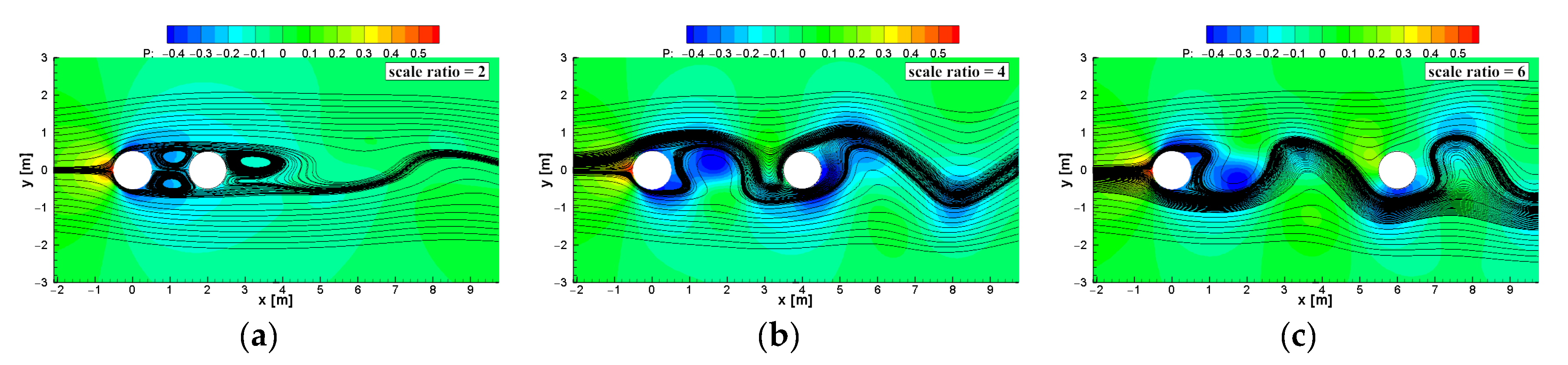
Figure 16 and
Figure 17 show the contour maps of the velocity magnitude and pressure with streamlines, respectively, for different spacing ratios
s. When
s = 2, the wake of the upstream cylinder reattaches to the downstream cylinder, forming a negative pressure that results in negative drag, as indicated in
Figure 18. The flows between the cylinders are symmetric against their centerlines, and long vortices are shed. This explains the small
St only for the downstream cylinder in
Figure 19, because the free shear layer from the upstream cylinder completely covers the downstream cylinder. When
s = 4, vortex shedding starts to occur in both the downstream and upstream cylinders. The attachment of the shear layer to the downstream cylinder is marked by an increase in the pressure coefficient at the reattachment point on the downstream cylinder surface, which causes a sudden increase in the drag coefficients of both cylinders [
33,
40]. When
s = 6, the primary vortices from the upstream cylinder do not directly reattach to the downstream cylinder, but the stretched and weakened vortices reach the downstream cylinder, which causes a decrease in the drag force acting on the downstream cylinder [
40]. The drag coefficients of both cylinders and the Strouhal numbers estimated using the proposed method are compared with the results of other methods in
Figure 18 and
Figure 19, respectively. A discontinuous change in the values is observed near the critical spacing ratio, but the overall result is in good agreement with those of the other numerical methods.


