Article

Applicability of Machine Learning for Vessel Dimension Survey with a Minimum Number of Common Points

Faculty of Navigation, Maritime University of Szczecin, 70-500 Szczecin, Poland
*
Author to whom correspondence should be addressed.
Appl. Sci. 2022, 12(7), 3453; https://doi.org/10.3390/app12073453
Submission received: 3 February 2022 / Revised: 24 March 2022 / Accepted: 26 March 2022 / Published: 29 March 2022

Abstract

:

Featured Application

Applied engineering, surveying on unstable surfaces such as docks and ships, dimensional control of floating objects, study of ship body deformations, measurements in the own (dynamic) coordinate system of objects, and coordinate transformations with low tolerance of errors.

Abstract

This paper presents the challenges encountered in the dimensional control of ships, platforms, and offshore units. This novel approach utilizes machine learning (MLP—Multilayer Perceptron Neural Network) for three-dimensional (3D) spatial coordinate transformations when only three common points are known. The proposed method was verified based on laboratory and field data. The main issue was to provide a sufficient number of valid training points. The oversampling method was used to meet this criterion. The achieved results indicate equal or better accuracy when the points were located inside the adjustment points array. In the case where the points lay outside this array, no improvement in the accuracy of the transformation was observed. The neural approach restores the transformation symmetry, and in some cases, such as the study of deformation of engineering objects, breaks the symmetry rather than restoring it.

1. Introduction

One necessary condition for training Artificial Neural Networks (ANNs) to find optimal solutions is to have a sufficiently large training dataset. Artificial neural networks are currently used to solve many technical and computational problems, including coordinate transformation. For the sake of convenience, ortho Cartesian coordinate systems are commonly used to determine the position of objects in 3D space [1]. These systems are often associated with an object or figure that is in motion in navigation, hydrography, unmanned systems, mobile laser scanning, robotics, computer games, and virtual or augmented reality [2,3,4]. To determine a position in real global reference systems, positioning based on Global Navigation Satellite Systems (GNSS) is generally used, and in some areas, traditional methods of geodetic measurements with the use of Total Station [5,6,7] are employed. Due to their high precision, Total Station instruments are widely used, for example, in engineering surveying for monitoring engineering structures, in underground measurements for tunneling, and in measurements on ships, docks, and on-water platforms and applied engineering [6,8,9]. In the case of measurements on moving platforms (airplanes, ships, and robots), the instrument-measuring sensor (laser scanner, camera, Total Station, etc.) is generally not precisely leveled, and its spatial orientation is determined by three coordinates and three Euler angles that define the rotation of the instrument about each axis of the coordinate system. The external orientation elements of a measuring instrument (sensor) can be measured with measuring devices such as a GNSS receiver, an Inertial Measurements Unit (IMU), and a Motion Reference Unit (MRU) mounted on the measuring instruments or calculated based on external reference points with a known position. In all the cases mentioned above, to calculate the position of the sensor and the points measured by it, it is necessary to use a seven-parameter conformal transformation, which consists of: translations (3D vector coordinates), rotations (three Euler angles), and the scale factor [10,11,12,13,14]. Through conformal transformations, it is possible, inter alia, to generate a cloud of measurement points obtained from several freely oriented measurement stations. as well as to compare the stability of the location of the same points at certain time intervals, e.g., when testing the deformation of engineering structures or tectonic plate movement [15,16,17,18,19]. Conformal transformation is also commonly used in computer vision, photogrammetry, and remote sensing [20,21,22,23]. Conformal transformation is also called similarity transformation or Helmert transformation and is often written as Equation (1) [24,25,26] or is solved using novel gradient methods [27,28]. At the same time, the works [23,29] show that traditional and gradient methods of solutions of the similarity transformation give very similar results in terms of accuracy of the adjustment points.
An alternative approach to the above-described methods is the use of machine learning, especially ANNs, for coordinate transformation. The use of artificial neural networks has proved their versatility in various fields. In the case of positioning and geodetic measurements, the ANNs are of increasing interest due to their enormous potential for application in many different areas of science and technology. Previous studies on the transformation of coordinates with the use of ANNs have been conducted many times, but generally, they were based on sets from several dozen points to even several hundred thousand points (in cartographic applications). However, ANNs can determine the relationship between two coordinate systems without a mathematical model, which is beneficial in its use of complex data models of coordinates [23,27,28].
In geodetic measurements, the number of common points between measurement stations is usually lower (from a few to a dozen). In offshore surveys, combining the measurement stations into one point cloud is even more difficult. Due to the space limitations determined by the structure of the measured object (ship, platform, etc.), it is difficult to locate the areas where the measurement network points can be installed to ensure their good geometry from the point of view of accuracy. A uniform distribution of many points in the space on the ship is generally impossible; hence, forced geometrical configurations of the distribution of points are used, and the number of connection points between the measurement stations is generally lower and falls within the range of 3–6. In addition, when the object is on the water, it is not possible to precisely level the Total Station, which forces the use of conformal 3D transformations to combine the measurements into a cloud of points. Measurements on unstable (movable) surfaces are applied using the measurement technology of a completely free position, without leveling the instrument, in a local and random coordinate system related to the Total Station [16,30]. The use of ANN to solve the problem of coordinate transformation in these specific conditions, due to the very small set of data that can be used to train the network (usually 3–6 common points between measurement stations), seems very difficult or impossible.
Therefore, a general question can be raised: is it possible to solve the problem of coordinate transformation using machine learning (ANN) in the case of fewer geodetic networks, with only three common points? Can it be done with better or equal accuracy in comparison to the novel (gradient) and traditionally used methods of coordinate transformation in all kinds of scenarios? In this publication, the authors put forward the thesis that it is possible, and, despite the described difficulties, they set a goal to solve the problem of using ANN for the transformation of coordinates for a minimum number of points in a satisfactory way from the point of view of accuracy. Therefore, the specific objectives are: finding and applying a simple method of densifying the number of points in less geodetic networks, verifying whether it is possible to use ANN to solve the problem of coordinate transformation for offshore purposes with the help of a point cloud generated in this way, and verification of whether the applied approach enables the achievement of equal or higher accuracy of 3D transformation in relation to novel (gradient) and traditionally used computational methods.

2. Materials and Methods

The proposed method was verified based on laboratory and field data. The laboratory data contained two types of data: reference data and reference data distorted according to a normal (Gaussian) distribution. Field data were collected during measurements of a docked vessel that was in the water. Measurements were collected by means of the Total Free Station (TFS) technology [28]. The materials and methods section presents a description of the measurements and tests using the proposed method of densification of the geodetic networks to generate a virtual point cloud for the transformation of coordinates in off-shore measurements using ANN.
This section begins with obtaining data for coordinate transformations in laboratory and field studies. Next, the step of generating a virtual point cloud for coordinate transformation is described. Then, the method of determining the size of the learning, validation, and test ANN set is defined. As a result, the methodology of using ANN for coordinate transformations is presented. The authors would like to pay special attention to the applied, atypical but very computationally simple method of generating a virtual cloud of homological points, not used thus far for coordinate transformations. The general scheme of the transformation of coordinates, broken down into the main stages, is presented in Figure 1.

2.1. Data Preparation

This section presents the method of preparing data for laboratory and field tests, which in the next stage was used to generate a virtual point cloud for coordinate transformation using machine learning (ANN).
In laboratory tests, a set of reference data (ideal) for training neural networks was prepared, along with a set of data disturbed by random errors generated according to a normal (Gaussian) distribution. Two datasets were prepared in the field trials. Total Station measurements were taken on a ship that was docked on the water. Based on the measurement data, two different sets of common points generated two different sets of points for transformation.
The research was carried out in the first phase on the basis of laboratory data. Ideal model data based on 7 points on the sphere were adopted for the calculations. Then, the set of reference points was transformed according to the relation (1), rotated by (assumed) angles, and shifted by the translation vector (Figure 2). The scale factor was adopted as 1 due to the fact that the nature of geodetic measurements with the use of a Total Station instrument does not change the scale between the individual measurement stations.
[ X Y Z ] = λ · R · [ X Y Z ] + [ X ¯ 0 Y ¯ 0 Z ¯ 0 ] ,
where:
  • [ X ,   Y ,   Z ] T —vector (point) in the original (primary) coordinate system,
  • [ X ,   Y ,   Z ] T —vector (point) in the secondary coordinate system,
  • [ X ¯ 0 ,   Y ¯ 0 ,   Z ¯ 0 ] T —translation vector,
  • λ—scale factor,
  • R—rotation matrix.
Figure 2. Reference points for generating a virtual point cloud (general view).
Applsci 12 03453 g002
The sphere was generated in the Rhino 3D program. This is a CAD program used for modeling and creating 3D objects. In this way, common points were obtained in two coordinate systems; input was designated by the authors as local frame (LF), and output was labeled as vessel frame (VF). There can be more than one LF, which must be combined with a VF. A virtual point cloud was generated in two coordinate systems (input and output) according to the algorithm described in Section 2.2. In the second step, an additional set of data was prepared, to which random disturbances generated according to a normal (Gaussian) distribution were added.
Experimental field tests were carried out on the vessel Navigator XXI, which was in the dock, on the water. Measurements were taken with the use of a Total Station (Trimble SX10), without its leveling, in the technology of Total Free Station (TFS). Measurements on the ship were made from two measurement stations in random local coordinate systems related to the Total Station. An observation plate with a magnet feature was used for common points (Figure 3). Measurements were made in windless weather.
As a result of the measurements, a set of measurement data was created. The base points altogether between the stations were used to generate a virtual point cloud.

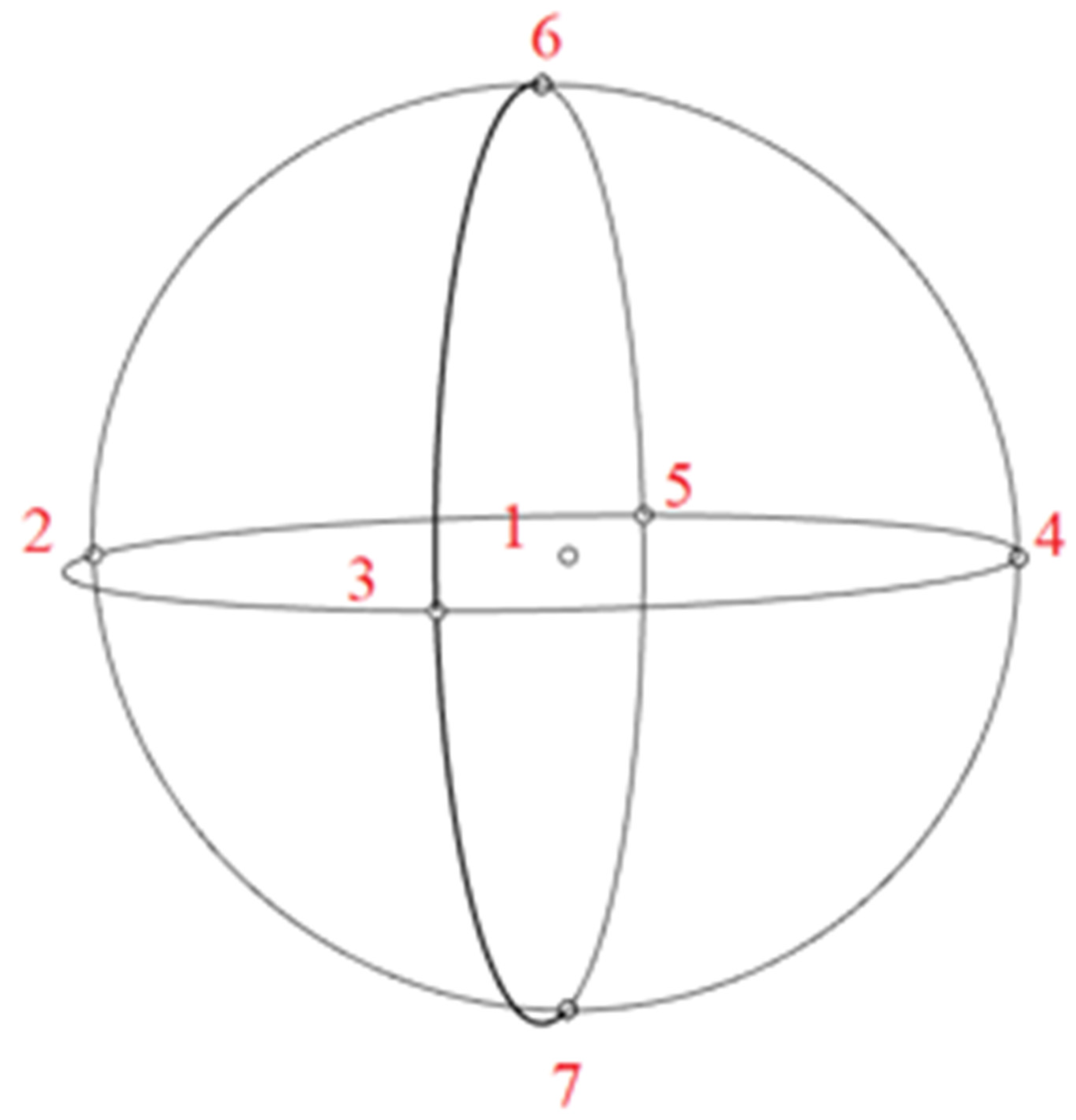
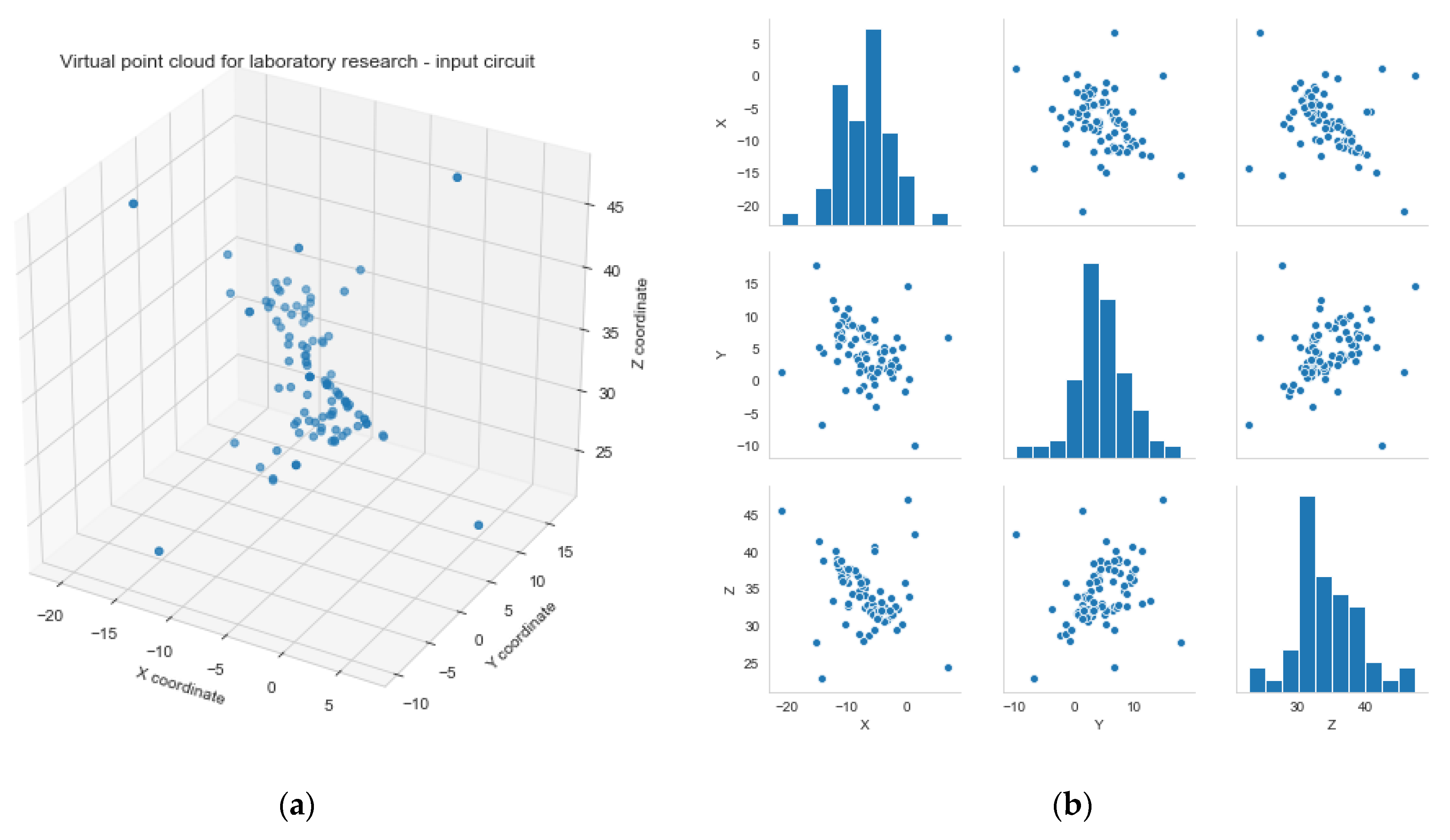
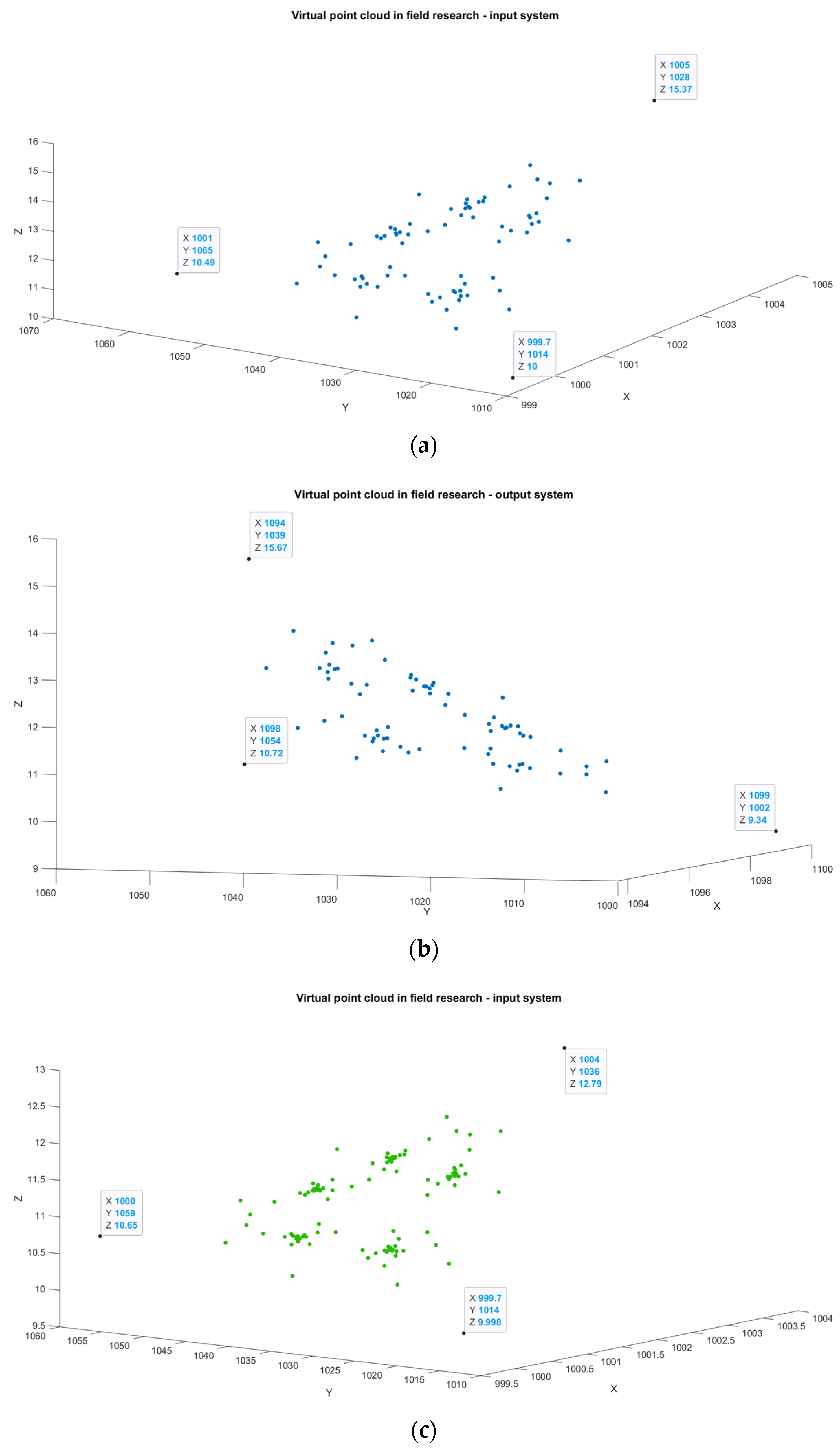
2.2. Generation of a Virtual Point Cloud

This section describes how to generate the virtual point cloud used to train the ANN to solve the problem of coordinate transformation in some reference frames. The scheme of generating a virtual point cloud is shown in Figure 4.
The virtual point cloud was generated on the basis of base points (homologous in two coordinate systems). First, on the basis of the base points (blue in Figure 4) and the geometric center (centroid) of these points (purple in Figure 4), further points are generated (green in Figure 4). The geometric center (centroid) of the base points is calculated as the arithmetic mean of the individual coordinates x , y , and z (2). Centroid corresponds to the center of geometry (centroid) for an isolated system and unit masses. Then, each of the three points, consisting of at least one point newly generated in the previous step, is used to generate additional points. This operation is repeated until the assumed number of virtual points is reached. Generating virtual point clouds was conducted with the application of the Matlab Software. The method of determining the number of required points is described in Section 2.3: The use of artificial neural networks.
X C = i = 1 N ( X i ) 3 ,     Y C = i = 1 N ( Y i ) 3 ,     Z C = i = 1 N ( Z i ) 3 ,
where:
  • X C ,   Y C , Z C —coordinates of the centroid (center of mass)
The applied idea of generating a virtual point cloud is computationally very simple, where the arithmetic mean is used many times. This approach is based on the symmetry of transformations with respect to the displacement. In symmetrical transformations, the angles (symmetry with respect to rotation, shift by angle) and distances (symmetry with respect to the shift translation, time is omitted) are preserved. These symmetries are characteristic of orthogonal transformations, where the invariant of the transformation is the vector length (in real spaces). Therefore, the distances between the points are maintained (for a scale equal to 1) [31,32,33]. Such an assumption was made in the discussed case, and it was used to generate virtual points homologous to machine learning (ANN) to solve the problem of coordinate transformation in some reference frames.

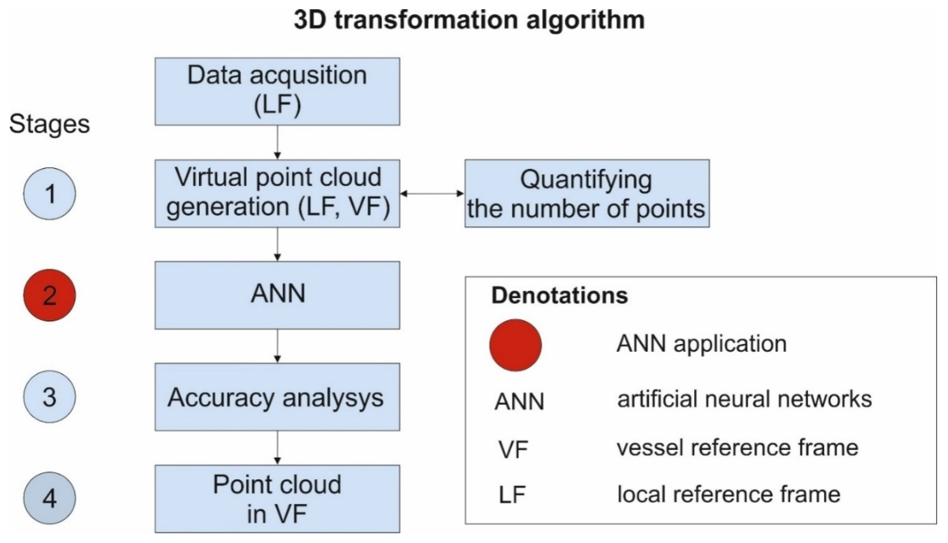
2.3. The Use of Artificial Neural Networks

For effective training of neural networks, more training cases are needed, producing more connections in the network. One of the ways to determine the proportion of the number of training cases to the total number of network parameters constructed during training is the coefficient ρ (3) proposed in the work [34]:
ρ = U ( I 1 ) · H + ( H + 1 ) · O ,
where:
  • U—the number of learning cases
  • I—the number of neurons in the input layer
  • H—the number of neurons in the hidden layer
  • O—the number of neurons in the output layer
For the proper operation of the network, the factor ρ should be between 1.8 and 2.2. On the basis of preliminary studies, MLP 3-k-3 networks were obtained, where the number of neurons in the hidden layer k was usually between 6 and 10 neurons (according to Equation (3)). Therefore, the number of learning cases, according to Equation (3), was determined to be at least 60. The SANN (Statistica Automatic Neural Networks) module of the STATISTICA software was used for the construction and analysis of neural networks. The input vector comprised the coordinates of the generated points before the transformation, and the output vector comprised the coordinates of the generated points after the transformation. Usually, the learning set does not exceed 80% of the data and the rest is used to test the solutions found [34]. In this publication, three subsets were created from the dataset: the training sample constituting 70% of the total data, the validation sample (15%), and the test sample (15%). Both MLP and RBF networks were checked in the automatic network wizard. In regression problems, such as the problem under discussion, the sum of squares of differences was used as a function of the error. As activation functions, both in the hidden layer and in the output layer, the following functions were tested: linear, logistic, hyperbolic tangent, and exponential. SANN has several options for training MLP networks: the BFGS error back propagation algorithm (Broyden–Fletcher–Goldfarb–Shanno), the Scaled Conjugate Gradient algorithm, and the fastest descent algorithm. In the case of an RBF network with linear activation functions, the learning process takes place in two stages. The first arranges radial functions using only the input variables from the data. In the second stage, the weights connecting the radial functions with the output neurons are determined. With the configured settings, the automatic SANN wizard checked 100 networks, both MLP and RBF types, from which the top 5 were selected. The highest correlation statistics for the test and validation sample were adopted as the criterion for selecting the best networks.

3. Results

Generating a Virtual Point Cloud

Laboratory tests were carried out on the basis of ideal data distributed over the sphere. There were six points distributed on the sphere, and an additional seventh point was the center of the sphere. Then, on their basis, a set of 98 points was generated, and it was assumed that this set would be the input system for the transformation.
Then, the sphere with the set of seven base points was shifted by any (random) vector and turned by any (random) angle. Similarly to the first case, a second virtual point cloud was created on the basis of the base points. This set was called the output system. Points were generated according to the algorithm described in Section 2.2. Table 1 presents the thus-obtained coordinates of selected homologous points of virtual point clouds in the input and output systems.
The distribution of the points generated in this way is shown in Figure 5. As can be seen from the data presented in Table 1 and in Figure 5, the points that are artificially generated are located in the central part of the sphere where their concentration is greatest. The graph shows the relationships in each dataset. The diagonal plots show the marginal distribution of the data in each column. The border points, which were the basis for generating a virtual point cloud, also come to the fore, where the concentration of virtual points is the lowest. After generating virtual point clouds, the distances between the individual points in each of the input and output systems were verified. The calculated distances were identical, which confirmed the preservation of symmetry with respect to translation and rotation, as well as the invariability of the scale, and therefore the homology of points in the input and output systems.
The dataset included the coordinates of 105 points in the input and output frames. The networks were learned on a set of 73 points, which included 7 basis points. The test set included 16 points, and a validation set 16 points. The points were randomly selected in addition to the 7 base points. In the STATISTICA Neural Networks (SANN) package, the top 5 were selected out of 100 learned and analyzed networks, which turned out to be MLP networks with one hidden layer with a number of neurons from 4 to 10. For the hidden and output layers, all networks had a linear activation function. The maximum error of the selected networks did not exceed the value of 1 · 10 7 in the validation and test set for the input data adopted with a precision of writing of 1 · 10 3 and conventionally expressed in meters.
The comparison of the output values with the values determined by the network team gave the “average error of fit” at the level of 3 · 10 5 m for the variable x , 6 · 10 6 m for the variable y , and 3 · 10 6 m for the variable z . Moreover, for the seven base points, the differences in the coordinates between the input system and the results obtained from the analytical model (1) and the neural networks were compared (Figure 6, Table 2).
By statistically comparing the differences in coordinates between the output system and the results obtained from the analytical model and neural networks, statistically, significant differences were found. These are particularly visible in the case of the absolute values of differences. The test results confirm the better accuracy of the network; for the x and y variables, there is a significant statistical difference, and for the z variable, although the results are slightly worse, it is not a statistically significant difference.
The conducted laboratory tests confirmed the correctness of the proposed method. In each case, the ANNs achieved higher accuracies than the similarity transformation algorithm. Therefore, field research was initiated.
The field research was carried out on two datasets derived directly from the measurements; the set marked as Z1 contained 87 points, and the set marked as Z2 contained 141 points.
Datasets based on measurement data were obtained from measurements on the Navigator XXI vessel. Two measuring stations were used. In the case of the Z1 set, three points were assumed, which were measured in one measurement series. Then, an artificial point cloud was generated from the points, and the final set consisted of 87 points. The second set of data was also based on measurement data obtained from measurements on the Navigator XXI vessel. The same measurement stations were used in this case, while other points of the measurement network were adopted. In the case of this set, three points were assumed, which were measured in several series of measurements, which should indicate that the coordinates will be obtained with better accuracy. Then, an artificial point cloud was generated from the three points, and the final set consisted of 141 points. The summary of the data for both measuring stations for the Z1 and Z2 sets is shown in Table 3 and Figure 7.
The dataset Z1 included three points, on the basis of which a set of 87 points was generated in the input and output coordinate systems. The input data were the coordinates of the points obtained on the measuring station No. 2 (LF system), while the output data were the coordinates of the points obtained on the measuring station No. 1 (VF system). The networks were learned on a set of 61 points that contained 3 basis points. The test set included 13 points, and a validation set 13 points. The points were randomly selected, except for the 3 base points. For the Z1 set, the top five networks were selected, which turned out to be MLP networks with one hidden layer with the number of neurons from 6 to 10. For the hidden layer, two of these networks had linear activation functions, two had a logistic function, and one had an exponential function. For the output layer, all networks had a linear activation function. The maximum error of the selected networks did not exceed the value of 3 · 10 5 in the validation and test set.
The dataset Z2 included three points, on the basis of which a set of 141 points was generated in the input and output coordinate systems. The input data were the coordinates of the points obtained on the measuring station No. 2 (LF system), while the output data were the coordinates of the points obtained on the measuring station No. 1 (VF system). The networks were learned on a set of 99 points, which included 3 basis points. The test set included 21 points, and the validation set 21 points. The points were randomly selected, except for the 3 base points. For the Z2 set, the top five networks were selected, which turned out to be MLP networks with one hidden layer with the number of neurons from 4 to 9. For the hidden layer, two of these networks had linear activation functions, one logistic function, one tanh function, and one exponential. For the output layer, all networks had a linear activation function. The maximum error of the selected networks did not exceed the value of 4 · 10 6 in the validation and test sets.
The results for both sets are about two orders more accurate than the precision of the Total Free Station (TFS) and TLS (Terrestrial Laser Scanner—Figure 8) measurements, which, from a practical point of view, does not burden the measurements with errors and is negligible. With transformation errors at this level, we can consider them insignificant. From the point of view of the precision of the measurement of TFS and TLS (1–3 · 10 3 m), these values are infinitesimal and the coordinate transformations, with errors two orders less than the accuracy of the coordinates, can be treated as approximately error-free.

4. Discussion

The study results are summarized in Table 4.
Based on the data presented in Table 4, it can be concluded that, in each analyzed case, both for laboratory and field data, the best results were obtained by MLP networks. The number of selected networks was five, and the number of hidden layers was one. The number of neurons did not exceed 10. In all analyzed cases, the optimal function turned out to be the linear activation function for the output layer, while for the hidden layer, the activation functions were different, with the predominance of linear ones. The maximum error of the selected networks did not exceed the value of 3 · 10 5 m in the validation and test set for the input data adopted with the precision of 1 · 10 3 m and expressed conventionally in meters, which should be considered a very good result. In the case of an average match error, the result is not that good. For laboratory data, ANNs have an advantage over the conformal transformation, being more precise. For the field data, in the case of the Z1 set, ANNs are slightly more accurate than Total Station (1 · 10 3 m) and Terrestrial Laser Scanning (1 3 · 10 3 m), while in the case of the Z2 sets, the transformation by similarity turned out to be more accurate (due to the greater error of the Z coordinate for ANN). However, these results for this dataset are still an order more accurate than the precision of the input data obtained by Terrestrial Laser Scanning, which should also be considered satisfactory. In the areas between the base points (validation and test data)—inside the transformation area—ANN has a decisive advantage, while in the case of common points in the case of field data, the errors in both the traditional and the proposed algorithms are at the same level. At the same time, the base point errors for the laboratory dataset are still reduced for ANN. It should therefore be summarized that machine learning (ANNs) with the applied method on the common points (baseline) obtains RMSEs of the same level in the case of field data, and better in the case of laboratory data for the minimum number of common points. At the same time, for the areas inside the base points (the area inside the transformation), ANNs give reduced errors in each case.
In addition, it can be seen that different activation functions are found for the field data and the different sets of base points used for the transformation. The conclusion is that ANN transformations are on the same level of accuracy or even better suited to conformal transformations for the specific cases they concern (for minimum number of common points), but cannot be directly replicated for other sets of points. The uniqueness provides a better match between the input and output data, which is an advantage of ANN, but changing the dataset means that these functions should be searched anew, which in turn can be considered as a disadvantage (one case cannot be directly transposed into another). Comparing the average match error (Table 2), it can be observed that the obtained results from the transformation of the X, Y, Z coordinates using the analytical method and the ANN are slightly different. The difference that is shown in the diagrams below is in favor of using the ANN (Figure 9).

5. Conclusions

This paper proves that machine learning can be applied for coordinate transformations, even when the dataset for training the network consists of only a few (even minimum) points. The paper provides guidance on how to solve this problem and oversample a virtual point cloud for network training. The authors also found appropriate networks that provide better or the same level of accuracy compared to the novel (gradient) and traditionally used conformal transformations in applied scenarios. However, when the scenario is extended beyond the area of the points used for ANN learning (e.g., in the case of extrapolation), no increased accuracy of the results is expected. Therefore, the proposed method can be applied to points that are inside the adjustment points, and only in this case achieve equal or slightly better accuracy for the coordinate transformation.
This raises the question of whether the use of conformal transformations for lower-scale coordinate systems, especially with the minimum number of common points, makes sense, since it can be carried out using ANN and more precisely at the same time, but in limited scenarios (inside adjusted points). Can such a transformation be justified in every situation? It should be noted that the ANN transformation is “tailor-made” and somehow restores the transformation symmetry, and in some cases, such as the study of the deformation of engineering objects, breaks the symmetry rather than restoring it, because this is how we can determine which points have moved and which have not. The proposed method of transformation can be considered closer to symmetry-back transformations. The benefit of its use is when we do not have additional common points to solve the transformation with mean square errors, especially when the measurement system is not a rigid system, e.g., it is exposed to the deformations due to thermal weather conditions. This can be considered in the measurement of floating objects; hence, the method may find application in the offshore industry and, in the authors opinion, is of great potential for applied engineering. The authors intend to focus further research on the potential applications of this transformation method for positioning moving objects on the water in inland navigation, using a non-metric industrial camera as a data source.

Author Contributions

I.G., A.T., G.S. and L.K. proposed the original idea for this study; A.T., W.Ś. and G.S. implemented the experiments for off-shore purposes; I.G., G.S., L.K., A.T. and T.K. wrote the paper, with revisions by W.Ś. and T.K. All authors have read and agreed to the published version of the manuscript.

Funding

This research was funded by the grant 3/SKG/20, financed from a subsidy of the Ministry of Science and Higher Education for statutory activities.

Institutional Review Board Statement

Not applicable.

Informed Consent Statement

Not applicable.

Data Availability Statement

The data used to support the findings of this study are available from the corresponding author upon request.

Acknowledgments

The authors would especially like to thank Krzysztof Beczkowski and Tomasz Ziębka for their involvement in the data acquisition.

Conflicts of Interest

The authors declare no conflict of interest.

References

  1. Hooijberg, M. Practical Geodesy; Springer: Jersey City, NJ, USA, 1997. [Google Scholar] [CrossRef]
  2. Titterton, D.; Weston, J. Strapdown Inertial Navigation Technology, 2nd ed.; The American Institute of Aeronautics and Astronautics: Herts, UK; The Institution of Electrical Engineers: Reston, VA, USA, 2004. [Google Scholar]
  3. Krichenbauer, M.; Yamamoto, G.; Taketom, T.; Sandor, C.; Kato, H. Augmented Reality versus Virtual Reality for 3D Object Manipulation. IEEE Trans. Vis. Comput. Graph. 2018, 24, 1038–1048. [Google Scholar] [CrossRef] [PubMed]
  4. Sra, M.; Garrido-Jurado, S.; Schmandt, C.; Maes, P. Procedurally generated virtual reality from 3D reconstructed physical space. In Proceedings of the ACM Symposium on Virtual Reality Software and Technology VRST, Munich, Germany, 2–4 November 2016; pp. 191–200. [Google Scholar] [CrossRef] [Green Version]
  5. Hofmann-Wellenhof, B.; Lichtenegger, H.; Wasle, E. GNSS—Global Navigation Satellite Systems—GPS, GLONASS, Galileo, and More; Springer: Vienna, Austria, 2007. [Google Scholar] [CrossRef] [Green Version]
  6. Schofield, W.; Breach, M. Engineering Surveying, 6th ed.; Butterworth-Heinemann: Oxford, UK, 2007. [Google Scholar]
  7. Soler, T. A compendium of transformation formulas useful in GPS work. J. Geod. 1998, 72, 482–491. [Google Scholar] [CrossRef] [Green Version]
  8. Kilford, W.K. Surveying for engineers. Surv. Rev. 1979, 25, 94–96. [Google Scholar] [CrossRef]
  9. National Occupational Standards Offshore Surveying and Positioning; Taylor & Francis Online: Abingdon, UK, 2013; Available online: https://taylorandfrancis.com/ (accessed on 2 February 2022).
  10. Baetslé, P.-L. Conformal transformations in three dimensions. Photogramm. Eng. Remote Sens. 1966, 35, 816–824. [Google Scholar]
  11. Ruffhead, C. Equivalence properties of 3D conformal transformations and their application to reverse transformations. Surv. Rev. 2020, 53, 158–168. [Google Scholar] [CrossRef]
  12. Deakin, R.E. 3-D coordinate transformations. Surv. Land Inf. Syst. 1998, 58, 223–234. [Google Scholar] [CrossRef]
  13. Schut, G.H. Similarity Transformation and least Squares. Photogramm. Eng. 1973, 621–627. [Google Scholar]
  14. Markley, F.L.; Crassidis, J.L.; Markley, F.L.; Crassidis, J.L. Euler Angles. In Fundamentals of Spacecraft Attitude Determination and Control; Springer: New York, NY, USA, 2014. [Google Scholar] [CrossRef]
  15. Brazeal, R. Three Dimensional Coordinate Transformations for Registering Terrestrial Laser Scanning Datasets Based on Tie Points. No. SUR 6905-Point Cloud Analysis. 2013. Available online: https://www.researchgate.net/publication/265014559_THREE_DIMENSIONAL_COORDINATE_TRANSFORMATIONS_FOR_REGISTERING_TERRESTRIAL_LASER_SCANNING_DATASETS_BASED_ON_TIE_POINTS?channel=doi&linkId=53fbef070cf2dca8fffee54b&showFulltext=true (accessed on 2 February 2022).
  16. Stępień, G.; Tomczak, A.; Loosaar, M.; Ziębka, T. Dimensioning method of floating offshore objects by means of quasi-similarity transformation with reduced tolerance errors. Sensors 2020, 20, 6497. [Google Scholar] [CrossRef] [PubMed]
  17. El-Ashmawy, K.L.A. A comparison between analytical aerial photogrammetry, laser scanning, total station and global positioning system surveys for generation of digital terrain model. Geocarto Int. 2014, 154–162. [Google Scholar] [CrossRef]
  18. Huang, J.; You, S. Point cloud matching based on 3D self-similarity. In Proceedings of the 2012 IEEE Computer Society Conference on Computer Vision and Pattern Recognition Workshops, Providence, RI, USA, 16–21 June 2012; pp. 41–48. [Google Scholar] [CrossRef]
  19. Bejger, A.; Gawdzińska, K. An attempt to use the coherence function for testing the structure of saturated composite castings. Metalurgija 2015, 54, 361–364. [Google Scholar]
  20. Brazetti, L.; Scaioni, M. Automatic orientation of image sequences for 3D object reconstruction: First results of a method integrating photogrammetric and computer vision algorithms. Int. Arch. Photogramm. Remote Sens. 2009, XXXVIII, 25–28. [Google Scholar]
  21. Colomina, I.; Molina, P. Unmanned aerial systems for photogrammetry and remote sensing: A review. ISPRS J. Photogramm. Remote Sens. 2014, 92, 79–97. [Google Scholar] [CrossRef] [Green Version]
  22. Sweeney, C.; Kneip, L.; Höllerer, T.; Turk, M. Computing similarity transformations from only image correspondences. In Proceedings of the IEEE Conference on Computer Vision and Pattern Recognition, Boston, MA, USA, 7–12 June 2015; pp. 3305–3313. [Google Scholar] [CrossRef] [Green Version]
  23. Śledziowski, J.; Terefenko, P.; Giza, A.; Forczmański, P.; Łysko, A.; Maćków, W.; Stępień, G.; Tomczak, A.; Kurylczyk, A. Application of Unmanned Aerial Vehicles and Image Processing Techniques in Monitoring Underwater Coastal Protection Measures. Remote Sens. 2022, 14, 458. [Google Scholar] [CrossRef]
  24. Jue, X. Research on close-range photogrammetry with big rotation angle. Int. Arch. Photogramm. Remote Sens. Spat. Inf. Sci. 2008, XXXVII, 11–14. [Google Scholar]
  25. Lin, D. An Information-Theoretic Definition of Similarity. 1998. Available online: https://www.cse.iitb.ac.in/~cs626-449/Papers/WordSimilarity/3.pdf (accessed on 2 February 2022).
  26. Henderson, D. Euler Angles, Quaternions, and Transformation Matrices. NASA JSC Report; 1977; pp. 1–39. Available online: https://ntrs.nasa.gov/search.jsp?R=19770019231 (accessed on 2 February 2022).
  27. Odziemczyk, W. Application of simulated annealing algorithm for 3D coordinate transformation problem solution. Open Geosci. 2020, 12, 491–502. [Google Scholar] [CrossRef]
  28. Stępień, G.; Zalas, E.; Ziębka, T. New approach to isometric transformations in oblique local coordinate systems of reference. Geod. Cartogr. 2017, 66, 291–303. [Google Scholar] [CrossRef]
  29. Stępień, G. Transformacje Symetryczne w Nachylonych Układach Odniesienia z Wykorzystaniem Metod Analizy Funkcjonalnej; Wydawnictwo Naukowe Akademii Morskiej w Szczecinie: Szczecin, Poland, 2018. [Google Scholar]
  30. Denton, A. Marine surveying of offshore units. In Offshore Surveying for the Civil Engineering Industry; Institution of Civil Engineers: London, UK, 1977; pp. 1–8. [Google Scholar] [CrossRef]
  31. Brading, K.; Castellani, E.; Teh, N. Symmetry and Symmetry Breaking. Stanford Encyclopedia of Philosophy. 2013. Available online: https://plato.stanford.edu/entries/symmetry-breaking/ (accessed on 12 December 2018).
  32. Castillo, G.F.T. Point symmetries of the Euler—Lagrange equations. Rev. Mex. Fıs. 2014, 60, 129–135. [Google Scholar]
  33. Andrea, T.A.; Kalayeh, H. Applicatios of neural networks in quantitative structure-activity relationships of dihydrofolate reductase inhibitors. J. Med. Chem. 1991, 34, 2824–2836. [Google Scholar] [CrossRef] [PubMed]
  34. Géron, Hands-on Machine Learning with Scikit-Learn, Keras, and TensorFlow: Concepts, Tools, and Techniques to Build Intelligent Systems; O’Reilly Media, Inc.: Sebastopol, CA, USA, 2019.
Figure 1. Coordinate transformation algorithm for offshore purposes using ANN.
Applsci 12 03453 g001
Figure 3. Total Free Station (TFS) measurements in a dock on the water, (a) total station on the floating dock, (b) vessel Nawigator XXI–measured object.
Applsci 12 03453 g003
Figure 4. Generating a virtual point cloud, x1–x3–base points, y1–centroid, z1–z3–mean of the coordinates: x, y and z.
Applsci 12 03453 g004
Figure 5. Virtual point cloud for laboratory research. Input coordinate system—(a) points distribution, (b) coordinates correlation diagram; output coordinate system—(c) points distribution, (d) coordinates correlation diagram.
Applsci 12 03453 g005aApplsci 12 03453 g005b
Figure 6. Analysis of differences in analytical and ANN results: (a) for X coordinates, (b) for Y coordinates, (c) for Z.
Applsci 12 03453 g006aApplsci 12 03453 g006b
Figure 7. A virtual point cloud in field research for two measurement stations—Z1 dataset in blue color: (a) input coordinate system, (b) output coordinate system, Z2 in green color (c) input coordinate system, (d) output coordinate system.
Applsci 12 03453 g007aApplsci 12 03453 g007b
Figure 8. Terrestrial Laser Scanning (TLS) point cloud of Navigator XXI vessel for field research validation.
Applsci 12 03453 g008
Figure 9. Comparing the results from the analytical (a) and network (b) model. Denotations xm-xp—errors for analytic (1) model, xs-xp—errors for the ANN.
Applsci 12 03453 g009
Table 1. Virtual point cloud in laboratory tests (selected points).
The Input Layout [m]The Output System [m]
NrXYZXYZ
1−7.00004.000035.0000−1.800026.400052.5000
21.2507−9.842242.302113.454517.463753.1658
36.90826.700624.40445.664038.343441.7928
4−15.250717.842227.6979−17.054535.336351.8342
5−20.90831.299445.5956−9.264014.456663.2072
60.1754314.681847.14133.158835.913066.5682
7−14.1754−6.681822.8587−6.758816.887038.4318
81.25067−9.842242.302113.454517.463753.1658
90.38630.286133.90225.772827.402349.1529
10−2.36394.900231.46810.688030.381148.9309
105−2.45401.562631.59332.120527.557947.8630
Table 2. Transformation of coordinates of a virtual point cloud.
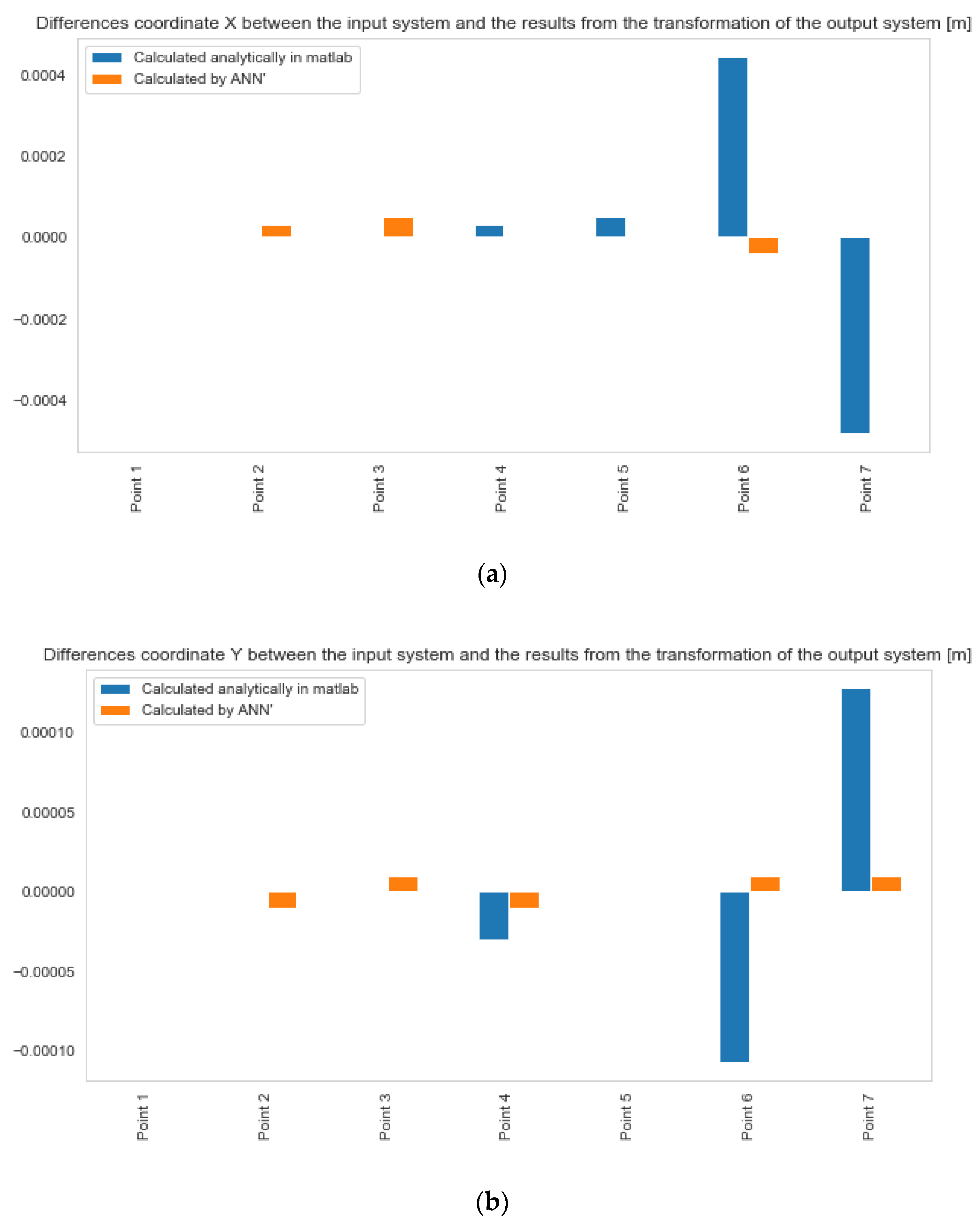
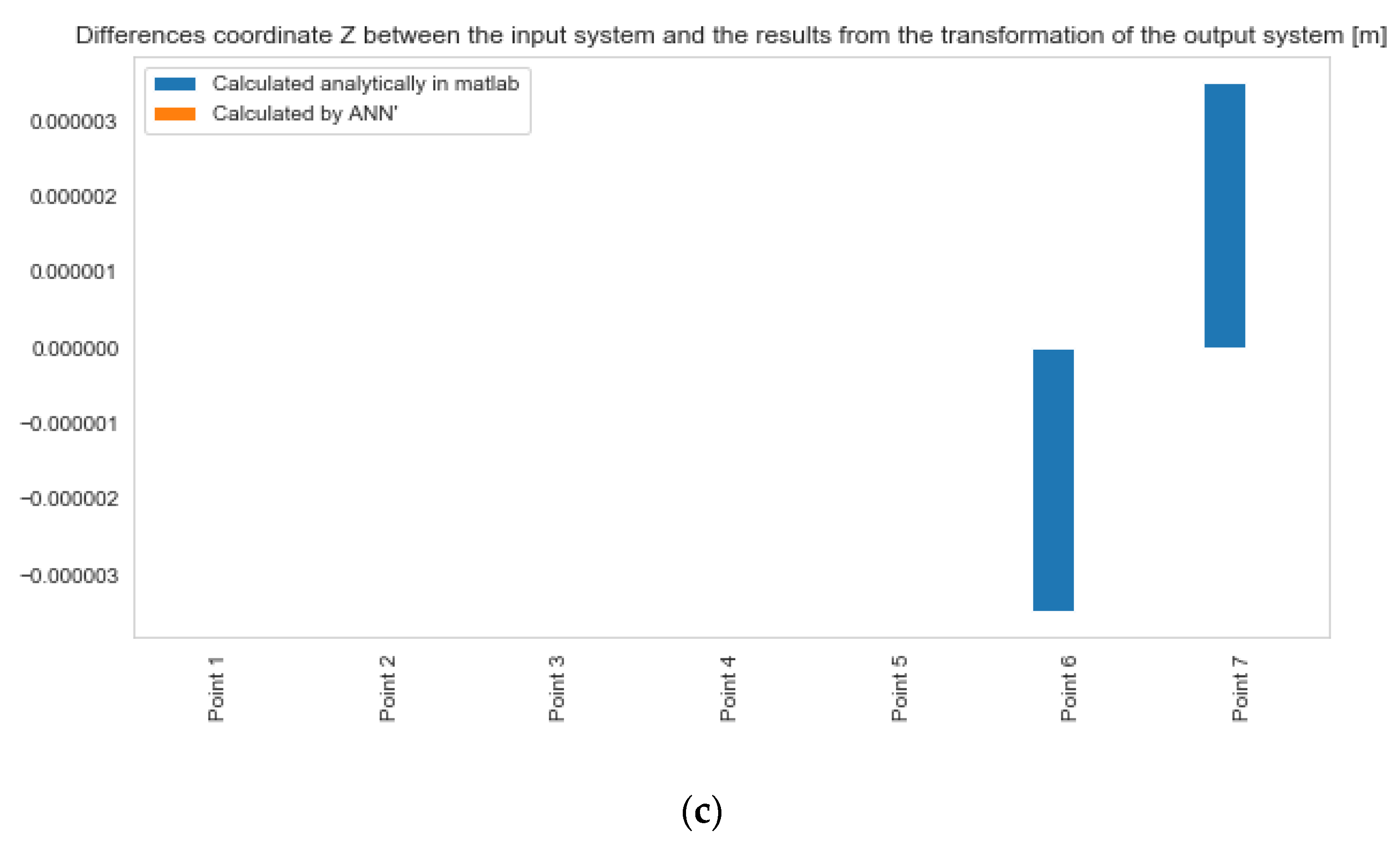
Coordinate Differences between the Input System and the Results from the Transformation of the Output System [m]
Calculated Analytically in MatlabCalculated by ANN
XYZXYZ
RMSE 2 · 10 4 6 · 10 5 2 · 10 6 3 · 10 5 6 · 10 6 3 · 10 6
RMSE
(of point)
2.6 · 10 4 3.1 · 10 5
Table 3. A virtual point cloud in field research, datasets Z1 and Z2.
Station 1—Input Coordinate System for Set Z1Station 2—Output Coordinate System for Set Z1 Station 1—Input Coordinate System for Set Z2Station 2—Output Coordinate System for Set Z2
NrXYZXYZNrXYZXYZ
11003.0071035.29013.3071095.8101031.87013.29911002.1911038.65511.8201096.7671028.60811.674
21002.4131037.86512.6201096.5211029.35512.50721001.6631039.58911.4981097.3361027.71511.308
31002.6281038.65412.8431096.3521028.54912.70531001.8321040.69411.6151097.2261026.59911.388
41002.6831037.27012.9231096.2281029.92512.83741001.8951039.64611.6441097.1091027.64111.457
51002.6941045.24312.8191096.6251021.97112.44351001.7971039.97611.5861097.2241027.31811.384
61003.1881032.78513.5421095.5051034.35313.62861001.8421040.10511.6151097.1861027.18611.410
71002.2151038.72412.3911096.7591028.51712.24371001.8461039.90911.6151097.1731027.38211.417
81002.6991038.91712.9171096.2961028.28012.77281001.8061046.35911.6551097.5451020.94511.221
91002.7011036.80812.9501096.1871030.38312.88191002.3741036.92811.9181096.4981030.31811.838
85999.6861013.5769.9981097.9361053.83210.717139999.6861013.5769.9981097.9361053.83210.717
861000.8311065.35710.4861099.4731002.0769.3441401000.0001059.38410.6481099.9981008.0769.707
871004.7891027.56515.3681093.6761039.41415.6741411003.7761035.85612.7891095.0611031.28412.774
Table 4. Parameters of the ANNs used for laboratory and field data.
ParameterLaboratory Tests Field Research
Master Data (Ideal)Data DistortedDataset Z1Dataset Z2
Type of networkMLPMLPMLPMLP
No. of chosen networks5555
No. of hidden layers1111
No. of neurons4–104–106–104–9
Activation function for the hidden layerlinearlinearLinear—2
Logistics—2
Exponential—1
Linear—2
Logistics—1
Tanh—1
Exponential—1
Activation function for the output layerlinearlinearlinearlinear
Number of points (total)10510587141
Training set (no. of points) 75756199
Validation set15151321
Test set15151321
Maximum error [mm] in the validation and test set 1 · 10 4 1 · 10 4 3 · 10 2 4 · 10 3
Mean error mp [mm] of the ANN
and analytical (similarity and gradient) model
3 · 10 2 1 · 10 1 1.09 3.84
1 · 10 1 1 · 10 1 1.11 1.91
Publisher’s Note: MDPI stays neutral with regard to jurisdictional claims in published maps and institutional affiliations.

