Article

Prediction Model for the Performance of Different PV Modules Using Artificial Neural Networks

1
Solar Energy Research Institute, Universiti Kebangsaan Malaysia, Bangi 43600, Selangor, Malaysia
2
Faculty of Science and Natural Resources, Universiti Malaysia Sabah, Kota Kinabalu 88400, Sabah, Malaysia
*
Authors to whom correspondence should be addressed.
Appl. Sci. 2022, 12(7), 3349; https://doi.org/10.3390/app12073349
Submission received: 8 March 2022 / Revised: 21 March 2022 / Accepted: 24 March 2022 / Published: 25 March 2022

Abstract

:
This study presents a prediction model for comparing the performance of six different photovoltaic (PV) modules using artificial neural networks (ANNs), with simple inputs for the model. Cell temperature (Tc), irradiance, fill factor (FF), short circuit current (Isc), open-circuit voltage (Voc), maximum power (Pm), and the product of Voc and Isc are the inputs of the neural networks’ processes. A Prova 1011 solar system analyzer was used to extract the datasets of IV curves for six different PV modules under test conditions. As for the result, the highest FF was the mono-crystalline with an average of 0.737, while the lowest was the CIGS module with an average of 0.66. As for efficiency, the most efficient was the mono-crystalline module with an average of 10.32%, while the least was the thin-film module with an average of 7.65%. It is noted that the thin-film and flexible mono-modules have similar performances. The results from the proposed model give a clear idea about the best and worst performances of the PV modules under test conditions. Comparing the prediction process with the real dataset for the PV modules, the prediction accuracy for the model has a mean absolute percentage error (MAPE) of 0.874%, with an average root mean square error (RMSE) and mean absolute deviation (MAD) of, respectively, 0.0638 A and 0.237 A. The accuracy of the proposed model proved its efficiency for predicting the performance of the six PV modules.

1. Introduction

Solar energy has become one of the world’s most essential resources in the last decade, leading to the development of photovoltaic (PV) cells. The photovoltaic (PV) system contains many components such as cells, wires, inverters, structures, and mechanical connections. The output power from this system is measured by the peak kilowatt, which indicates the amount of electrical power delivered when the sun is at its highest point [1]. With the number of advantages of the PV system, many different applications have started to depend on it, such as solar systems in homes, pumps, PV and thermal collector systems, and building-integrated photovoltaic (BIPV) systems [2,3,4,5,6]. PV performance is influenced by environmental factors such as wind, temperature, dust pollution, and installation factors such as the tilt angle and area [1,7,8]. Many previous studies have focused on the result of dust on PV systems. The position of PV cells, the type of PV cells, the type of dust product (ash, carbon, cement, and limestone), and the type of investigated parameters (IV curve, power, and efficiency) were the main aspects of these studies [9,10].
Many studies have compared different types of PV cells and examined how each type will perform under different conditions from the STC. Mirzaei and Mohiabadi [11] studied the changes for two different PV modules types. The highest monthly average efficiency for the monocrystalline module was 15.2% in winter, while the lowest was 13.2% in summer. Meanwhile, the polycrystalline module’s highest monthly average efficiency was 12.97% in summer and 11.44% in winter. Silvestre et al. [12] calculated the performance of monocrystalline, polycrystalline, and HiT modules. This research used the performance ratio (PR) and fill factor (FF) to compare the PV modules. The PV module with the highest PR and FF was the HiT module, and the lowest was the polycrystalline module.
The IV curve plays a significant role in this research. This curve provides a lot of information and important characteristics that could be useful for testing, measuring, and modeling the performance of the system, such as the short-circuit current (Isc), the open-circuit voltage (Voc), and the maximum power (Pm) [13]. There are two types of measurement of the IV curve: online and offline methods. The first type of method uses elements such as capacitors, resistors, and switches to measure the specifications of the PV cell. The advantage of this type of measurement is the ability to extract the IV curve and diagnose any faults in the system.
However, these methods have some drawbacks, such as their accuracy, time constraints, and the ability to use them in large-scale systems. Malik et al. [14] increased the value of the resistor manually, step by step, and then calculated current and voltage using digital multimeters in each step. In addition, Van Dyk et al. [15] measured the IV curve for monocrystalline and polycrystalline modules using variable resistors. A high-quality capacitor with low losses is recommended for this experiment, in order to extract the IV curve with high accuracy. Lorenzo et al. [16] used the capacitive load. The author avoided some of the drawbacks of the previous research, but the limitation of the power size is still considered a major problem. Forero et al. [17] presented a system that could monitor the performance of PV solar cells with an IV curve using several transistors in a cascade. The system obtained the IV curve with a short testing time, avoiding some problems encountered during previous research. Kuai et al. [18] extracted the IV characteristic curve while avoiding problems related to time constraints and the method’s use in large-scale systems. Durán et al. [19] proposed new buck–boost converters for the same purpose. Compared to the other online methods, flexibility and the ability to trace the IV curve in both directions are the advantages of this research.
In comparison, this converter cannot trace the points close to Isc and Voc. Khatib et al. [20] suggested extracting the IV curve using a DC–DC boost converter. Using no external devices is the major advantage of this research. The disadvantage of this method is the low accuracy. The performance of the proposed model is 63%. Considering the significant drawbacks of these methods, many researchers have discussed new offline methods.
Offline methods are mainly based on genetic algorithms (GA) and artificial intelligence (AI) techniques. The major drawback of some of the offline methods is the ability to detect unusual conditions for the solar cell system. Some researchers have discussed this issue in their research. Bai et al. [21] used the five-parameter model, while Ma et al. [22] used the Levenberg–Marquardt method. These studies proved their high accuracy and lower testing time than online methods. Much research, such as that of Navabi et al. [23], used numerical techniques. However, these studies faced different challenges, such as complex calculations and the relationship between accuracy and initial conditions. Due to the drawbacks of some offline methods, a variety of methods, including genetic algorithms (GA) [24,25] and hybridized evolutionary methods [26,27], were used to solve them. These methods (called “evolutionary algorithms”) extract the IV curve with different approaches and concepts. Table 1 highlights the accuracy of these methods.
Researchers used some AI technologies, such as artificial neural networks (ANNs), to predict different parameters related to PV performance. One of the parameters is solar radiation. Solar radiation in tropical regions such as Malaysia is unique because it is stable and does not change throughout the year [28,29]. Khatib et al. [30] created a method for predicting it in Malaysia using ANNs. The technique that was proposed had a low percentage error compared to the previous process. In addition, El-kenawy [31] investigated the potential for the ANN with ant colony optimization (ACO) to predict received solar radiation. Sivaneasan et al. [32] proposed a model to improve solar forecasting using ANNs with fuzzy logic. The model had a lower MAPE compared to models with no fuzzy logic. Khatib et al. [33] used ANNs to predict the IV curve. The proposed method had a high percentage of errors in predicting the IV curve. Zhang et al. [34] predicted the IV characteristic curve using ANNs with an explicit analytical model (EAM). Mittal et al. [35] predicted the IV parameters (Voc, Isc, maximum current (Im), maximum voltage (Vm), and Pm) using ANNs for different types of PV modules, while Ibrahim et al. [36] predicted the IV curve using the random forest method. Some researchers used ANNs to predict the output power of the PV system. Theocharides [37] predicted the output power using ANNs. Meanwhile, Jung et al. [38] used a recurrent neural network (RNN) to predict the output power; the mean absolute percentage error for the method was about 10.805%. Moreover, Khandakar et al. [39] indicated the output power in Qatar using ANNs in two different techniques.
Table 1. The accuracy of some of the methods that extracted the IV curve or output power.
Name of AuthorType of MethodAccuracy (%)
Malik et al. [14]Online—Variable Resistor69
Van Dyk et al. [15] 78
Lorenzo et al. [16]Online—Capacitive load80
Kuai et al. [18]Online—Electronic load91.6
Khatib et al. [20]Online—DC-DC converter63
Navabi et al. [23]Offline—Numerical models90.5–99
Ismail et al. [24]Offline—Evolutionary algorithms78–98.6
Dizqah et al. [25]
Khatib et al. [33]Offline—Artificial neural networks98.5
Zhang et al. [34] 99
Mittal et al. [35] 99
Jung et al. [38]Offline—recurrent neural networks90
The main objective of this study is to compare the predicting performance (FF, efficiency, and IV curve) for six different types of PV module (a CIGS module, a flexible monomodule, a thin-film module, a monocrystalline module, a polycrystalline module, and a flexible back-contact monomodule) under test conditions (solar radiation and ambient temperature) in Malaysia using GRNNs. The proposed model uses simple inputs for both networks, such as Isc, Voc, Pm, Tc, and irradiance, which could be extracted by any IV analyzer devices, and achieves this with higher accuracy than the online and offline methods represented in Table 1.

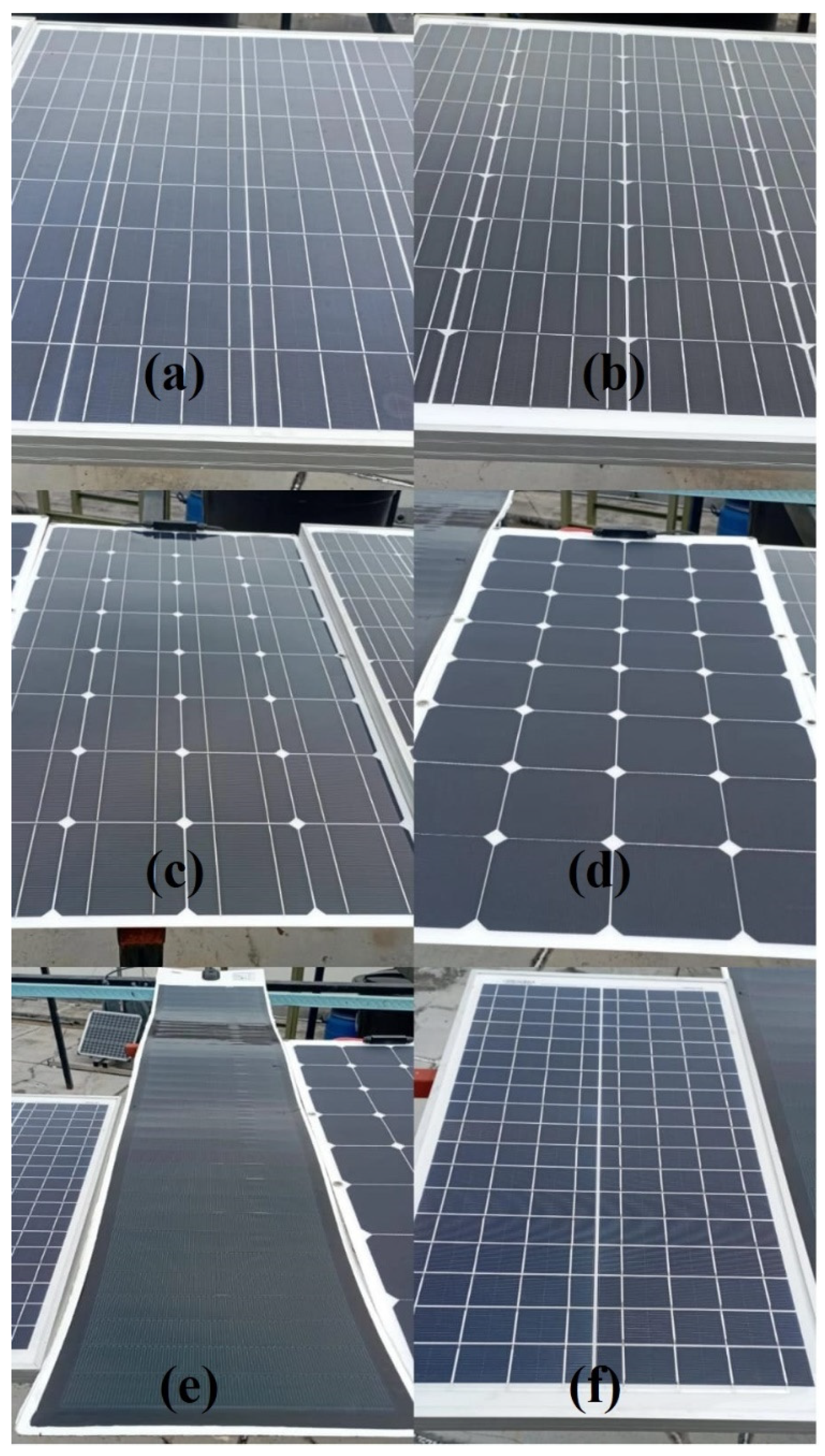
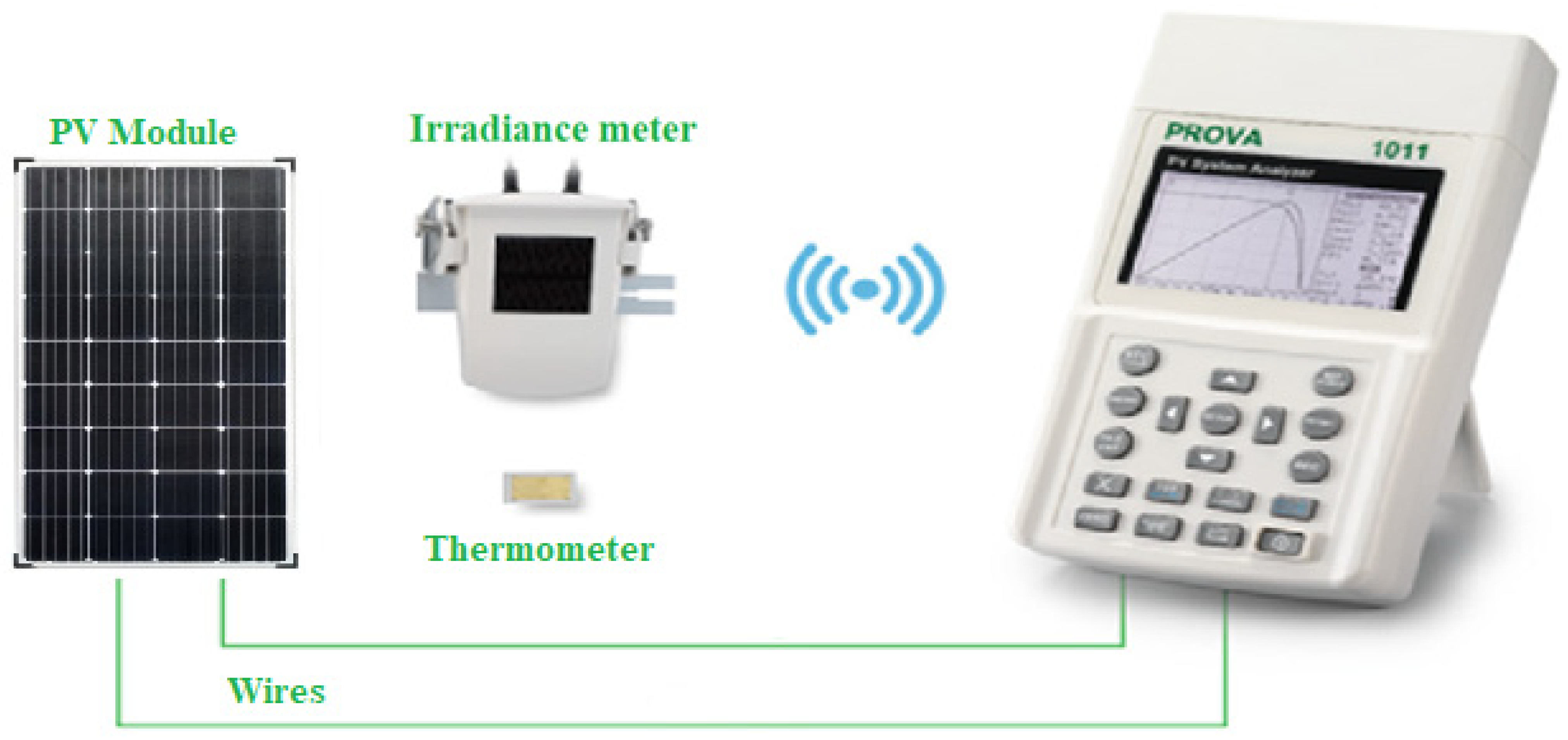
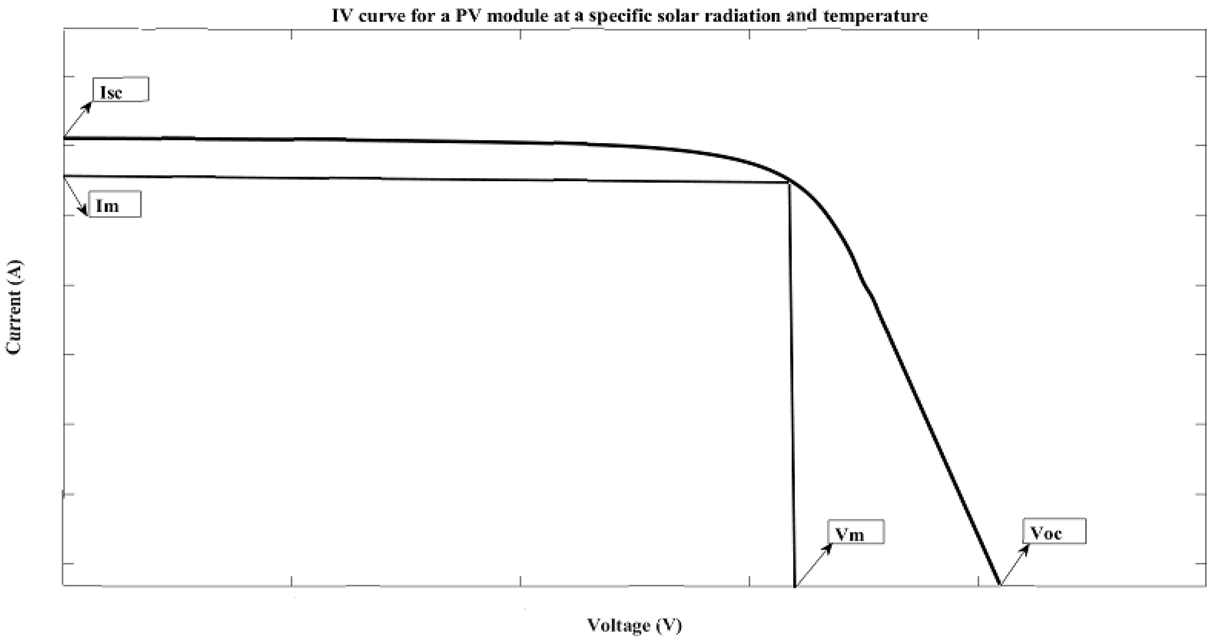
2. Experimental Setup and Major Parameters of the PV Module

During this research, six different types of PV panels were used to collect data using a Prova 1011 solar system analyzer, namely, a polycrystalline panel (100 W), a monocrystalline panel (100 W), a flexible mono-panel (100 W), a thin-film amorphous panel (100 W), a CIGS solar panel (90 W), and a flexible back-contact mono-panel (30 W). Figure 1 shows the six PV modules’ visual images while collecting the dataset.
The Prova 1011 solar system analyzer was used to measure the PV module performance (IV curve), FF, Pm (Vm and Im), and efficiency under different test conditions. The instrument connects with a wireless irradiance meter and thermometer to collect the irradiance and cell temperature under the test conditions for the PV modules, as shown in Figure 2. Moreover, the device can calculate the efficiencies and the maximum power under test conditions by saving the specification of the PV module (area, Voc, and Isc) by connecting the device with a special software program for the device. After that, a considerable number of IV curves at different irradiance and temperature for the six PV modules are extracted from the device, and the software is used during the MATLAB program’s training process.
An IV curve can represent the relationship between the current (the vertical axis of the curve) and voltage (the horizontal axis of the curve) at a specific irradiance and temperature, as shown in Figure 3. Analyzing the figure shows several essential points in the IV curve. As shown in Equation (1), the Isc represents the highest current produced when the voltage is zero.
I   ( at   V = 0 ) = I sc
Secondly, as shown in Equation (2), Voc represents the highest voltage produced when the current is zero.
V   ( at   I = 0 ) = V oc
Other essential points and parameters for this research include the maximum power point (MPPT). This represents the point in the IV curve where the rectangle area below the IV curve is the maximum. At the same time, the efficiency is the ratio between Pm and the input power (Pin). Pin is the product of the solar cell irradiation of the incident light. Lastly, the FF is the ratio between Pm and the product of Isc and Voc. These important parameters can be given by Equations (3)–(5) [40,41]:
  P m =   I m   .   V m
η = P m   / P in
FF = P m     I sc . V oc

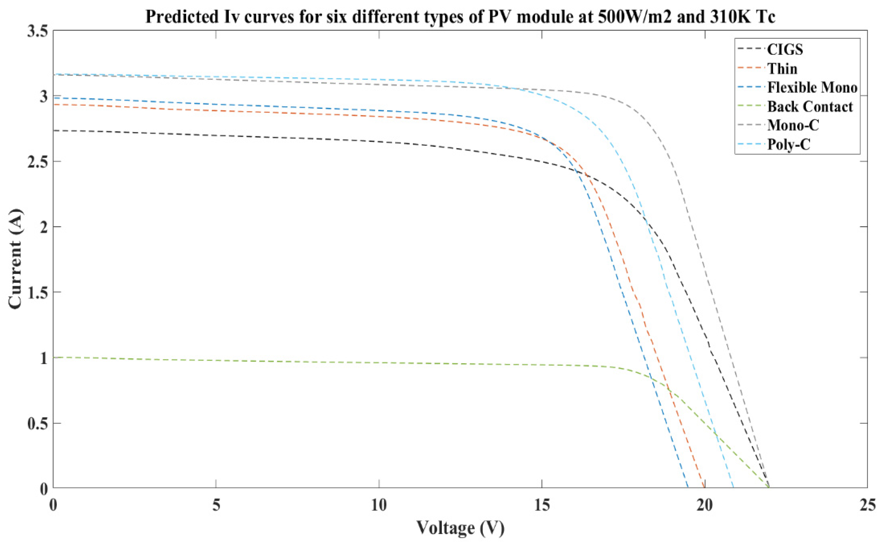
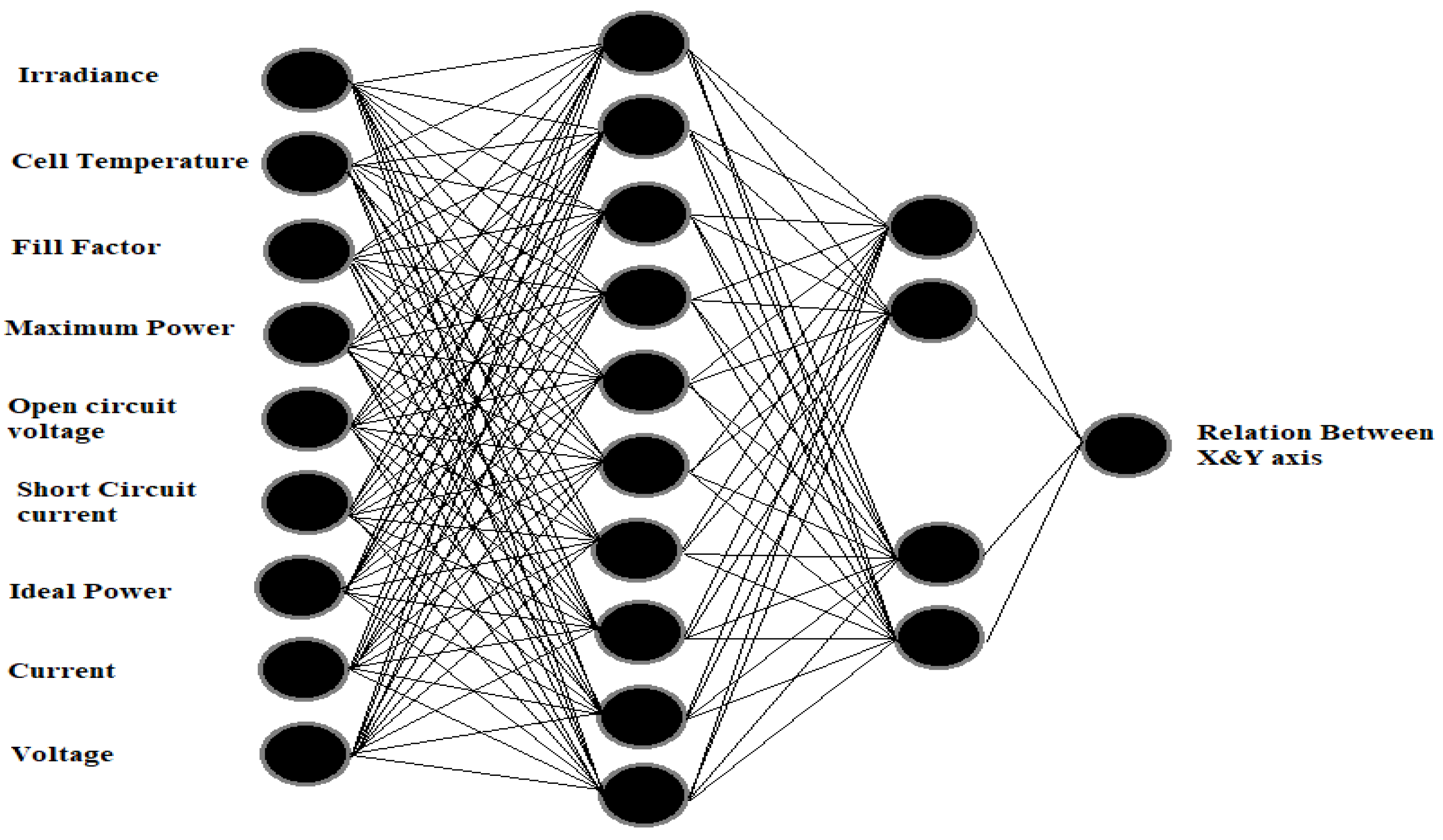
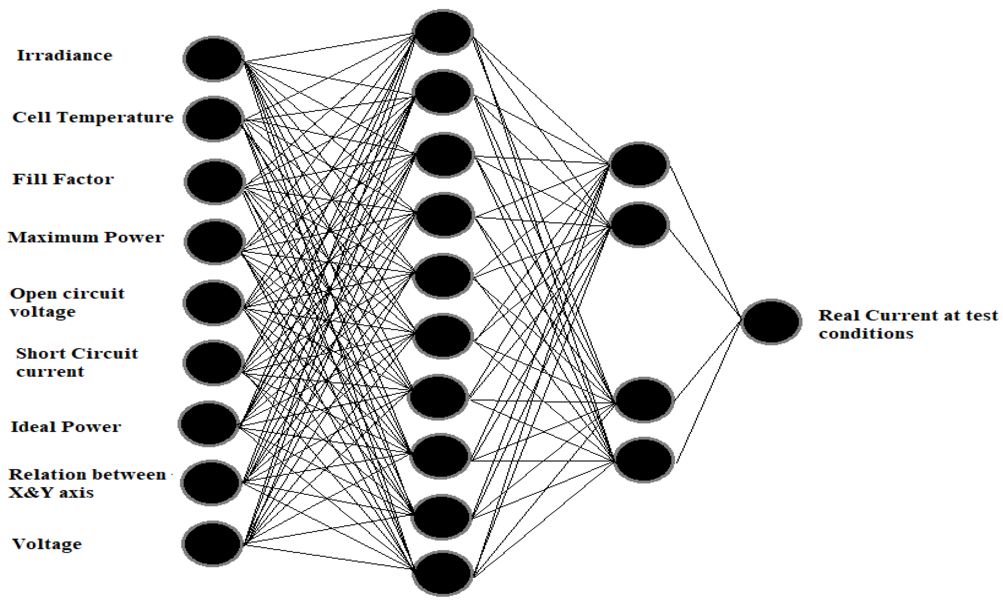
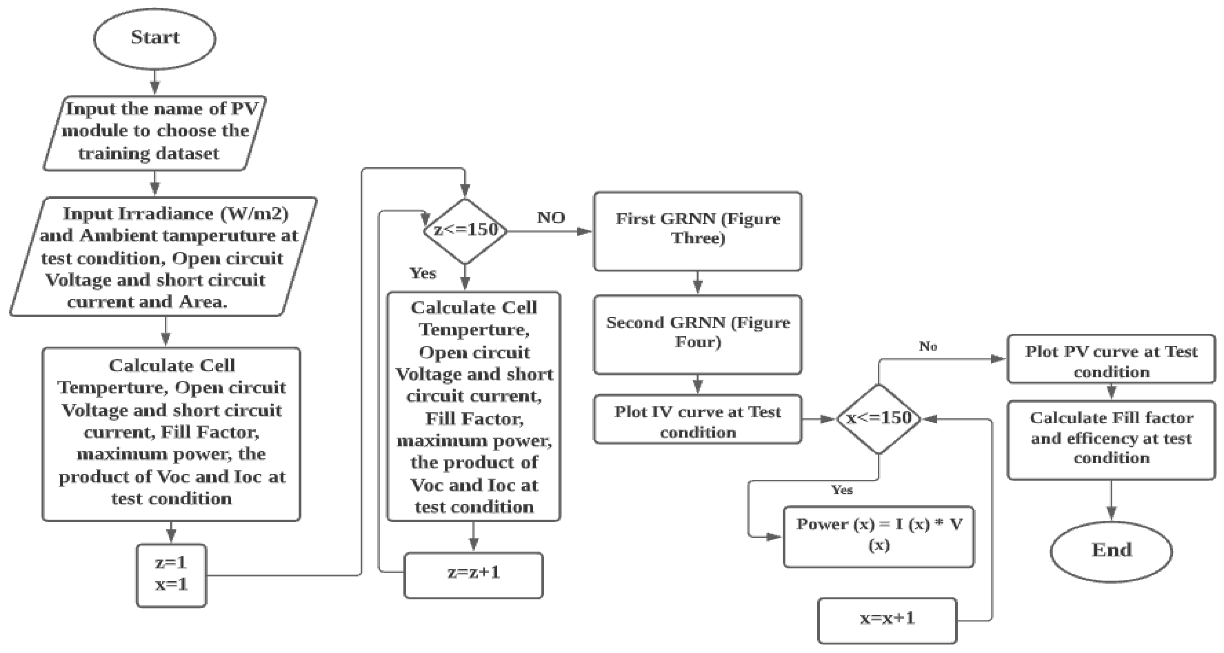
3. Proposed ANNs Model for Predicting the Performance of the Six PV Modules

Artificial neural networks (ANNs) are non-algorithm information-processing systems that use previously collected data to train the networks to predict specific variables such as current, efficiency, output power, and solar radiation [42]. Every network, in general, has three types of layers, input, hidden, and output layers [42,43].
There are two generalized regression neural networks (GRNNs) that predict the IV curve. The output for the first GRNN is used as an input variable in the second GRNN; the second network predicts the current of one of the six PV modules at specific conditions. The architecture, and the number of neurons in the input, hidden, and output layers, are the same for both networks. Moreover, each training dataset has one neuron for every input with different values and weights. The input neurons in this proposed model feed their values to the neurons in the hidden layer. After multiplying the values with a target, the final value is transferred to the neurons in the pattern layer. In this layer, the final values are added by weights from each hidden neuron, and the result is used as the predicted value [30]. In this research, the mechanism recorded IV curves for the proposed ANNs method using a Prova 1011 Solar System Analyzer. The device extracted a considerable number of IV curves at different irradiances and temperatures for the six PV modules. Most of these IV curve data were sent for the training process for the proposed ANNs method. Simultaneously, some of them were used during the testing process of the method.
In the proposed model, the first GRNN is trained by IV curve data for six different types of PV modules at different irradiances and cell temperatures, with FF, Pmax, Isc, Voc, voltage, current, and the product of Isc and Voc. These factors are used as input for the training process in the first network. The output for the first GRNN represents the relation between current and voltage. The training method’s inputs contain specialized information for one of the six PV modules covered by the device. Figure 4 shows the first proposed GRNN used in the model.
The testing process for the first GRNN starts by obtaining the current and voltage for the PV module by stepping their highest value down. These parameters are used as an input for the testing process with irradiance, cell temperature (Tc), FF, Pmax, a product of Isc and Voc, Isc, and Voc to predict a parameter representing the relation between the x-axis and the y-axis. Meanwhile, the second GRNN predicts the current for one of the six types of modules at specific irradiance and temperature. The inputs for the training process are irradiance, Tc, voltage, a product of Isc and Voc, FF, Pmax, Isc, Voc, and the output parameter from the first GRNN. The inputs for the testing process for the network are the same as the training process. Figure 5 shows the second GRNN proposed in this model. The proposed model starts by entering the name of the PV module with the specifications of the module. A “for loop” is used to upload the training dataset for the same PV module, depending on the type of PV module chosen. After this, the test conditions for the PV module (irradiance and Tc) should be specified. Then, the datasheet for the PV module is used to calculate Isc and Voc under test conditions using Equations (6) and (7) as below [42]:
V oc T =   V oc stc ( ( T c T a ) ) × 0.123 )
  I sc T = I sc stc × ( Irradiance   at   the   test   condition Irradiance   at   STC )
Before the testing process, another “for loop” is used to create the testing data input. The inputs are the same as those used during the training process. The last two inputs are calculated by stepping down Isc and Voc. As shown in Figure 5, the first GRNN is utilized as an input for the second GRNN, which predicts the relationship between the x-axis and y-axis in the IV curve. The second GRNN, as shown in Figure 5, predicts the current and extracts the IV and PV curves. Finally, after repeating the same process with the same test conditions for the six different PV modules, the output data from each test condition are used to calculate the efficiency and FF to compare how each PV module performs under the same test conditions in Malaysia. Figure 6 shows the flowchart of the proposed model process.
For this research, the accuracy of the predicted performance was evaluated by using three types of errors: first, the mean absolute deviation (MAD). This error is an indication to measure the dispersal of a specific set of data and is calculated using Equation (8):
  MAD = 1 n i = 1 r | x p m ( X ) |
where r is the number of the value, xi is the predicted value from the proposed model, and m(X) is the dataset’s average. Secondly, the mean absolute percentage error (MAPE) was used, which can be given by Equation (9):
  MAPE = Experimental   Value Predicted   Value Experimental   Value × 100 %
This is usually used for calculating the accuracy of the new value (predicted value). Lastly, the root mean square error (RMSE) was used, which indicates the short-term performance and is calculated by using Equation (10):
RMSE = 1 n i = 1 r ( x p x e ) 2                        
where xe is the experimental value. MAPE was used to calculate the percentage of error of the predicting result to the experimental result. However, the results of the MAPE cannot always indicate the real error if the value of the prediction is too small. Therefore, types of errors such as RMSE and MAD are useful for this research.

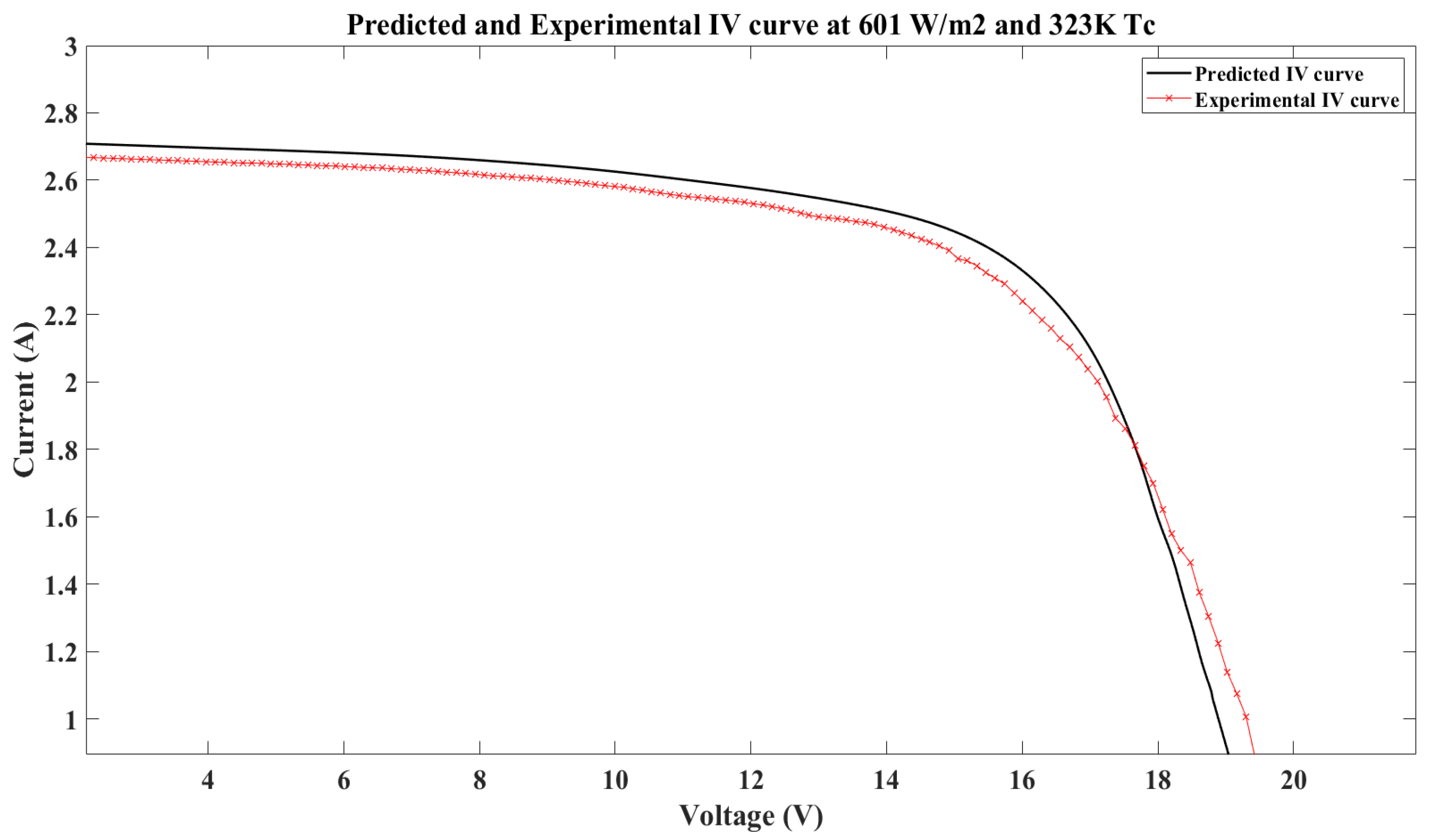
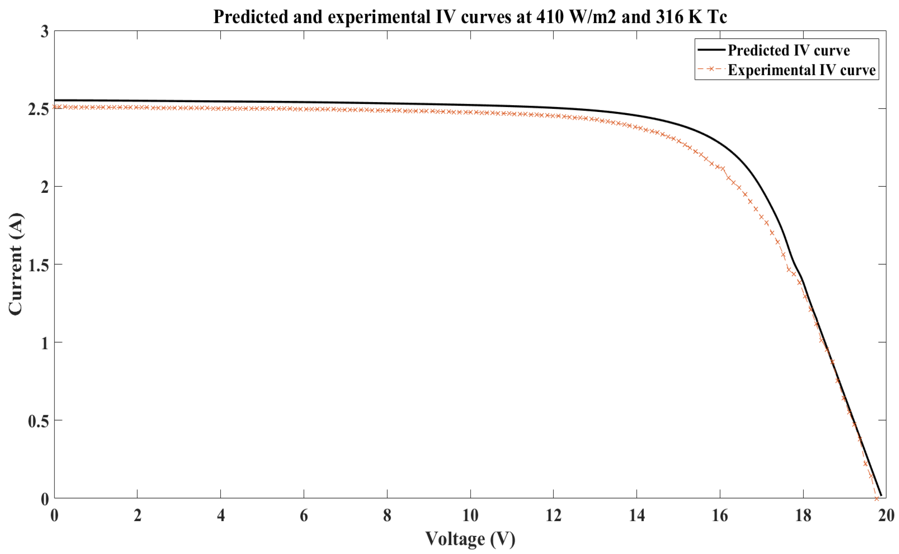
4. Result and Discussion

In this research, six different types of PV modules were used to collect datasets for the training and testing process of the ANN by a Prova 1011 solar system analyzer. The technical characteristics of the PV modules at STC are described in Table 2.
There are 37,144 records for 247 IV curves that have been collected from the six PV modules, 40 IV curves from the flexible back-contact mono-module, 50 curves from the CIGS module, 42 curves from the thin-film module, 40 IV curves from the flexible mono-module, 35 curves from monocrystalline module, and 40 curves from polycrystalline module. Each record has a value for voltage, current, Voc, Isc, FF, a product of Isc and Voc, irradiance, Tc, and Pmax. A total of 7.69% of the dataset was used for the testing process, while the remaining data were used during the training process.
For the prediction process, the proposed model predicted the IV curve for the six different PV modules by entering the name of the PV module and the specific desired test conditions, as explained in Figure 6. To test the accuracy of the proposed model under different test conditions, each predicted IV curve has a different solar radiation level and ambient temperature for each PV module. Figure 7, Figure 8, Figure 9, Figure 10, Figure 11 and Figure 12 show the predicted IV curves with the experimental IV curves for the six modules that were extracted. For each predicted IV curve, the proposed model starts the process of training and predicting from the start, as shown in the flowchart in Figure 6.
After this, to compare the prediction performance of the six PV modules under test conditions and how each PV module will perform under the same test conditions, the proposed model predicted the IV and PV curves for the six different types of PV modules under the same test conditions, as explained in Figure 6. Figure 13, Figure 14, Figure 15 and Figure 16 compare and show the predicted IV and PV curves for the six modules under the same test conditions. All the graphs were created using the MATLAB program.
From Figure 13, Figure 14, Figure 15 and Figure 16, FF efficiency for the six modules under the same test conditions were calculated, as shown in Table 3. The highest FF is the monocrystalline module, with an average of 0.737, while the lowest FF is the CIGS module, with an average of 0.66. For efficiency, the highest is the monocrystalline module, with an average of 10.32%, while the lowest is the thin-film module, with an average of 7.65%. Both thin-film and flexible mono-modules have similar performances.
From Table 4, by using Equations (8)–(10), the overall prediction accuracy of the proposed model was shown to have an average root mean square error (RMSE) and mean absolute deviation (MAD) of 0.0638 A and 0.237 A, respectively, while the average accuracy of the mean absolute percentage error (MAPE) is 0.874%. The accuracy of the proposed model proved its efficiency compared to the previous models presented in Table 1.
From the results in Table 3 and Table 4, the proposed model predicted and compared the performance of the six different PV modules under test conditions with an accuracy of 99.126%, which is higher than of the all offline and online methods represented in Table 1. The model needs less than 30 s after entering the specific test conditions to predict the performance of the PV module by using and asking for simple parameters such as irradiance, Voc, and Isc of the PV module.

5. Conclusions

This research proposed a model for comparing the prediction performance (IV curves, efficiency, and FF) of six different PV modules using an ANN. The ANN that is used for this model is a generalized regression neural network (GRNN). The model inputs for the ANN are irradiance, Tc, a product of Isc and Voc, FF, and the technical characteristics of the six PV modules. In this research, 37,144 records for 247 IV curves were collected from the six PV modules under different test conditions. The MATLAB program was used to train and test the data that were extracted from the device. Under the test conditions in Malaysia (solar radiation and ambient temperature), the monocrystalline module had the highest FF and efficiency, while the CIGS module had the lowest FF. As for efficiency, the lowest was the thin-film module. The overall prediction accuracy for the proposed model has an RMSE and MAD of 0.0638 A and 0.237 A, respectively. At the same time, the accuracy of the MAPE is 0.874%. In future, a different device with a higher accuracy for collecting training data sets and more variation in the training data and test conditions could improve the accuracy of the proposed model. These results proved the accuracy of the model for predicting the performance of the six PV modules.

Author Contributions

Data curation, M.J.; Supervision, K.S., A.F. and A.I.; Conceptualization, K.S., A.I. and M.J.; Formal analysis, M.J.; Software, M.J.; Investigation, A.S.A.H., K.S., A.I. and M.J.; Methodology, M.J.; Validation, M.J.; Writing—original draft, M.J.; Writing—review editing, A.S.A.H., A.I., A.F. and K.S. All authors have read and agreed to the published version of the manuscript.

Funding

This research was funded by the Program Translational MRUN Rakan-RU-2019-001/4 (Universiti Kebangsaan Malaysia) and SPBK-UMS phase 1/2022 (SBK0518-2022-Universiti Malaysia Sabah) research grants. The APC was funded by Universiti Malaysia Sabah.

Data Availability Statement

Not applicable.

Acknowledgments

The authors would like to acknowledge the Solar Energy Research Institute, Universiti Kebangsaan Malaysia (UKM) and Faculty of Science and Natural Resources, Universiti Malaysia Sabah (UMS) for the lab facilities. This research was supported by FRGS/1/2019/TK07/UKM/02/4 (UKM) and SPBK-UMS phase 1/2022 (SBK0518-2022) (UMS) research grants.

Conflicts of Interest

The authors declare no conflict of interest.

Abbreviations

PVPhotovoltaic
IVCurrent–voltage
BIPVBuilding-integrated photovoltaic
IscShort-circuit current
VocOpen-circuit voltage
TcCell temperature
FFFill factor
PRPerformance ratio
MPPTMaximum power point
PmMaximum power
ImMaximum current
VmMaximum voltage
PinInput power
ηEfficiency
ANNsArtificial neural networks
AIArtificial intelligence
GAGenetic algorithm
RNNRecurrent neural network
GRNNGeneralized regression neural network
Voc_TOpen-circuit voltage under test conditions
Voc_STCOpen-circuit voltage under standard test conditions
TaAmbient temperature
Isc_TShort-circuit current under test conditions
Isc_STCShort-circuit current under standard test conditions
MAPEMean absolute percentage error
rNumber of the value
xiPredicted value
m(X)Dataset’s average
RMSERoot mean square error
MADMean absolute deviation
xeExperimental value

References

  1. Sukarno, K.; Hamid, A.S.A.; Jackson, C.H.W.; Pien, C.F.; Dayou, J. Comparison of power output between fixed and perpendicular solar photovoltaic PV panel in tropical climate region. Adv. Sci. Lett. 2017, 23, 1259–1263. [Google Scholar] [CrossRef]
  2. Parida, B.; Iniyan, S.; Goic, R. A review of solar photovoltaic technologies. Renew. Sustain. Energy Rev. 2011, 15, 1625–1636. [Google Scholar] [CrossRef]
  3. Baljit, S.S.S.; Chan, H.-Y.; Sopian, K. Review of building integrated applications of photovoltaic and solar thermal systems. J. Clean. Prod. 2016, 137, 677–689. [Google Scholar] [CrossRef]
  4. Fudholi, A.; Sopian, K.; Yazdi, M.H.; Ruslan, M.H.; Ibrahim, A.; Kazem, H.A. Performance analysis of photovoltaic thermal (PVT) water collectors. Energy Convers. Manag. 2014, 78, 641–651. [Google Scholar] [CrossRef]
  5. Abdul Hamid, S.; Yusof Othman, M.; Sopian, K.; Zaidi, S.H. An overview of photovoltaic thermal combination (PV/T combi) technology. Renew. Sustain. Energy Rev. 2014, 38, 212–222. [Google Scholar] [CrossRef]
  6. Abd Hamid, A.S.; Makmud, M.Z.H.; Abd Rahman, A.B.; Jamain, Z.; Ibrahim, A. Investigation of Potential of Solar Photovoltaic System as an Alternative Electric Supply on the Tropical Island of Mantanani Sabah Malaysia. Sustainability 2021, 13, 12432. [Google Scholar] [CrossRef]
  7. Sukarno, K.; Hamid, A.S.A.; Razali, H.; Dayou, J. Evaluation on cooling effect on solar PV power output using Laminar H2O surface method. Int. J. Renew. Energy Res. 2017, 7, 1213–1218. [Google Scholar]
  8. Abd Hamid, A.S.; Ibrahim, A.; Mat, S.; Sukarno, K.; Dayou, J. Evaluation on Low Temperature and Tracking Effect of Solar Photovoltaic Power Output Under Tropical Climate Condition in Kota Kinabalu, Malaysia. In Proceedings of the 2nd Malaysia University-Industry Green Building Collaboration Symposium (MU-IGBC 2018), Bangi, Malaysia, 8 May 2018; pp. 227–231. [Google Scholar]
  9. Darwish, Z.A.; Kazem, H.A.; Sopian, K.; Al-Goul, M.A.; Alawadhi, H. Effect of dust pollutant type on photovoltaic performance. Renew. Sustain. Energy Rev. 2015, 41, 735–744. [Google Scholar] [CrossRef]
  10. Darwish, Z.A.; Sopian, K.; Fudholi, A. Reduced output of photovoltaic modules due to different types of dust particles. J. Clean. Prod. 2021, 280, 124317. [Google Scholar] [CrossRef]
  11. Mirzaei, M.; Mohiabadi, M.Z. A comparative analysis of long-term field test of monocrystalline and polycrystalline PV power generation in semi-arid climate conditions. Energy Sustain. Dev. 2017, 38, 93–101. [Google Scholar] [CrossRef]
  12. Silvestre, S.; Tahri, A.; Tahri, F.; Benlebna, S.; Chouder, A. Evaluation of the performance and degradation of crystalline silicon-based photovoltaic modules in the Saharan environment. Energy 2018, 152, 57–63. [Google Scholar] [CrossRef]
  13. Ram, J.P.; Manghani, H.; Pillai, D.S.; Babu, T.S.; Miyatake, M.; Rajasekar, N. Analysis on solar PV emulators: A review. Renew. Sustain. Energy Rev. 2018, 81, 149–160. [Google Scholar] [CrossRef]
  14. Malik, A.Q.; Damit, S.J.B.H. Outdoor testing of single crystal silicon solar cells. Renew. Energy 2003, 28, 1433–1445. [Google Scholar] [CrossRef]
  15. Van Dyk, E.E.; Gxasheka, A.R.; Meyer, E.L. Monitoring current–voltage characteristics and energy output of silicon photovoltaic modules. Renew. Energy 2005, 30, 399–411. [Google Scholar] [CrossRef]
  16. Muñoz, J.; Lorenzo, E. Capacitive load based on IGBTs for on-site characterization of PV arrays. Sol. Energy 2006, 80, 1489–1497. [Google Scholar] [CrossRef] [Green Version]
  17. Forero, N.; Hernández, J.; Gordillo, G. Development of a monitoring system for a PV solar plant. Energy Convers. Manag. 2006, 47, 2329–2336. [Google Scholar] [CrossRef]
  18. Kuai, Y.; Yuvarajan, S. An electronic load for testing photovoltaic panels. J. Power Sources 2006, 154, 308–313. [Google Scholar] [CrossRef]
  19. Duran, E.; Galan, J.; Sidrach-de-Cardona, M.; Andujar, J.M. A New Application of the Buck-Boost-Derived Converters to Obtain the I-V Curve of Photovoltaic Modules. In Proceedings of the 2007 IEEE Power Electronics Specialists Conference, Orlando, FL, USA, 17–21 June 2007; pp. 413–417. [Google Scholar]
  20. Khatib, T.; Elmenreich, W.; Mohamed, A. Simplified I–V Characteristic Tester for Photovoltaic Modules Using a DC-DC Boost Converter. Sustainability 2017, 9, 657. [Google Scholar] [CrossRef] [Green Version]
  21. Bai, J.; Liu, S.; Hao, Y.; Zhang, Z.; Jiang, M.; Zhang, Y. Development of a new compound method to extract the five parameters of PV modules. Energy Convers. Manag. 2014, 79, 294–303. [Google Scholar] [CrossRef]
  22. Ma, T.; Yang, H.; Lu, L. Development of a model to simulate the performance characteristics of crystalline silicon photovoltaic modules/strings/arrays. Sol. Energy 2014, 100, 31–41. [Google Scholar] [CrossRef]
  23. Navabi, R.N.; Abedi, S.; Hosseinian, S.H.; Pal, R. On the fast convergence modeling and accurate calculation of PV output energy for operation and planning studies. Energy Convers. Manag. 2015, 89, 497–506. [Google Scholar] [CrossRef]
  24. Ismail, M.S.; Moghavvemi, M.; Mahlia, T.M.I. Characterization of PV panel and global optimization of its model parameters using genetic algorithm. Energy Convers. Manag. 2013, 73, 10–25. [Google Scholar] [CrossRef]
  25. Dizqah, A.M.; Maheri, A.; Busawon, K. An accurate method for the PV model identification based on a genetic algorithm and the interior-point method. Renew. Energy 2014, 72, 212–222. [Google Scholar] [CrossRef] [Green Version]
  26. Jiang, L.L.; Maskell, D.L.; Patra, J.C. Parameter estimation of solar cells and modules using an improved adaptive differential evolution algorithm. Appl. Energy 2013, 112, 185–193. [Google Scholar] [CrossRef]
  27. Muhsen, D.H.; Ghazali, A.B.; Khatib, T.; Abed, I.A. A comparative study of evolutionary algorithms and adapting control parameters for estimating the parameters of a single-diode photovoltaic module’s model. Renew. Energy 2016, 96, 377–389. [Google Scholar] [CrossRef]
  28. Sukarno, K.; Abd Hamid, A.S.; Dayou, J.; Makmud, M.Z.H.; Sarjadi, M.S. Measurement of global solar radiation in Kota Kinabalu Malaysia. ARPN J. Eng. Appl. Sci. 2015, 10, 6467–6471. [Google Scholar]
  29. Hamid, A.S.A.; Ibrahim, A.; Assadeg, J.; Ahmad, E.Z.; Sopian, K. Techno-economic Analysis of a Hybrid Solar Dryer with a Vacuum Tube Collector for Hibiscus Cannabinus L Fiber. Int. J. Renew. Energy Res. 2020, 10, 1609–1613. [Google Scholar]
  30. Khatib, T.; Mohamed, A.; Sopian, K.; Mahmoud, M. Assessment of Artificial Neural Networks for Hourly Solar Radiation Prediction. Int. J. Photoenergy 2012, 2012, 946890. [Google Scholar] [CrossRef]
  31. El-kenawy, E.M.T. Solar Radiation Machine Learning Production Depend on Training Neural Networks with Ant Colony Optimization Algorithms. Int. J. Adv. Res. Comput. Commun. Eng. 2018, 7, 1–4. [Google Scholar]
  32. Sivaneasan, B.; Yu, C.Y.; Goh, K.P. Solar Forecasting using ANN with Fuzzy Logic Pre-processing. Energy Procedia 2017, 143, 727–732. [Google Scholar] [CrossRef]
  33. Khatib, T.; Ghareeb, A.; Tamimi, M.; Jaber, M.; Jaradat, S. A new offline method for extracting I-V characteristic curve for photovoltaic modules using artificial neural networks. Sol. Energy 2018, 173, 462–469. [Google Scholar] [CrossRef]
  34. Zhang, C.; Zhang, Y.; Su, J.; Gu, T.; Yang, M. Performance prediction of PV modules based on artificial neural network and explicit analytical model Performance prediction of PV modules based on artificial neural network and explicit analytical model. J. Renew. Sustain. Energy 2020, 12, 013501. [Google Scholar] [CrossRef]
  35. Mittal, M.; Bora, B.; Saxena, S.; Mli, A. Performance prediction of PV module using electrical equivalent model and artificial neural network. Sol. Energy 2018, 176, 104–117. [Google Scholar] [CrossRef]
  36. Ibrahim, I.A.; Hossain, M.J.; Member, S.; Duck, B.C. An Optimized Offline Random Forests-Based Model for Ultra-short-term Prediction of PV Characteristics. IEEE Trans. Ind. Inform. 2019, 16, 202–214. [Google Scholar] [CrossRef]
  37. Theocharides, S.; Makrides, G.; George, E.; Kyprianou, A. System Power Output Prediction. In Proceedings of the 2018 IEEE International Energy Conference (ENERGYCON), Limassol, Cyprus, 3–7 June 2018; pp. 1–6. [Google Scholar]
  38. Jung, Y.; Jung, J.; Kim, B.; Han, S. Long short-term memory recurrent neural network for modeling temporal patterns in long-term power forecasting for solar PV facilities: Case study of South Korea. J. Clean. Prod. 2020, 250, 119476. [Google Scholar] [CrossRef]
  39. Khandakar, A.; Chowdhury, M.E.H.; Kazi, M.-K.; Benhmed, K.; Touati, F.; Al-hitmi, M.; Gonzales, A.J.S.P. Machine Learning Based Photovoltaics (PV) Power Prediction Using Different Environmental Parameters of Qatar. Energies 2019, 12, 2782. [Google Scholar] [CrossRef] [Green Version]
  40. Castaner, L.; Silvestre, S. Modelling Photovoltaic Systems Using PSpice; John Wiley and Sons: Hoboken, NJ, USA, 2003; ISBN 9780470855539. [Google Scholar]
  41. Mosaad, M.I.; abed el-Raouf, M.O.; Al-Ahmar, M.A.; Banakher, F.A. Maximum Power Point Tracking of PV system Based Cuckoo Search Algorithm; review and comparison. Energy Procedia 2019, 162, 117–126. [Google Scholar] [CrossRef]
  42. Dagli, C.H.; Buczak, A.L.; Ghosh, J.; Embrechts, M.J.; Ersoy, O.; Kercel, S. Intelligent Engineering Systems through Artificial Neural Networks: Volume 10, Fuzzy Logic and Evolutionary Programming; American Society of Mechanical Engineers ASME: New York, NY, USA, 2000; ISBN 0791801616. [Google Scholar]
  43. Butler, C.; Caudill, M. Understanding Neural Networks—IBM Version, Volume 1: Basic Networks; The MIT Press: Cambridge, MA, USA, 1993; ISBN 9780262530996. [Google Scholar]
Figure 1. (a) Polycrystalline panel, (b) monocrystalline panel, (c) flexible mono-panel, (d) thin-film amorphous panel, (e) CIGS solar panel, and (f) flexible back-contact mono-panel.
Applsci 12 03349 g001
Figure 2. Set-up for extracting IV curves by Prova 1011 solar system analyzer.
Applsci 12 03349 g002
Figure 3. IV curve for a PV module.
Applsci 12 03349 g003
Figure 4. The first proposed GRNN flowchart to predict the relation between the X and Y axes.
Applsci 12 03349 g004
Figure 5. The second proposed GRNN flowchart to predict the real current.
Applsci 12 03349 g005
Figure 6. Flowchart of the proposed model process.
Applsci 12 03349 g006
Figure 7. Predicted and experimental IV curves for CIGS module at 601 W/m2 and 323 K Tc.
Applsci 12 03349 g007
Figure 8. Predicted and experimental IV curves for thin module at 586 W/m2 and 312 K Tc.
Applsci 12 03349 g008
Figure 9. Predicted and experimental IV curves for flexible mono-module at 864 W/m2 and 314 K Tc.
Applsci 12 03349 g009
Figure 10. Predicted and experimental IV curves for polycrystalline module at 410 W/m2 and 316 K Tc.
Applsci 12 03349 g010
Figure 11. Predicted and experimental IV curves for monocrystalline module at 640 W/m2 and 324 K Tc.
Applsci 12 03349 g011
Figure 12. Predicted and experimental IV curves for flexible back-contact mono-module at 865 W/m2 and 312 K Tc.
Applsci 12 03349 g012
Figure 13. Predicted IV curves for the six PV modules at 650 W/m2 and 315 K Tc.
Applsci 12 03349 g013
Figure 14. Predicted IV curves for the six PV modules at 500 W/m2 and 310 K Tc.
Applsci 12 03349 g014
Figure 15. Predicted PV curves for the six PV modules at 650 W/m2 and 315 K Tc.
Applsci 12 03349 g015
Figure 16. Predicted PV curves for the six PV modules at 500 W/m2 and 310 K Tc.
Applsci 12 03349 g016
Table 2. The technical characteristics at STC.
Types of PV ModulePmVocIscVmIm
CIGS 90 W26.4 V5.1 A21 V4.5 A
Thin film 100 W20 V5.6 A18 V5.1 A
Flexible mono 100 W19.2 V5.68 A16 V5.15 A
Polycrystalline 100 W21.42 V5.76 A18.59 V5.38 A
Monocrystalline 100 W21.97 V6.07 A17.46 V5.73 A
Flexible back-contact Mono 30 W21.97 V1.75 A18.31 V1.64 A
Table 3. FF and efficiency for the six PV modules under the same test conditions.
Type of PV ModuleCell
Temperature (K)
Irradiance
(W/m2)
FFEfficiency (%)
CIGS3156500.6678459.6274
3105000.654548.7328
Thin film3156500.6764998.083
3105000.6856787.223
Flexible mono3156500.6776298.0899
3105000.6988357.323
Polycrystalline3156500.69692110.9832
3105000.7025588.4353
Monocrystalline3156500.7312411.2789
3105000.7428759.3722
Flexible back-contact mono3156500.717448.828
3105000.7254627.2522
Table 4. Values of MAD, MAPE, and RMSE under different test conditions for the six PV modules.
Type of PV ModuleIrradiance (W/m2)Tc (K)MADMAPE (%)RMSE
Flexible back-contact mono5473120.1120.5320.026
CIGS7163210.2630.5170.080
Polycrystalline5503100.3931.1730.092
Flexible back-contact mono6953080.1540.3470.034
Thin film4013100.1980.8720.052
Flexible mono3953140.2320.9850.064
Flexible back-contact mono8653150.1961.0690.035
Monocrystalline7503270.341.1860.098
CIGS8403150.2370.9530.075
Polycrystalline4733110.2481.0650.082
Thin film5703130.1740.7750.041
Monocrystalline3803080.2911.0240.087
Publisher’s Note: MDPI stays neutral with regard to jurisdictional claims in published maps and institutional affiliations.

