Genetic Algorithm versus Discrete Particle Swarm Optimization Algorithm for Energy-Efficient Moving Object Coverage Using Mobile Sensors

Abstract

This paper addresses the challenge of moving objects in a mobile wireless sensor network, considering the deployment of a limited number of mobile wireless sensor nodes within a predetermined area to provide coverage for moving objects traveling on a predetermined trajectory. Because of the insufficient number and limited sensing range of mobile wireless sensors, the entire object’s trajectory cannot be covered by all deployed sensors. To address this problem and provide complete coverage, sensors must move from one point of the trajectory to another. The frequent movement quickly depletes the sensors’ batteries. Therefore, solving the moving object coverage problem requires an optimized movement repertoire where (1) the total moving distance is minimized and (2) the remaining energy is also as balanced as possible for mobile sensing. Herein, we used a genetic algorithm (GA) and a discrete particle swarm optimization algorithm (DPSO) to manage the complexity of the problem, compute feasible and quasi-optimal trajectories for mobile sensors, and determine the demand for movement among nodes. Simulations revealed that the GA produced trajectories significantly superior to those produced by the DPSO in terms of total traveled distance and balance of residual energy.

1. Introduction

A wireless sensor network (WSN) is composed of hundreds or thousands of tiny sensors with sensing and communication capabilities [1]. These sensors can monitor and detect aspects of their surrounding environment, and such data can be transmitted and communicated to other sensors or base stations, enabling coordination for the completion of specific tasks. WSNs are used extensively in numerous fields, including environmental monitoring, military operations, medicine, smart homes, animal conservation, and poaching prevention. In object tracking, a key application of WSNs—and the focus of this study—a group of sensors is deployed in a predetermined area to monitor the position, speed, and trajectory of objects (among other related characteristics). This collected information is then delivered to related base stations within a specified period of time for further application. Unlike global positioning systems, WSNs can leverage various sensing technologies (e.g., ultrasonic, infrared, electromagnetic, and laser sensors) to locate objects quickly and accurately [2]. Furthermore, sensors can identify an object and monitor its status.

Because WSNs are compact, using them to achieve sufficient computing power and communication range is difficult. Energy consumption is the most critical constraint. WSNs can fail to connect if many sensors are depleted of energy. To achieve the requisite coverage in such circumstances, mobile sensors may need to be moved to suitable positions.

Mobile sensors have become smaller and cheaper with advances in technology. For example, in [3], the researchers introduced a mobile sensor called Robomote. Occupying less than 0.000047 m³ of space and costing less than $150, it was developed to explore problems in large-scale sensor networks. Although small and inexpensive, mobile sensors consume energy, and a mobile sensor consumes the most energy when it moves. The amount of energy consumed by a mobile sensor is usually related to the distance the sensor travels. Therefore, reducing the moving distance is a critical challenge for reducing energy consumption.

In this study, we addressed the moving object coverage problem in a WSN by using a limited number of mobile sensors. This problem occurs when the full tracking of an object traveling on a predetermined trajectory in a specified area is required, but because of the insufficient number and limited sensing range of mobile wireless sensors, the object trajectory cannot be entirely covered by the deployed sensors. Thus, the mobile sensors must move from one position on the trajectory to another to achieve complete coverage. To conserve energy, a mobile sensor movement repertoire that minimizes the total traveled distance must be determined. Furthermore, to prolong the network lifetime, the remaining power of each mobile sensor must also be as balanced as possible. The complexity of the problem has grown due to the multiple objectives that must be achieved. In attempting to solve such a complex problem, traditional heuristic algorithms often can only obtain an approximate solution close to the optimal solution, and should only be used to solve smaller problems. In solving larger and more complex problems, the solution precision of traditional heuristic algorithms is poor and meta-heuristic algorithms should be used instead because of their strong global search performance. In a preliminary work [4], we addressed the key design aspect of using a genetic algorithm (GA) to identify optimal or near-optimal solutions to the moving object coverage problem with a small problem size. In this paper, we extend our previous work by mathematically formulating the moving object coverage problem and proposing two meta-heuristic nondeterministic algorithms, namely a GA and a discrete particle swarm optimization algorithm (DPSO), to solve the moving object coverage problem. The proposed algorithms can obtain more accurate solutions than can be obtained using traditional heuristic algorithms. The main contributions of this paper are as follows:

• We mathematically formulate the moving object coverage problem;
• We propose four algorithms, including two greedy algorithms and two meta-heuristic algorithms (a GA and a DPSO algorithm), for the moving object coverage problem to determine the movement of each mobile sensor, with the aim of minimizing not only the total traveled distance but also the unbalanced residual energy of the sensors;
• We describe the results of the intensive experiments we conducted to evaluate the performance of the proposed algorithms and compare it with that of the greedy algorithms;
• We present a comparison between the quality of the trajectories generated by our GA and DPSO algorithms, highlighting which one is preferable for mobile sensor movement tracking in different environments.

The remainder of this paper is organized as follows: Section 2 presents a review of the literature on object tracking. Section 3 defines the moving object coverage problem. Section 4 details the proposed algorithms. Section 5 describes the simulation results. Section 6 presents a discussion of the simulation results. Finally, Section 7 concludes the paper and proposes some topics for future research.

2. Related Works

Object tracking or monitoring is a vital task in various WSN applications, including military intrusion detection and habitat monitoring. Most studies related to object tracking or monitoring focus on either accurately estimating the location of an object [5] or tracking an object through in-network data processing and data aggregation [6,7].

Most of the previous studies in the field of object tracking have focused on collecting all data from a WSN and sending it to the sink node for object location prediction. The sink node then transmits the predicted locations to the corresponding sensing node for the precise prediction of object movement. Therefore, some studies on object tracking [8,9,10] have assumed that all sensor nodes in a WSN are in an active state to ensure that an object can always be located and tracked. However, the environment of a WSN is strictly energy-constrained; this indicates that continuously active nodes are quickly depleted of power, explaining the short lifespan of the WSN. Some scheduling algorithms [8,11] have been proposed to reduce the energy consumption of WSNs. These algorithms use a state transition model to switch a sensor node from an active state into a sleep state and maintain that sleep state for as long as possible to minimize energy consumption. Other algorithms [12,13] use the location and movement information of an object to predict its future location, waking predicted nodes for further tracking, whereas switching other nodes into a sleep state. To reduce energy consumption and extend the network lifetime, these algorithms switch most sensor nodes in a WSN into a sleep state, leaving only a few in an active state. A recent study [14] presented a sensor node movement strategy for target tracking in multimodal WSN. They employed a two-layer fuzzy tree system to select the moving nodes and control the moving paths. Subsequently, a GA was used to optimize the fuzzy tree system such that the network could achieve favorable performance in target tracking.

In modern society, sensors for various types of events are required for numerous applications. Mobility is a vital characteristic of a sensor designed to fulfill such needs. Because of the revolution of the Internet of Things, interest in developing mobile sensor networks has grown rapidly. Sensors can be mounted on mobile platforms, such as mobile robots for desired areas [15,16,17]. Such mobile sensor networks are extremely valuable in situations where traditional deployment mechanisms fail or are unsuitable. Mobile sensor networks can also play vital roles, such as routing, area coverage, target coverage, and target tracking, when applied to traditional WSNs. Liu et al. [15] reported that the continuous movement of sensors enables the coverage of initially uncovered locations and that mobile intruders can be detected by an optimal sensor mobility strategy. Burgos et al. [16] presented a leader-based approach to routing in mobile sensor networks. Nguyen and Liu [17] discussed the problem of scheduling mobile sensors to cover all targets and maintain network connectivity such that the total movement distance is minimized, called the mobile sensor deployment (MSD) problem, and proved to be NP-hard.

Moreover, the use of WSNs has increased in applications involving mobile agents or unmanned aerial vehicles (UAVs) that can travel from hundreds to thousands of kilometers. The use of UAVs has substantially increased the lifetime and improved the connectivity of WSNs. De Freitas et al. [18] improved the connectivity of the WSN by usinga UAV as a relay. Heinzelman et al. [19] developed an energy-efficient protocol to transmit the data collected by the sensor nodes to a UAV receiver located far away from the site. Oliveira et al. [20] and Jawhar et al. [21] discussed the design of communication protocols between a WSN and a UAV in high-speed motion. Ali et al. [22] discussed the problem of data collection using a WSN with an altitude-controlled UAV and confirmed that when the UAV reached the required height and the speed became constant, the data delivery became steady, and the risk of data loss decreased.

Multiple types of UAVs have been developed for various purposes. Parameters employed for UAV classification include the maximum takeoff weight (MTOW), operating conditions (altitude and range), autonomy, and size [23]. In many civil applications, the vertical takeoff and landing of rotary-wing UAVs and UAVs with an MTOW of <25 kg have received considerable attention. Such UAVs are commonly referred to as small drones [24].

Most studies on mobile sensor movement have focused on applying localization algorithms to sensor nodes or on determining the required node locations of mobile beacons or anchor nodes. These mobile beacons or anchor nodes are used for locating a monitored event when it occurs. Hu et al. [25] proposed a spiral movement trajectory of a mobile beacon to enable the beacon to broadcast its location information. Huang et al. [26] partitioned the monitoring area into several grids and introduced a movement algorithm designed for beacon nodes. The unlocated sensor nodes can obtain the received signal strength indicator values when they communicate with beacon nodes and use three-point localization to calculate their locations. Farmani et al. [27] presented a modified Hilbert path for beacon nodes. It improved the positioning accuracy of unlocated sensor nodes. Rezazadeh et al. [28] proposed a path planning mechanism called ZSCAN for mobile beacon-assisted localization. The beacon node can locate all deployed sensor nodes by moving along a given path. Chen et al. [29], in consideration of the limitation of the maximum movement distance of a beacon node, a node localization algorithm for a WSN with a mobile beacon node (NLA_MB) was developed. The NLA_MB algorithm partitions the movement area of the beacon node into several hexagonal grids and establishes an optimization model of node localization errors according to the movement path constraint, movement distance constraint, and other beacon node-related constraints. Alomari et al. [30] introduced two novel dynamic meta-heuristic optimization techniques for achieving mobility-assisted localization in WSNs. Using optimization algorithms, the models determine the path of the mobile anchor, which facilitates localization ratio maximization and localization error minimization.

Some recent studies have described the use of natural heuristic artificial intelligence (AI) methods [31,32,33,34,35,36,37,38] for optimizing WSNs’ energy consumption. Examples include using improved particle swarm algorithms and virtual force algorithms to solve the sensor nodes’ positioning problem [31]; using a multiobjective GA to optimize the network lifetime for designing energy-efficient WSNs [32]; using the ant-based routing algorithm to maximize energy efficiency [33]; and using GAs to establish a set of ideal parameters (including energy consumption and route lifetime) [34]. Regarding energy cost optimization, sensitivity area, and network reliability, one study made performance comparisons of GAs and swarm intelligence algorithms, namely the bees algorithm and the firefly algorithm [35]. In other studies, an artificial bee colony algorithm was developed for optimizing sensing data collection paths to minimize energy consumption [36], where an energy-efficient, harmony search–based search algorithm was developed [37], and a GA-based optimization approach was employed for rapid, automated energy management [38].

Because the energy of each sensor node is limited, unless the battery life of sensor nodes can be extended, determining how to reduce the energy consumption of WSNs is crucial. The natural heuristic AI method was used to provide a reasonable and rapid solution for optimizing WSN performance [32,33,34,35,36,37,38]. GAs and swarm intelligence algorithms are fast and widely used intelligent optimization techniques for determining the optimal combination of parameters for minimizing the energy consumption of WSNs [32,34,35,38]. However, no GAs or swarm intelligence algorithms have been applied to optimize energy-related parameters in the moving object coverage problem. This study was conducted to address this gap.

In this study, we considered the moving object coverage problem rather than the traditional object-tracking problem. In a moving object coverage problem, the full coverage of a critical target or of an object traveling on a preselected trajectory in a specified region using a limited number of mobile sensors (e.g., small drones) is required. We developed two nondeterministic algorithms, namely a GA and a DPSO, to determine an arrangement where each sensor moves occasionally such that (1) the total traveled distance is minimized and (2) the remaining energy of each sensor is as balanced as possible. Although both proposed meta-heuristic algorithms have disadvantages, such as the computational expensiveness of the GA or the premature convergence in the DPSO algorithm, they are still effective tools for solving complex optimization problems. The simulation results reveal that the proposed algorithms are more effective in determining quasi-optimal trajectories than are traditional heuristic algorithms.

3. Preliminaries and Problem Statement

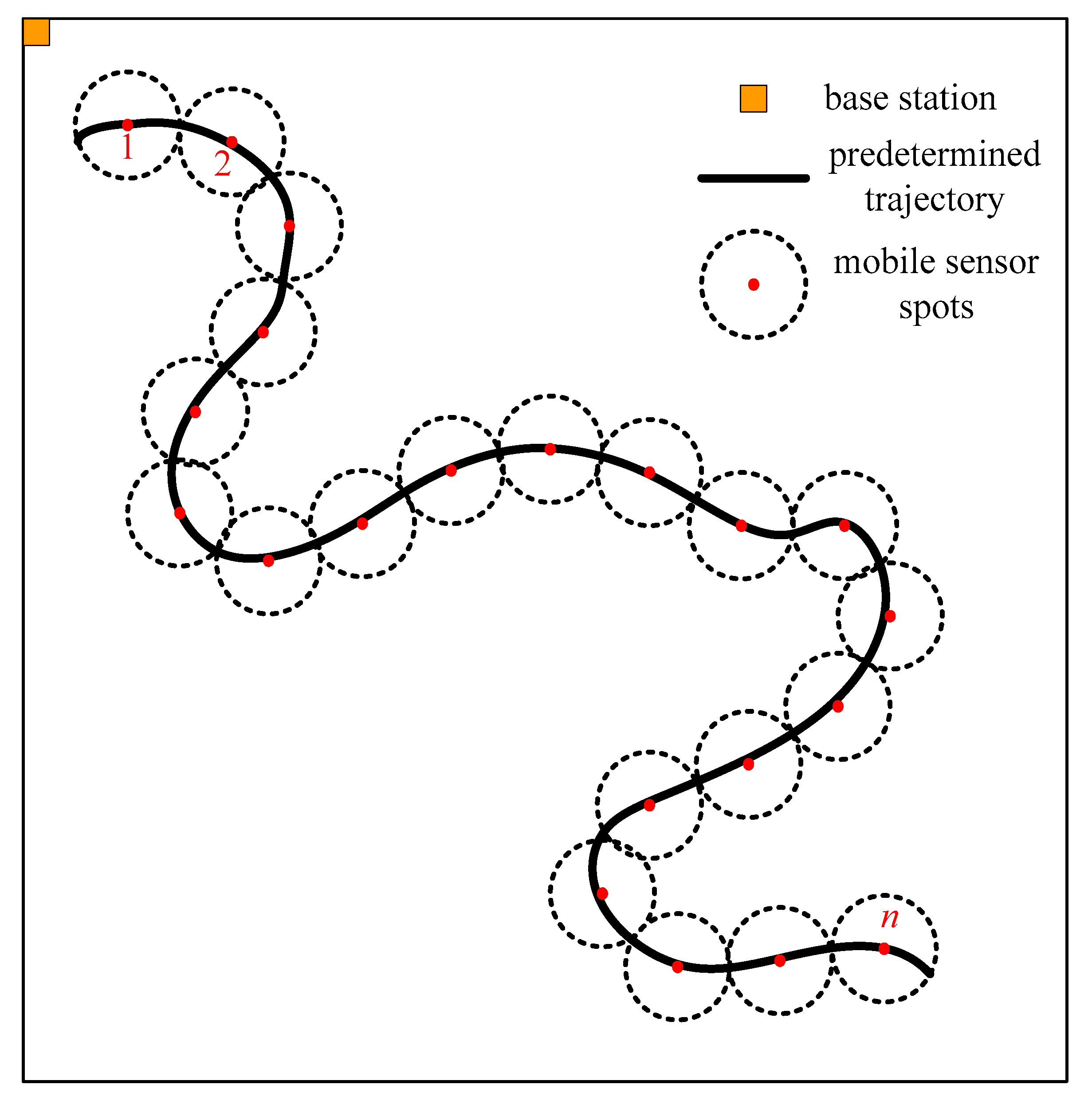
3.1. Network Model and Problem Definition

Consider a WSN model in which an object is planned to travel on a preselected path in a two-dimensional area. To monitor the object, m mobile sensors (e.g., drones) can be used. All the mobile sensors are located in an obstacle-free surveillance region. For convenience, assume that we can schedule mobile sensor nodes to n predetermined spots on the path for monitoring the object before it starts moving (Figure 1). All mobile sensors initially have an equal amount of battery power and are located at the same depot (base station). They also move at the same speed. Each mobile sensor route starts and finishes at the base station. Moreover, a mobile sensor can move to the predetermined position before the object arrives. To extend the network lifetime, we require a movement repertoire of mobile sensors such that the total traveled distance is minimized and as such that the remaining battery power of each sensor is as balanced as possible. We partition the object traveling path into several zones such that each mobile sensor must be placed in a zone once and only once to achieve a high balanced residual energy.

Figure 1. The movement trajectory of an object in the moving object coverage problem.

From a graph-theoretic perspective, the moving object coverage problem can be stated as follows. Let G = (V, A) be a directed multistage graph where V = {0,…, n} is the vertex set, and A is the arc set. The vertices i denote the positions to be reached and monitored, where 1 ≤ i ≤ n, and vertex 0 denotes the base station. The vertices can be partitioned into h ≥ 1 disjoint sets V_i with i = 0,…, h and h = $\frac{n}{m}$, where m > 0 is the number of mobile sensors. Without loss of generality, we assume that n is a multiple of m. The sets of V_i, 0 ≤ i ≤ h, are such that |V₀| = 1 and |V₁| = |V₂|= … = |V_h| = m, where V₀ = {0} and V_i = {(i − 1)$·$m + 1,…, i$·$m}, 1 ≤ i ≤ h. A nonnegative cost d_ij is associated with each arc ⟨i, j⟩ ∈ A, representing the Euclidean distance from vertex i to vertex j. We assume that loops on the same vertex, denoted by d_ii = ∞, where i = 1, 2,…, n, are prohibited. A route is defined as one starting from the base station, going through exactly one vertex in each V_i (where 1 ≤ i ≤ h), and ending at the base station. Each vertex in V_i (where 1 ≤ i ≤ h) must be visited exactly once. Consider a set M = {1, 2,…, m} of identical mobile sensors initially positioned at the base station and are able to move in two dimensions at a constant and homogeneous speed, where 0 < m < n. Each mobile sensor surveils a subset of vertices on the route. The goal is to find a set of routes that can both guarantee that each vertex is served by one mobile sensor and satisfy the constraints of the mobile sensors’ maximum allowable traveled distance. Furthermore, the size of the set should be smaller than the number of mobile sensors required, the total traveled distance should be minimized, and the traveled distance of the mobile sensors should be as balanced as possible. Let $x_{ij}^k$ and $y_i^k$ be binary variables defined as follows:

$$x_{ij}^k=\{\begin{array}{l}1 \mathrm{if} \mathrm{mobile} \mathrm{sensor} k \mathrm{travels} \mathrm{along} \mathrm{arc} ⟨i,j⟩,\\ 0 \mathrm{otherwise}.\end{array}$$

$$y_i^k=\{\begin{array}{l}1 \mathrm{if} \mathrm{mobile} \mathrm{sensor} k \mathrm{reaches} \mathrm{the} \mathrm{spot} i,\\ 0 \mathrm{otherwise}.\end{array}$$

The mathematical formulation of the moving object coverage problem is presented as follows:

$$\min {{\displaystyle \sum }}_{k=1}^m{{\displaystyle \sum }}_{i=0}^n{{\displaystyle \sum }}_{j=0}^n{d}_{ij}{x}_{ij}^k,$$

(1)

$$\min {{\displaystyle \sum }}_{u,v\in M, u\ne v}\left|{{\displaystyle \sum }}_{i=0}^n{{\displaystyle \sum }}_{j=0}^n{d}_{ij}{x}_{ij}^u-{{\displaystyle \sum }}_{i=0}^n{{\displaystyle \sum }}_{j=0}^n{d}_{ij}{x}_{ij}^v \right|$$

(2)

Subject to:

$${{\displaystyle \sum }}_{k=1}^m{y}_i^k=1 \mathrm{for} \mathrm{every} \mathrm{spot} i \in V\backslash \{0\},$$

(3)

$$y_0^k=1 \mathrm{for} \mathrm{every} \mathrm{sensor} k \in M,$$

(4)

where each spot, except the initial base station, must be monitored by exactly one mobile sensor (3) and all mobile sensors must return to the base station (4).

$${{\displaystyle \sum }}_{j=1}^n{x}_{0j}^k=1 \mathrm{for} \mathrm{every} \mathrm{sensor} k \in M,$$

(5)

$${{\displaystyle \sum }}_{i=1}^n{x}_{i0}^k=1 \mathrm{for} \mathrm{every} \mathrm{sensor} k \in M,$$

(6)

where all mobile sensors must start from the base station (5) and stop at the base station (6).

$${{\displaystyle \sum }}_{j=0}^n{{\displaystyle \sum }}_{k=1}^m{x}_{ji}^k=1 \mathrm{for} \mathrm{every} \mathrm{spot} i \in V\backslash \left\{0\right\},$$

(7)

$${{\displaystyle \sum }}_{j=0}^n{{\displaystyle \sum }}_{k=1}^m{x}_{ij}^k=1 \mathrm{for} \mathrm{every} \mathrm{spot} i \in V\backslash \left\{0\right\},$$

(8)

$${{\displaystyle \sum }}_{i=0}^n{x}_{iz}^k-{{\displaystyle \sum }}_{j=0}^n{x}_{zj}^k=0 \mathrm{for} \mathrm{every} \mathrm{spot} z \in V \mathrm{and} \mathrm{for} \mathrm{every} \mathrm{sensor} k \in M,$$

(9)

where each spot must have exactly one incoming and outgoing route [(7)–(9)].

$${{\displaystyle \sum }}_{z=1}^h{x}_{ij}^k=0 \mathrm{for} \mathrm{every} \mathrm{spot} i, j \in V_z \mathrm{and} \mathrm{for} \mathrm{every} \mathrm{sensor} k \in M,$$

(10)

$${{\displaystyle \sum }}_{z=1}^{h-1}{x}_{ij}^k=h-1 \mathrm{for} \mathrm{every} \mathrm{spot} i, j \in V_z \mathrm{and} \mathrm{for} \mathrm{every} \mathrm{sensor} k \in M,$$

(11)

where each mobile sensor cannot travel to the spot in the same subset of its current position (10) and it must travel to one spot in each subset of spots exactly once (11).

$$x_{ii}^k=0 \mathrm{for} \mathrm{every} \mathrm{spot} i, j \in V \mathrm{and} \mathrm{for} \mathrm{every} \mathrm{sensor} k \in M,$$

(12)

where each mobile sensor cannot return to a previously monitored spot.

$$y_i^k \ge x_{ji}^k \mathrm{for} \mathrm{every} \mathrm{spot} i \in V\backslash \left\{0\right\} \mathrm{and} \mathrm{for} \mathrm{every} \mathrm{sensor} k \in M,$$

(13)

$$y_i^k \ge x_{ij}^k \mathrm{for} \mathrm{every} \mathrm{spot} i \in V\backslash \left\{0\right\} \mathrm{and} \mathrm{for} \mathrm{every} \mathrm{sensor} k \in M,$$

(14)

where spot j must be monitored by the mobile sensor that followed the path from spot i to j [(13) and (14)].

The two objective functions [(1) and (2)] represent the total traveled distance to be minimized and the total difference in the distance traveled of all mobile sensors to be minimized, respectively.

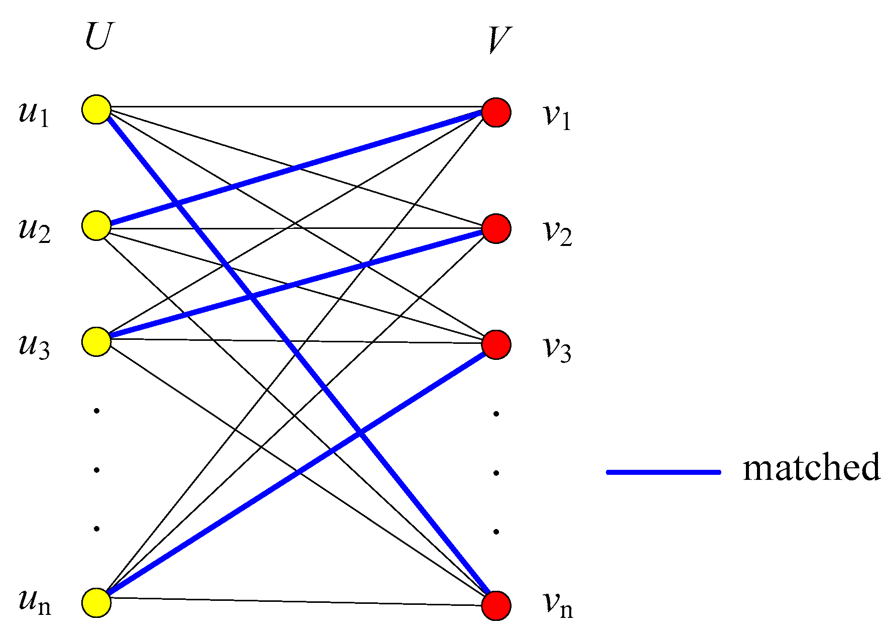
3.2. Greedy Algorithms

The moving object coverage problem is unlikely to be solvable by a brute force approach. Because $\frac{n}{m}$ zones are present and each sensor must move to a unique position in each zone, the total number of feasible movements for m sensors is ${\left(m!\right)}^{\frac{n}{m}-1}$. Therefore, some greedy algorithms are required to solve the moving object coverage problem.

Consider a simple bipartite matching method for mapping sensor positions in two neighboring zones. We generate a weighted complete bipartite graph where a node represents a sensor position and where the weight between two nodes is the distance between sensor positions in neighboring zones (Figure 2). The moving object coverage problem can now be formulated as a sequence of ($\frac{n}{m}$ − 1) complete weighted bipartite graphs, where each set of two consecutive zones, except the base station, forms a complete bipartite graph (Figure 3).

Figure 2. Complete bipartite graph and matching diagram.

Figure 3. Illustration of a sequence of complete bipartite graphs in the moving object coverage problem.

In this paper, we propose distinct greedy algorithms according to weighted bipartite matching methods for the moving object coverage problem under different objective functions. We solve the problem from two perspectives, designated as cases 1 and 2: (1) minimizing the total traveled distance and (2) minimizing the farthest traveled distance of mobile sensors. The proposed greedy solutions are used as bases for comparison. The effects of solving the moving object coverage problem from the two perspectives can be described as follows.

In case 1, the moving object coverage problem can be divided into ($\frac{n}{m}$ − 1) minimum weighted bipartite matching problems on a complete bipartite weighted graph. Given a bipartite graph G = (U, V, E), the minimum weighted bipartite matching problem involves finding a matching in which the sum of the edge weights is minimized. Each minimum weighted bipartite matching problem is clearly independent. Therefore, we can merge the solutions of ($\frac{n}{m}$ − 1) minimum bipartite matching problems to establish the optimal solution for the moving object coverage problem with the goal of minimizing the total traveled distance. We use the Hungarian algorithm [39], a well-known combinatorial optimization method, for solving the weighted bipartite matching problem. Our proposed Algorithm 1 is presented as follows below.

Algorithm 1: Greedy_minimum_weight_matching

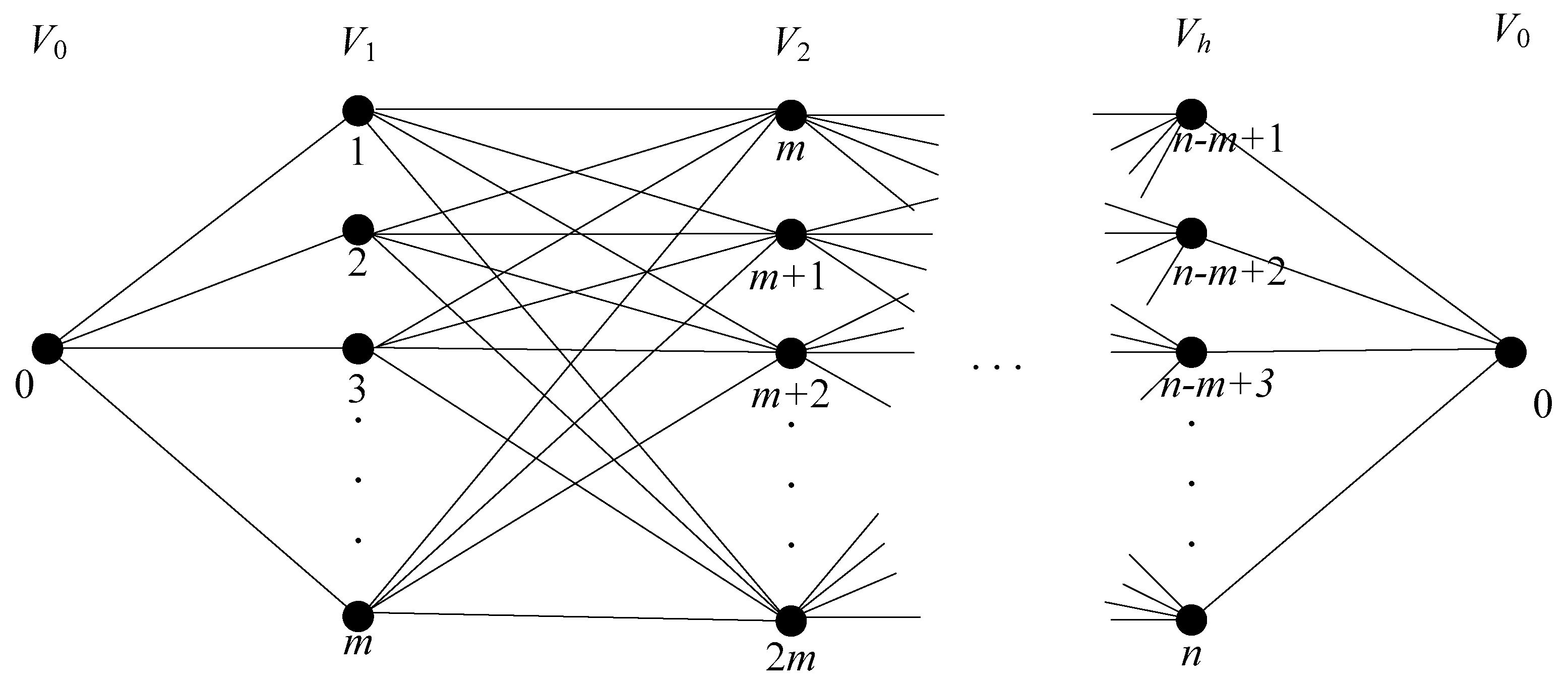
Input: P, m, n  Output: A set M of minimum weight matchings of sensor spots 1: Partition P into $V_1$, $V_2$, …, $V_h$ zones, where h = $\frac{n}{m}$ and $V_i$ = {(i − 1)$·$m + 1, …, i$·$m}, 1 ≤ i ≤ h 2: M = φ 3: i = 1 4:  while i < h do 5:  Construct a weighted complete bipartite graph $G_i$ = ($V_i$, $V_{i+1}$, E), where E refers to the weighted   edges between $V_i$ and $V_{i+1}$. 6:  Find the minimum weight matching $M_i$ of $G_i$ by using the Hungarian method 7:  M = M ∪ $M_i$ 8:  i = i + 1 9: end while 10: return M = {$M_1$, $M_2$, …, $M_{h-1}$}

The time complexity of the greedy minimum weight matching algorithm, designated as Greedy_MWM, is as follows. As noted in [39], the time complexity of the Hungarian method for solving the minimum weighted bipartite matching problem of a weighted complete bipartite graph is O(m³). Therefore, the total time complexity is O(nm²).

In case 2, we solve the moving object coverage problem by solving ($\frac{n}{m}$ − 1) weighted bottleneck bipartite matching problems on a complete weighted bipartite graph. Given a bipartite graph G = (U, V, E), the weighted bottleneck bipartite matching problem entails finding a perfect matching in which the maximum edge weight is minimized. We use the method proposed by Hopcroft and Karp [40] to find this perfect matching in the Euclidean plane. However, the merged solution may not be the optimal solution of the moving object coverage problem—that is, the solution corresponding to the minimum farthest traveled distance. In this paper, we use the merged solution as an approximation solution. Our proposed greedy bottleneck matching Algorithm 2 is presented as follows.

Algorithm 2: Greedy_bottleneck_matching

Input: P, m, n  Output: A set M of bottleneck matchings of sensor positions 1: Partition P into $V_1$, $V_2$, …, $V_h$ zones, where h = $\frac{n}{m}$ and $V_i$ = {(i − 1)$·$m + 1, …, i$·$m}, 1 ≤ i ≤ h 2: M = φ 3: i = 1 4: while i < h do 5:  Construct a weighted complete bipartite graph $G_i$ = ($V_i$, $V_{i+1}$, E), where E represents the weighted    edges between $V_i$ and $V_{i+1}$. 6:  Find the bottleneck matching $M_i$ of $G_i$ by using the Hopcroft–Karp algorithm 7:  M = M ∪ $M_i$ 8:  i = i + 1 9: end while 10: return M = {$M_1$, $M_2$, …, $M_{h-1}$}

As demonstrated in [40], the time complexity associated with the Hopcroft–Karp algorithm for solving the bottleneck matching problem of a weighted complete bipartite graph is O($m^{1.5}\log m$). Therefore, the total time complexity of the greedy bottleneck matching algorithm, designated as Greedy_BM, is O($n\sqrt{m}\log m$).

4. Proposed GA and DPSO Solutions

4.1. GA

A GA is a search algorithm that mimics the evolution of natural organisms. Through genetic manipulation methods, it can create offspring with more favorable solutions. GAs have a widespread application in science, engineering, and business [41,42,43], especially in optimization problems. Its purpose is to find a set of parameters with which the optimal solution to a given problem can be obtained. The main advantage of the GA is that it can achieve a global search effect by using various parameters (e.g., cross-type, population size, and mutation rate) to avoid falling into a state of local optimization.

In general, the use of GAs to solve a specific problem involves four basic steps: problem representation, fitness function, reproduction, and genetic operators. The problem representation refers to the process of translating the phenotype of a problem into a genotype. That is, we encode any element of a candidate solution into the type of a biological gene, and the candidate solution can be represented by a chromosome. Thus, each chromosome is regarded as a point in the space formed by the problem’s solution. The quality of each chromosome can be measured by the fitness function of the problem; in other words, the fitness of the chromosome depends on the extent to which the chromosome can solve the problem. The evolutionary process of GAs can be gradually reproduced through the chromosomes of a population, thereby replacing another population. Genetic operators, such as crossovers and mutations, can be employed to generate better chromosomes in the next generation.

We developed a GA to determine near-optimal or optimal solutions to the moving object coverage problem. The fundamental aspects of the algorithm are described in the following subsections.

4.1.1. Chromosome Representation

Determining the appropriate movement for each mobile sensor is essential for minimizing the traveled distance. Therefore, each chromosome in a population represents a candidate solution to the moving object coverage problem, encoded as the movement of mobile sensors. The length of each chromosome is kept the same as the number of sensor spots. Because the sensor spots are partitioned into zones, we can also partition the chromosome into h = $\frac{n}{m}$ zones, in which each zone consists of m genes. Thus, a possible movement or chromosome can be expressed as:

$$|A_{11} A_{21} ... A_{m1}|A_{12} A_{22} ... A_{m2} | ... |A_{1h} A_{2h} ... A_{mh}|,$$

where $A_{ij}$ ∈ V\{0} represents the location of the sensor spot in the jth zone that is reached by the ith mobile sensor. In this representation, each mobile sensor moves from the sensor spot in the previous zone to the corresponding sensor spot in the next zone. In the following example chromosome,

|1 2 3|4 6 5|7 8 9|,

The movements for mobile sensors in M = {1, 2, 3} are 0 → 1 → 4 → 7 → 0, 0 → 2 → 6 → 8 → 0, and 0 → 3 → 5 → 9 → 0, respectively.

4.1.2. Fitness Evaluation

The proposed chromosome representation is evaluated to find an energy-efficient movement repertoire with a fitness function. To maximize the network lifetime, the evolutionary process of our proposed GA should achieve two objectives: (1) minimizing the total traveled distance of all sensors and (2) optimizing the balance between the residual energy of each sensor. In other words, the first objective involves reducing the total energy consumption, whereas the second objective centers on maximizing the remaining energy of each sensor or controlling the energy consumption of each sensor. These two objectives correspond to the following reasonable considerations. When two movements or chromosomes have the same total distance traveled, a chromosome with a high similarity of residual energy is conducive to network lifetime extension because the remaining energy of each sensor is sufficient to provide full coverage for other moving objects. For the two objectives, we use a fitness function, and the proposed evolutionary algorithm becomes a search for a trajectory that minimizes the fitness function. The fitness value of a trajectory decreases according to the degree to which the objectives are fulfilled. In other words, a trajectory of mobile sensors that fulfills all the objectives well would correspond to a low fitness value. We developed our fitness function to evaluate the fitness of each individual as follows:

$$F=D_c+E_c,$$

where $D_c$ is the cost of the average traveled distance of each sensor and $E_c$ is the cost of the imbalanced energy consumption of each sensor. $D_c$ and $E_c$ can be calculated through the following equations:

$$D_c=\frac{{{\displaystyle \sum }}_{k=1}^m{{\displaystyle \sum }}_{i=0}^n{{\displaystyle \sum }}_{j=0}^n{d}_{ij}{x}_{ij}^k}{m},$$

$$E_c=\frac{ \sigma }{\mu } ·T_d,$$

where $\sigma$ and $\mu$ are the standard deviation and the mean value of the residual energy of all mobile sensors, respectively, and $T_d$ denotes the total distance of the predetermined trajectory.

4.1.3. Selection

We selected candidate individuals from the population in the current generation on the basis of their fitness. Under our proposed GA, roulette wheel selection was employed. Specifically, using a biased roulette wheel, we assigned a slot to each individual; the slot size was proportional to the fitness value of the individual in question. Consequently, individuals with better fitness values were more likely to be selected as individuals in the population of the next generation.

4.1.4. GA Operators

In GAs, the objective of the selection process is to improve the quality of the population, and a new population is generated through crossover and mutation. Therefore, the effectiveness of a GA depends not only on the ability to improve the quality of the population but also on the ability to generate a new population.

Crossover

The crossover operation selects two individuals and subsequently produces two new individuals through an exchange of chromogene parts according to a probability specified by the crossover rate. We used a two-point crossover where two selected individuals exchanged chromogene portions across the boundaries of a segment indicated by two points. The following is an example of a crossover operation:

Indv₁: |1 2 3|6 5 4|9 8 7|

Indv₂: |1 2 3|5 4 6|7 8 9|

After crossover on the second segment, two offspring are created:

Child₁: |1 2 3|5 4 6|9 8 7|

Child₂: |1 2 3|6 5 4|7 8 9|

Mutation

The mutation operator is applied to each zone (except the first zone) of an individual with a probability specified by the mutation rate. When the mutation operator is applied, two sensor spots are randomly selected for a position switch. Figure 4 presents an example of a mutation.

Figure 4. An example of the mutation operation.

4.1.5. Pseudocode of the GA

The pseudocode of our proposed GA for the moving object coverage problem is as follows (Algorithm 3).

Algorithm 3: GA_moving_object_coverage

1: Generate the initial population 2: Evaluate the fitness of each individual in the population 3: while (number of generation < maximum generations) do 4:  while (current crossover queue length < population size) do 5:   Randomly select two different chromosomes C1 and C2 6:   if (C1.fitness > C2.fitness) 7:    Reproduce chromosome C1 to crossover queue 8:   else 9:    Reproduce chromosome C2 to crossover queue 10:   end if 11:  end while 12:  while (current crossover queue is not empty) do 13:   Select and remove two individuals from the queue 14:   Crossover the selected two individuals under a certain probability 15:   Place these two individuals into the new population 16:  end while 17:  for (each individual in the new population) do 18:    Mutating the individual under a certain probability 19:  end for 20:  Evaluate the fitness of each individual in the new population 21:  Set the best fitness value as partial_optimal 21:  Increase number of generation by 1 22: end while 23: global_optimal = partial_optimal 24: return global_optimal

4.2. DPSO Algorithm

Developed by Eberhart and Kennedy in 1995, particle swarm optimization (PSO) is a population-based stochastic optimization technique inspired by the swarming behavior characteristic of bird flocks or fish schools [44]. Similar to the GA, the PSO has recently been applied to combinatorial optimization problems, such as shop scheduling [45,46], the traveling salesman problem [47], Quality of Service multicast routing [48], and vehicle routing [49,50]. The PSO algorithm, which is based on a metaphor of social interaction, searches a space by adjusting the trajectories of individual vectors called ‘particles, which are conceptualized as moving points in a multidimensional space. Individual particles are drawn stochastically toward the position of their own best previous performance and the best global performance among their neighbors. The PSO algorithm is simple, easy to implement, robust for parameter control, and computationally efficient compared with other heuristic optimization techniques. The original PSO has been applied to learning problems involving neural networks as well as to function optimization problems, and its efficiency has been confirmed.

When used to solve an optimization problem, the PSO algorithm simulates the movement of a swarm of particles in a multidimensional search space, progressing toward an optimal solution. The position of each particle represents a candidate solution and is randomly initiated. In our implementation, the position of a particle represents a complete trajectory with the same encoding as that under the GA. At each iteration, the fitness function is evaluated for each particle in the swarm and is compared with (1) the fitness of the best previous result for that particle and (2) the fitness of the best particle among all particles in the swarm. After the two best values are found, the particles evolve by updating their velocities and positions according to the following equations:

$$V_i^{t+1}=\omega \ast V_i^t+c_1\ast r_1\ast \left(P_i^t-X_i^t\right)+c_2\ast r_2\ast \left(G^t-X_i^t\right)$$

(15)

$$X_i^{t+1}=X_i^t+V_i^{t+1}$$

(16)

where i = (1, 2,…, P) and P is the size of the swarm; $X_i^t$ and $V_i^t$ are the position and velocity of the ith particle at iteration t, respectively; ω is the inertia weight, a parameter controlling the impact of the previous velocities on the current velocity; $P_i^t$ is the best-reached solution on the particle scale; and $G^t$ is the global best solution in the swarm. Here, $c_1$ and $c_2$ are acceleration coefficients and $r_1$ and $r_2$ denote uniform random numbers between (0, 1). The recursive steps continue until the termination condition is reached.

4.2.1. DPSO Approach

Given that particle positions are real-valued, standard PSO equations clearly cannot be used to generate the solution of a discrete optimization problem. Therefore, we must modify the position and velocity vector represented in (15) and (16) in the original PSO algorithm such that it spans the discrete search domain. For our moving object coverage problem, we develop a DPSO algorithm that is an adaptation of the method established in [45] to update particle positions. According to [45], the position of the ith particle at iteration t can be updated as follows:

$$X_i^{t+1}=c_2 \oplus F_3\left(c_1 \oplus F_2\left(\omega \oplus F_1\left(X_i^t\right), P_i^t\right), G^t\right)$$

(17)

where $F_1$, $F_2$, and $F_3$ are operations with the probabilities $\omega$, $c_1$, and $c_2$, respectively.

Given that ${\tau }_i^{t+1}$ and ${\delta }_i^{t+1}$ are temporary individuals, in the DPSO algorithm, the update equation consists of three components, and the particle velocities and positions are updated by using the following operations:

• The first component is ${\tau }_i^{t+1}=\omega \oplus F_1\left(X_i^t\right)$, which represents the velocity of the particle. $F_1$ denotes the mutation operator, which corresponds to a probability of $\omega .$ In other words, a uniform random number r is generated between 0 and 1. If r is less than $\omega$, the mutation operator is applied to generate a possible new particle by ${\tau }_i^{t+1}=F_1\left(X_i^t\right)$. Otherwise, the current particle is kept as ${\tau }_i^{t+1}=X_i^t.$

• The second component is ${\delta }_i^{t+1}=c_1 \oplus F_2\left({\tau }_i^{t+1}, P_i^t\right),$ the “cognitive” part of the particle; that is, it represents the individual-level thinking of the particle. $F_2$ represents the crossover operator, which corresponds to a probability of $c_1.$ Depending on the choice of a uniform random number, the outcome is either ${\delta }_i^{t+1}=F_2\left({\tau }_i^{t+1}, P_i^t\right)$ or ${\delta }_i^{t+1}={\tau }_i^{t+1}$.

• The third component, $X_i^{t+1}=c_2 \oplus F_3\left({\delta }_i^{t+1}, G^t\right),$ is the “social” part of the particle, representing interparticle collaboration. $F_3$ denotes the crossover operator, which corresponds to a probability of $c_2.$ Depending on the choice of a uniform random number, the outcome is either $X_i^{t+1}=F_3\left({\delta }_i^{t+1}, G^t\right)$ or $X_i^{t+1}={\delta }_i^{t+1}$.

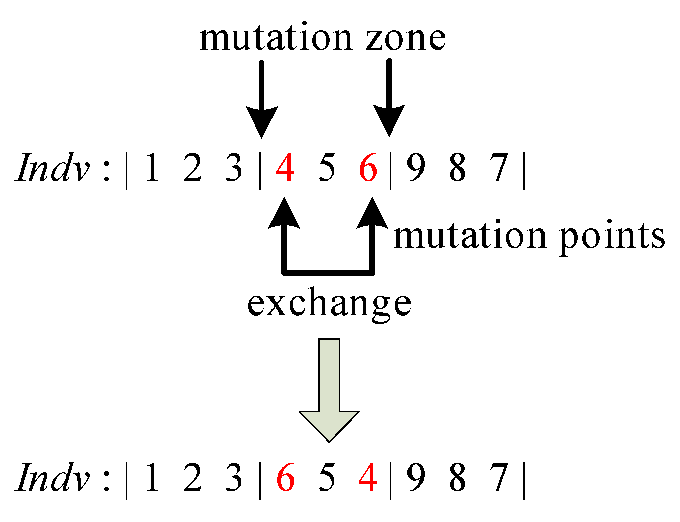
• The mutation operator $F_1$ on a position $X_i^t$ is defined as the exchange of two randomly selected sensor spots in a randomly selected zone. For example, with $X_i^t$ = |1 2 3|4 5 6|7 8 9| and the mutation point being the first and second positions in zone 3, by applying the mutation operator, we obtain ${\tau }_i^{t+1}$ = |1 2 3|4 5 6|8 7 9|.

• The crossover operator $F_2$ is defined as taking ${\tau }_i^{t+1}$ and $P_i^t$ as the first and second parents as the crossover operator, respectively. When the crossover operator is applied, each of the different sensor spots in ${\tau }_i^{t+1}$ and $P_i^t$, from left to right, is taken to be exchanged if a uniform random number r ∈ (0, 1) is generated and if r < $c_1$. For example, with ${\tau }_i^{t+1}$ = |1 2 3|5 4 6|9 7 8| and $P_i^t$ = |1 2 3|5 4 6|9 8 7|, we obtain ${\delta }_i^{t+1}$ = |1 2 3|5 4 6|9 8 7| if both generated uniform random numbers are less than $c_1$. The exchanged result must be a legal solution; therefore, some adjustments must be made. In our implementation, if ${\delta }_i^{t+1}$ = |1 2 3|5 4 6|9 8 8| after the exchange of ${\tau }_i^{t+1}$ and $P_i^t$ on the second position in zone 3, we adjust the third position in zone 3 from 8 to 7 to ensure its legality as a solution.

• The crossover operator $F_3$ is defined as the taking of ${\delta }_i^{t+1}$ and $G^t$ as the first and second parent for the crossover operator, respectively. When the crossover operator is applied, similar to the operation in $F_2$, each of the sensor spots in ${\delta }_i^{t+1}$ and $G^t$ is taken, from left to right, to be exchanged if a uniform random number r ∈ (0, 1) is generated and if r < $c_2$.

We followed the gbest model developed by Kennedy et al. [44] in implementing our DPSO algorithm. Under the same encoding as that used under the GA, the position of a particle represents a complete trajectory. Here, we employ the same fitness function as that employed under the GA.

4.2.2. Pseudocode of the DPSO Algorithm

The pseudocode of our DPSO Algorithm 4 for the moving object coverage problem is listed as follows.

Algorithm 4: DPSO_moving_object_coverage

1: Initialize the parameters of DPSO. Set the swarm size and generate the initial particles with position and velocity, and set the generation counter to 1. 2: for (each particle in the swarm) do 3:   Compute the fitness value of each particle 4:   Set the particle_best value of each particle to itself 5: end for 6: Set global_best value to the best fit particle 7: while (number of generation < maximum generations) do 8:   for (each particle in the swarm) do 9:    Compute the new velocity and new position by using the mutation operator $F_1$ and crossover operators $F_2$ and $F_3$ in (17) under a certain probability 10:    Update fitness of new position 11:    if (new fitness < particle_best) 12:     particle_best = new fitness 13:    end if 14:  end for 15:  Find the particle with the best fitness and update global_best 16:  Increase the number of generation by 1 17: end while 18: return global_best

5. Performance Evaluation and Comparison

We compared the results obtained using the greedy algorithms (Greedy_MWM and Greedy_BM) with those obtained using the GA and DPSO algorithm in a set of simulation experiments. All experiments were performed using a program in C# on a NET platform. Specifically, the simulation was conducted using 40 distinct trajectories for each number of sensor spots, and each trajectory was applied 50 times. The recorded data were averaged to generate the final results. Table 1 presents the parameter settings in our simulations.

Table 1. Parameter settings in the simulations.

Parameter	Value	Meaning
AM	1000 m × 1000 m	Network monitoring area
r	25 m	Sensors’ coverage radius
(x0, y0)	(0, 0)	Base station location
n	20, 30,…, 100	Number of sensor spots
m	5	Number of mobile sensors
P	100	Population size
Pc	0.8	Probability of crossover (GA only)
Pm	0.1	Probability of mutation (GA only)
$\omega$	0.1	Probability of mutation (DPSO only)
$c_1$	0.5	Probability of crossover (DPSO only)
$c_2$	0.5	Probability of crossover (DPSO only)
Ic	100, 1000	Number of generations (GA) or iterations (DPSO)

Our simulations focused on determining algorithm performance regarding the effect of the number of sensor spots on the total energy consumption, the balance of the residual energy of all sensors, and the quality of the solutions. In terms of total energy consumption, system efficiency was evaluated according to the sensors’ total traveled distance. Regarding the balance of residual energy, system efficiency was assessed by the differences in the distance traveled of all mobile sensors. Solution quality (and by extension, algorithm quality) was indicated by the fitness value.

Figure 5 presents the effect of the number of sensor spots on the total traveled distance under the GA and DPSO algorithm, compared to the solutions obtained by the greedy algorithms. In terms of the total traveled distance, the greedy minimum weight matching algorithm performed the best regardless of the number of sensor spots, whereas the greedy bottleneck matching algorithm performed the worst. The DPSO approach performed slightly better than did the GA approach given the small number of sensor spots. However, as the number of sensor spots increased, the GA approach outperformed the DPSO approach by 0.1% to 0.3% in terms of the total traveled distance. This is attributable to the small number of sensor spots, to which the presence of many similar individuals in each population is ascribable. Therefore, the GA approach is more likely to approach a local optimum than is the DPSO approach. As the size of the problem increased, the GA saved the better results from the previous generation and passed them to the next generation through an evolutionary process. By contrast, under the DPSO approach, the better results in each generation did not always have the chance to improve the outcomes of each particle. Consequently, the GA approach was more likely to approach the global optimum through the evolutionary process.

Figure 5. Total traveled distance under the greedy algorithms, genetic algorithm (GA), and discrete particle swarm optimization (DPSO) algorithm.

Figure 6 presents the effect of the number of sensor spots on the differences in the mobile sensors’ residual energy under the greedy algorithms, GA, and DPSO algorithm. In terms of the total differences in the distance traveled by mobile sensors, the greedy approaches were considerably outperformed by the evolutionary schemes; their outcomes ranged from 33% worse to 53 times worse than those of the GA and DPSO algorithms. The GA approach outperformed the DPSO approach in terms of the balance of residual energy, regardless of the number of sensor spots. As the number of sensor spots increased, the difference between the performance of the GA and DPSO approaches increased from 2.1% to 77%. This is attributable to the small number of sensor spots, to which the presence of many similar individuals in each population is ascribable. Therefore, the GA approach is more likely to approach a local optimum than is the DPSO approach. As the size of the problem increased, the GA saved the better results from the previous generation and passed them to the next generation through an evolutionary process. By contrast, under the DPSO approach, the better results in each generation did not always have the chance to improve the outcomes of each particle. Consequently, the GA approach is more likely to approach the global optimum through the evolutionary process.

Figure 6. Differences in the total traveled distance under the greedy algorithms, GA, and DPSO algorithm.

Figure 7 displays the effect of the number of sensor spots on the quality of solutions generated by the greedy algorithms, the GA, and the DPSO algorithm. The fitness values obtained by the greedy algorithms were approximately 2.2% worse than were those obtained by the evolutionary algorithms. Regardless of the number of sensor spots, the GA had better fitness values than the DPSO algorithm (a difference of 0.14% to 0.43%). In short, the GA outperformed the DPSO algorithm according to the fitness function. Moreover, the GA approach was more likely to approach the global optimum than was the DPSO approach through evolutionary generation.

Figure 7. Fitness values of the greedy algorithms, GA, and DPSO algorithm.

Figure 8 illustrates the effect of the number of evolutionary generations on the fitness function under the GA and DPSO schemes when n = 60, m = 5, and I_c = 100. With respect to the fitness values, the GA approach outperformed the DPSO approach after 15 generations and achieved solutions that were 0.3% better.

Figure 8. Fitness values of the GA and DPSO algorithm in 100 generations when n = 60 and m = 5.

We continued the preceding experiment, extending the number of iterations from 100 to 1000 to investigate the performance of the proposed GA and DPSO approaches. Figure 9 presents the experimental results obtained when n = 60, m = 5, and I_c = 1000. As the number of iterations increased, the fitness improved correspondingly, and after 300 generations, the GA had approached a convergent solution. Notably, the DPSO algorithm obtained a near-convergent solution after 150 generations.

Figure 9. Fitness values of the GA and DPSO algorithm achieve over 1000 generations when n = 60.

Figure 10 presents the effect of the number of sensor spots on the average running time required by the greedy algorithms, the GA, and the DPSO algorithm. The running time required by the greedy algorithms was less than 50 milliseconds, which is much less than that required by the meta-heuristic algorithms. Regardless of the number of sensor spots, the GA required considerably (approximately 4.8–10 times) more running time than did the DPSO algorithm. In short, the DPSO algorithm outperformed the GA with regard to average running time; therefore, the DPSO approach was more efficient in approaching the global optimum through evolutionary generation than was the GA approach.

Figure 10. Average running time of the greedy algorithms, GA, and DPSO algorithm.

In the simulations, we further compared the performance of the GA and the DPSO algorithm (in terms of the average traveled distance, the average difference in the distance traveled, and average fitness values) by considering 40 distinct, randomly generated scenarios. Table 2 displays the average traveled distance of the 50 trajectories generated under a population size of 100 when n = 40 and m = 5. To compare our implementation of the GA and the DPSO algorithm, we conducted a t-test [51] of the cost distribution of the trajectories obtained by each algorithm. In Table 2, the p-value obtained in the t-test represents the probability that the difference between the two averages is due to chance. In other words, when the p-value obtained is <0.05, the two averages differ significantly, and the probability that this difference is not due to chance is 95%. Comparing the averages presented in Table 2 (note that an X indicates the winner of the performance comparison of each scenario), we observed the following:

Table 2. Average traveled distance of the 50 trajectories generated for each of the 40 scenarios using the GA and DPSO algorithm when n = 40 and m = 5.

Scenario	Average Traveled Distance and Standard Deviation of Generated Trajectories (50 Trials)		p-Value (Test-T)	Average Are Statistically Different	Winner
	GA	DPSO			GA	PSO
1	2992.4393 ± 1.8196	2992.9436 ± 3.6418	0.381	no
2	3128.3941 ± 2.0386	3129.8614 ± 2.7980	0.005	yes	X
3	3209.4913 ± 1.0822	3207.5020 ± 2.0464	0.000	yes		X
4	3220.0346 ± 0.9116	3219.3740 ± 2.2181	0.049	yes		X
5	2856.9409 ± 3.8808	2854.5864 ± 5.4068	0.011	yes		X
6	3014.5629 ± 3.0619	3011.0986 ± 4.2573	0.000	yes		X
7	3001.8451 ± 3.4108	3002.7971 ± 3.7244	0.210	no
8	2991.8435 ± 1.5807	2990.9248 ± 2.5517	0.034	yes		X
9	2902.0144 ± 2.6819	2899.2818 ± 3.7795	0.000	yes		X
10	2989.3441 ± 1.7431	2988.9386 ± 2.7793	0.383	no
11	3058.3370 ± 1.3551	3057.3041 ± 2.9977	0.009	yes		X
12	3030.9654 ± 0.5501	3027.7668 ± 3.4714	0.000	yes		X
13	3010.7018 ± 1.2675	3008.8785 ± 2.7130	0.000	yes		X
14	2812.4526 ± 2.9295	2807.2978 ± 4.4937	0.000	yes		X
15	3003.6262 ± 3.5982	2999.7705 ± 4.8891	0.011	yes		X
16	3053.5578 ± 1.4282	3054.4615 ± 2.9521	0.088	no
17	3008.8329 ± 1.6307	3005.3759 ± 3.9018	0.000	yes		X
18	2622.5295 ± 6.0524	2628.4946 ± 7.1286	0.000	yes	X
19	3081.6292 ± 2.5140	3085.4334 ± 4.9469	0.000	yes	X
20	3250.4881 ± 2.2775	3248.7471 ± 2.5949	0.002	yes		X
21	2972.0539 ± 3.0167	2972.9801 ± 3.3745	0.158	no
22	2973.8529 ± 2.1972	2973.3860 ± 2.8221	0.374	no
23	2874.8155 ± 2.4585	2870.9051 ± 4.1883	0.000	yes		X
24	3100.4265 ± 1.6634	3101.8846 ± 4.0950	0.033	yes	X
25	2977.7085 ± 3.4182	2978.8530 ± 4.6732	0.187	no
26	2900.0235 ± 1.9922	2901.5632 ± 3.4843	0.008	yes	X
27	3045.3884 ± 2.1302	3045.2916 ± 2.9441	0.833	no
28	3157.2719 ± 1.1186	3156.7508 ± 2.8880	0.242	no
29	3019.8295 ± 1.7735	3020.7697 ± 3.2370	0.093	no
30	2797.1633 ± 3.3278	2796.4397 ± 6.5181	0.479	no
31	3010.7305 ± 1.7398	3013.0609 ± 3.4161	0.000	yes	X
32	2995.7100 ± 2.1156	2993.5887 ± 4.9071	0.005	yes		X
33	2774.9727 ± 2.1628	2776.1326 ± 5.0659	0.164	no
34	2868.4977 ± 2.5431	2864.9081 ± 5.0707	0.000	yes		X
35	2917.6947 ± 4.3329	2919.3911 ± 5.5848	0.115	no
36	2974.5797 ± 2.9380	2971.5000 ± 4.3944	0.000	yes		X
37	2974.2939 ± 3.3901	2975.9473 ± 5.2312	0.056	no
38	3057.1951 ± 1.6681	3058.3120 ± 2.6079	0.018	yes	X
39	2856.6309 ± 2.9443	2852.8555 ± 3.4337	0.000	yes		X
40	2973.7681 ± 3.8462	2971.8546 ± 6.2907	0.077	no
			Total	15/40	7/40	18/40

• The GA generated better trajectories than the DPSO algorithm in 7 of the 40 scenarios;
• The DPSO algorithm generated significantly better trajectories than the GA in 18 of the 40 scenarios;
• The GA and DPSO generated similarly performing trajectories in 15 of the 40 scenarios.

On the basis of these results, we conclude that the DPSO algorithm outperforms the GA in solving the moving object coverage problem when n = 40 and m = 5. However, as mentioned, the GA outperformed the DPSO algorithm when the problem scale increased. Table 3, Table 4 and Table 5 present the average traveled distance, the average difference in the distance traveled, and average fitness values obtained using the GA and DPSO algorithm for different problem scales, respectively. From these results, we conclude that:

Table 3. Average traveled distance under the GA and DPSO algorithm.

Problem Scales	Similar Quality	GA Wins	DPSO Wins
20	23	4	13
30	15	5	20
40	15	7	18
50	13	11	16
60	10	15	15
70	10	29	1
80	5	31	4
90	0	40	0
100	0	40	0

Table 4. Average difference in the distance traveled under the GA and DPSO algorithm.

Problem Scales	Similar Quality	GA Wins	DPSO Wins
20	0	40	0
30	0	40	0
40	0	40	0
50	0	40	0
60	0	40	0
70	0	40	0
80	0	40	0
90	0	40	0
100	0	40	0

Table 5. Average fitness values of the GA and DPSO algorithm.

Problem Scales	Similar Quality	GA Wins	DPSO Wins
20	0	40	0
30	0	40	0
40	0	40	0
50	0	40	0
60	0	40	0
70	0	40	0
80	0	40	0
90	0	40	0
100	0	40	0

• The GA generated better trajectories than the DPSO algorithm in terms of average traveled distance as the problem scale increased;
• The GA generated significantly better trajectories than the DPSO algorithm in terms of the average difference in the distance traveled, regardless of the problem scale;
• The GA generated significantly better trajectories than the DPSO algorithm in terms of average fitness values, regardless of the problem scale.

In summary, the GA approach is preferable to the DPSO approach for solving the moving object coverage problem.

6. Discussion

In this paper, we propose two meta-heuristic algorithms to solve the moving object coverage problem and compare their performance in terms of solution optimality and system running time. Because of the increasing use of mobile sensors, their applications in traditional WSNs, such as target tracking and moving object coverage, have become broader and more practical. The key factors in designing an energy-efficient mobile WSN for a specific purpose include residual energy utilization, mobility, topology, scalability, localization, data collection routing, and quality of service. Therefore, the effective management of the energy consumption of mobile sensors is a crucial research topic, and this paper contributes to the body of literature on this topic by proposing algorithms that can be used to achieve energy-saving mobility.

Although the research has proposed two meta-heuristic algorithms for resolving the moving object coverage problem effectively, it still has the following limitations: (1) We only take into account the moving distance as the main factor of energy consumption of mobile sensors; (2) we partition the sensor spots into several small zones to simplify the complexity of the problem; (3) we assume that all mobile sensors are identical, which means that the battery energy drain can be identical to each mobile sensor; (4) the experiment only considers the randomly generated trajectories. In real-world applications, the moving trajectory may be specific paths; the proposed meta-heuristic algorithms have disadvantages, such as the computational expensiveness of the GA, the premature convergence in the DPSO algorithm, and no guarantees for achieving the optimal solutions.

Despite the aforementioned limitations, the experimental results show that they are still more suitable than traditional heuristic algorithms for solving complex optimization problems, such as the moving object coverage problem.

Our analyses revealed that the GA outperformed the DPSO algorithm in all the evaluation metrics, especially in solving large problems. However, the GA required more running time than did the DPSO algorithm. This is because the operations involved in the GA are mainly selection, crossover, and mutation. Because selection involves identifying and retaining higher-quality chromosomes for the next generation, the GA requires more computation time but obtains more accurate solutions than does the DPSO algorithm. Conversely, the advantage of DPSO is its simplicity, which results in rapid convergence. To overcome the limitations and draw on the advantages of both algorithms, a combination of the algorithms can be used. Fusing these two algorithms together results in the creation of a composite algorithm with practical value and high performance. Therefore, a hybrid of the GA and DPSO algorithms should be explored in future research.

Finally, despite studies commonly reporting that most energy consumption by mobile sensors is caused by the movement of the sensors and is related to the distance traveled, this explanation is not practical in some situations. For example, when a small drone is used as a mobile platform to carry sensors, the energy consumption will also vary according to weather conditions, changes in the communication environment, or flight altitudes. Therefore, additional factors that may affect energy consumption must be considered in practical applications.

7. Conclusions and Future Work

We considered the moving object coverage problem in a WSN with a limited number of mobile sensors. We required full coverage of a moving object on a predetermined trajectory. To conserve energy, we determined a movement repertoire where the total traveled distance was minimized and where the residual energy of the mobile sensors was as balanced as possible. Our results revealed that a very long time is required to determine the optimal solution to the moving object coverage problem when the predetermined trajectory is expansive. We employed two nondeterministic algorithms, the GA, and the DPSO algorithm, to manage this complexity and produce solutions at a relatively short computation time. The algorithms generated effective solutions to the moving object coverage problem efficiently. Our algorithms quickly determined quasi-optimal trajectories for mobile sensors and were determined to be applicable to larger predetermined trajectories. Under the same encoding, the GA produced trajectories significantly superior to those produced by the DPSO algorithm.

In the future, the proposed algorithms can be applied to tracking multiple objects in the same area, each with a different predetermined path. Developing a hybrid of the GA and DPSO algorithms for moving object coverage problems may also be an area of interest. It is also interesting to study specific trajectories, such as the Hilbert space-filling curve. Furthermore, regarding the practical applications of sensors, future studies should evaluate the effects of different environmental parameters, such as wind speed, altitude, flying speed, and changes in the communication environment.

References

- Yick, J.; Mukherjee, B.; Ghosal, D. Wireless sensor network survey. Comput. Netw. 2008, 52, 2292–2330. [Google Scholar] [CrossRef]
- Kulaib, A.R.; Shubair, R.M.; Al-Qutayri, M.A.; Ng, J.W.P. An overview of localization techniques for wireless sensor networks. In Proceedings of the International Conference on Innovations in Information Technology, Abu Dhabi, United Arab Emirates, 25–27 April 2011; pp. 167–172. [Google Scholar] [CrossRef]
- Sibley, G.T.; Rahimi, M.H.; Sukhatme, G.S. Robomote: A tiny mobile robot platform for large-scale sensor networks. In Proceedings of the IEEE International Conference on Robotics and Automation, Washington, DC, USA, 11–15 May 2002; pp. 1143–1148. [Google Scholar] [CrossRef]
- Liang, C.K.; Lin, Y.H. A coverage optimization strategy for mobile wireless sensor networks based on genetic algorithm. In Proceedings of the IEEE International Conference on Applied System Invention (ICASI), Chiba, Japan, 13–17 April 2018; pp. 1272–1275. [Google Scholar] [CrossRef]
- Aslam, J.; Butler, Z.; Constantin, F.; Crespi, V.; Cybenko, G.; Rus, D. Tracking a moving object with a binary sensor network. In Proceedings of the International Conference on Embedded networked sensor systems, Dana Point, CA, USA, 20–21 October 2003; pp. 150–161. [Google Scholar] [CrossRef]
- Kung, H.T.; Vlah, D. Efficient location tracking using sensor networks. In Proceedings of the IEEE Wireless Communications and Networking Conference (WCNC), New Orleans, LA, USA, 16–20 March 2003. [Google Scholar] [CrossRef]
- Zhang, W.; Cao, G. DCTC: Dynamic convoy tree-based collaboration for target tracking in sensor networks. IEEE Trans. Wireless Commun. 2004, 3, 1689–1701. [Google Scholar] [CrossRef] [Green Version]
- Jin, G.Y.; Lu, X.Y.; Park, M.S. Dynamic clustering for object tracking in wireless sensor networks. In Proceedings of the International Symposium on Ubiquitous Computing Systems, Seoul, Korea, 11–13 October 2006; pp. 200–209. [Google Scholar] [CrossRef]
- Souza, E.L.; Nakamura, E.F.; Pazzi, R.W. Target tracking for sensor networks: A survey. ACM Comput. Surv. 2017, 49, 1–31. [Google Scholar] [CrossRef]
- Leela Rani, P.; Sathish Kumar, G.A. Detecting Anonymous Target and Predicting Target Trajectories in Wireless Sensor Networks. Symmetry 2021, 13, 719. [Google Scholar] [CrossRef]
- Manjeshwar, A.; Agrawal, D.P. APTEEN: A hybrid protocol for efficient routing and comprehensive information retrieval in wireless sensor networks. In Proceedings of the International Parallel and Distributed Processing Symposium, Lauderdale, FL, USA, 15–19 April 2002; pp. 195–202. [Google Scholar] [CrossRef]
- Chen, T.S.; Chen, J.J.; Wu, C.H. Distributed object tracking using moving trajectories in wireless sensor networks. Wirel. Netw. 2016, 22, 2415–2437. [Google Scholar] [CrossRef]
- Lin, K.W.; Hsieh, M.H.; Tseng, V.S. A novel prediction based strategy for object tracking in sensor networks by mining seamless temporal movement patterns. Expert Syst. Appl. 2010, 37, 2799–2807. [Google Scholar] [CrossRef]
- Yu, X.; Liang, J. Genetic fuzzy tree based node moving strategy of target tracking in multimodal wireless sensor networks. IEEE Access 2018, 6, 25764–25772. [Google Scholar] [CrossRef]
- Liu, B.; Dousse, O.; Nain, P.; Towsley, D. Dynamic Coverage of Mobile Sensor Networks. IEEE Trans. Parallel Distrib. Syst. 2013, 24, 301–311. [Google Scholar] [CrossRef] [Green Version]
- Burgos, U.; Amozarrain, U.; Gomez-Calzado, C.; Lafuente, A. Routing in Mobile Wireless Sensor Networks: A Leader-Based Approach. Sensors 2017, 17, 1587. [Google Scholar] [CrossRef] [Green Version]
- Nguyen, N.T.; Liu, B.H. The mobile sensor deployment problem and the target coverage problem in mobile wireless sensor networks are NP-hard. IEEE Syst. J. 2019, 13, 1312–1315. [Google Scholar] [CrossRef]
- De Freitas, E.P.; Heimfarth, T.; Netto, I.F.; Lino, C.E.; Pereira, C.E.; Ferreira, A.M.; Wagner, F.R.; Freitas, L.T. UAV relay network to support WSN connectivity. In Proceedings of the International Congress on Ultra Modern Telecommunications and Control Systems (ICUMT), Moscow, Russia, 18–20 October 2010; pp. 309–314. [Google Scholar] [CrossRef]
- Heinzelman, W.B.; Chandrakasan, A.P.; Balakrishnan, H. An application-specific protocol architecture for wireless microsensor networks. IEEE Trans. Wirel. Commun. 2002, 1, 660–670. [Google Scholar] [CrossRef] [Green Version]
- Oliveira, H.A.; Barreto, R.S.; Fontao, A.L.; Loureiro, A.A.; Nakamura, E.F. A novel greedy forward algorithm for routing data toward a high speed sink in wireless sensor networks. In Proceedings of the 19th International Conference on Computer Communications and Networks (ICCCN), Zurich, Switzerland, 2–5 August 2010; pp. 1–7. [Google Scholar] [CrossRef]
- Jawhar, I.; Mohamed, N.; Al-Jaroodi, J.; Zhang, S. A framework for using unmanned aerial vehicles for data collection in linear wireless sensor networks. J. Intell. Rob. Syst. 2014, 74, 437–453. [Google Scholar] [CrossRef]
- Ali, Z.A.; Masroor, S.; Aamir, M. UAV based data gathering in wireless sensor networks. Wireless Pers. Commun. 2019, 106, 1801–1811. [Google Scholar] [CrossRef]
- Daponte, P.; Vitto, L.D.; Mazzilli, G.; Picariello, F.; Rapuano, S.; Riccio, M. Metrology for drone and drone for metrology: Measurement systems on small civilian drones. In Proceedings of the 2015 IEEE Metrology for Aerospace (MetroAeroSpace), Benevento, Italy, 4–5 June 2015; pp. 306–311. [Google Scholar] [CrossRef]
- Flammini, F.; Pragliola, C.; Smarra, G.; Naddei, R. Towards automated drone surveillance in railways: State-of-the-art and future directions. In Proceedings of the International Conference on Advanced Concepts for Intelligent Vision Systems (ACIVS), Lecce, Italy, 24–27 October 2016; pp. 336–348. [Google Scholar] [CrossRef]
- Hu, Z.; Gu, D.; Song, Z.; Li, H. Localization in wireless sensor networks using a mobile anchor node. In Proceedings of the IEEE/ASME International Conference on Advanced Intelligent Mechatronics, Xi’an, China, 2–5 July 2008; pp. 602–607. [Google Scholar] [CrossRef]
- Huang, K.F.; Chen, P.J.; Jou, E. Grid-based localization mechanism with mobile reference node in wireless sensor networks. J. Electron. Sci. Technol. 2014, 12, 283–287. [Google Scholar] [CrossRef]
- Farmani, M.; Moradi, H.; Dehghan, S.M. The modified Hilbert path for mobile-beacon-based localization in wireless sensor networks. Trans. Inst. Meas. Control 2013, 36, 916–923. [Google Scholar] [CrossRef]
- Rezazadeh, J.; Moradi, M.; Ismail, A.S. Superior path planning mechanism for mobile beacon-assisted localization in wireless sensor networks. IEEE Sens. J. 2014, 14, 3052–3064. [Google Scholar] [CrossRef]
- Chen, Y.; Lu, S.; Chen, J.; Ren, T. Node localization algorithm of wireless sensor networks with mobile beacon node. Peer-to-Peer Netw. Appl. 2017, 10, 795–807. [Google Scholar] [CrossRef]
- Alomari, A.; Phillips, W.; Aslam, N.; Comeau, F. Swarm intelligence optimization techniques for obstacle-avoidance mobility-assisted localization in wireless sensor networks. IEEE Access 2018, 6, 22368–22385. [Google Scholar] [CrossRef]
- Li, Z.; Lei, L. Sensor node deployment in wireless sensor networks based on improved particle swarm optimization. In Proceedings of the International Conference on Applied Superconductivity and Electromagnetic Devices (ASEMD), Chengdu, China, 25–27 September 2009; pp. 215–217. [Google Scholar] [CrossRef]
- Peiravi, A.; Mashhadi, H.R.; Javadi, S.H. An optimal energy-efficient clustering method in wireless sensor networks using multi-objective genetic algorithm. Int. J. Commun. Syst. 2013, 26, 114–126. [Google Scholar] [CrossRef]
- Zungeru, A.M.; Seng, K.P.; Ang, L.M.; Conge Chia, W. Energy efficiency performance improvements for anti-based routing algorithm in wireless sensor networks. J. Sens. 2013, 2013, 759654. [Google Scholar] [CrossRef]
- Norouzi, A.; Zaim, A.H. Genetic algorithm application in optimization of wireless sensor networks. Sci. World J. 2014, 2014, 286575. [Google Scholar] [CrossRef] [PubMed]
- Lanza-Gutiettez, J.M.; Gomez-Pulido, J.A. Assuming multiobjective metaheuristics to solve a three-objective optimization problem for relay node deployment in wireless sensor networks. Appl. Soft Comput. 2015, 30, 675–687. [Google Scholar] [CrossRef]
- Chang, W.L.; Zeng, D.; Chen, R.C.; Guo, D. An artificial bee colony algorithm for data collection path planning in sparse wireless sensor networks. Int. J. Mach. Learn. Cybern. 2015, 6, 375–383. [Google Scholar] [CrossRef]
- Zeng, B.; Dong, Y. An improved harmony search based energy-efficient routing algorithm for wireless sensor networks. Appl. Soft Comput. 2016, 41, 135–147. [Google Scholar] [CrossRef]
- Zhu, N.; Vasilakos, A.V. A genetic framework for energy evaluation on wireless sensor networks. Wirel. Netw. 2016, 22, 1199–1220. [Google Scholar] [CrossRef]
- Kuhn, H.W. The Hungarian method for the assignment problem. Nav. Res. Logist. Q. 1955, 2, 83–97. [Google Scholar] [CrossRef] [Green Version]
- Efrat, A.; Itai, A.; Katz, M.J. Geometry helps in bottleneck matching and related problems. Algorithmica 2001, 31, 1–28. [Google Scholar] [CrossRef] [Green Version]
- Goldberg, D.E. Genetic algorithms; Pearson Education: New Delhi, India, 2006. [Google Scholar]
- Deb, K.; Pratap, A.; Agarwal, S.; Meyarivan, T. A fast and elitist multiobjective genetic algorithm: NSGA-II. IEEE Trans. Evol. Comput. 2002, 6, 182–197. [Google Scholar] [CrossRef] [Green Version]
- Gen, M.; Cheng, R. Genetic Algorithms and Engineering Optimization; Wiley: Toronto, ON, Canada, 2000. [Google Scholar]
- Kennedy, J.; Eberhart, R. Particle swarm optimization. In Proceedings of the International Conference on Neural Networks, Perth, WA, Australia, 27 November–1 December 1995; pp. 1942–1948. [Google Scholar] [CrossRef]
- Pan, Q.; Tasgetiren, M.F.; Liang, Y.C. A discrete particle swarm optimization algorithm for the permutation flowshop sequencing problem with makespan criterion. In Research and Development in Intelligent Systems XXIII, SGAI 2006; Bramer, M., Coenen, F., Tuson, A., Eds.; Springer: London, UK, 2006; pp. 19–31. [Google Scholar] [CrossRef]
- Lian, Z.; Gi, X.; Jiao, B. A novel particle swarm optimization algorithm for permutation flow-shop scheduling to minimize makespan. Chaos Solitons Fractals 2008, 35, 851–861. [Google Scholar] [CrossRef]
- Shi, X.; Liang, Y.; Lee, H.; Lu, C.; Wang, Q. Particle swarm optimization-based algorithms for TSP and generalized TSP. Inf. Process. Lett. 2007, 103, 169–176. [Google Scholar] [CrossRef]
- Abdel-Kader, R.F. Hybrid discrete PSO with GA operators for efficient QoS-multicast routing. Ain Shams Eng. J. 2011, 2, 21–31. [Google Scholar] [CrossRef] [Green Version]
- Roberge, V.; Tarbouchi, M.; Labonte, G. Comparison of parallel genetic algorithm and particle swarm optimization for real-time UAV path planning. IEEE Trans. Ind. Inf. 2013, 9, 132–141. [Google Scholar] [CrossRef]
- Xu, S.H.; Liu, J.P.; Zhang, F.H.; Wang, L.; Sun, L.J. A combination of genetic algorithm and particle swarm optimization for vehicle routing problem with time windows. Sensors 2015, 15, 21033–21053. [Google Scholar] [CrossRef] [PubMed] [Green Version]
- MATLAB Two-Sample T-Test. Available online: http://www.mathworks.com/help/stats/ttest2.html (accessed on 3 December 2021).
Publisher’s Note: MDPI stays neutral with regard to jurisdictional claims in published maps and institutional affiliations. |
© 2022 by the authors. Licensee MDPI, Basel, Switzerland. This article is an open access article distributed under the terms and conditions of the Creative Commons Attribution (CC BY) license (https://creativecommons.org/licenses/by/4.0/).