New Metric for Evaluation of Deep Neural Network Applied in Vision-Based Systems

Abstract

Vision-based object detection plays a crucial role for the complete functionality of many engineering systems. Typically, detectors or classifiers are used to detect objects or to distinguish different targets. This contribution presents a new evaluation of CNN classifiers in image detection using a modified Probability of Detection reliability measure. The proposed method allows the evaluation of further image parameters affecting the classification results. The proposed evaluation method is implemented on images and comparisons made on parameters with the best detection capability. A typical certification standard ($90/95$) denoting a 90% probability of detection at 95% reliability level is adapted and successfully applied. Using the $90/95$ standard, comparisons are made between different image parameters. A noise analysis procedure is introduced, permitting the trade-off between the detection rate, false alarms, and process parameters. The advantage of the novel approach is experimentally evaluated for vision-based classification results of CNN considering different image parameters. With this new POD evaluation, classifiers will become a trustworthy part of vision systems.

1. Introduction

In classification, performance measurement is an essential task. Performance evaluation approaches are commonly based on either a numerical measure or a graphical representation. The numerical measures are based on the calculation of true positives (TPs), false positives (FPs), false negatives (FNs), and true negatives (TNs). The relations are shown using a confusion matrix [1]. The selection of a suitable numeric measure normally depends on the classification purpose. The authors in [2] used 24 performance measures, namely: accuracy, precision, sensitivity, recall, fscore, and exact match ratio, among others, for binary, multi-class, multi-labeled, and hierarchical classifiers based on the values of the confusion matrix. The accuracy measure is the most common performance measure for evaluating classification algorithms. In [3], the accuracy measure is used in the evaluation of a group of collaborative representation model for face recognition and object categorization tasks. In [4,5], classification accuracy is also used to evaluate classifier performance. In [6], average precision (AP) and mean AP (mAP) are used in the evaluation of collaborative linear coding approaches with the purpose of eliminating the negative influence regarding noisy features in classifying images.

Graphical assessment methods provide a visual interpretation of the classification performance. The Receiver Operating Characteristic (ROC) is a popular graphical performance measure for binary classifiers [7]. The approach is based on the illustration of a true positive rate against a false positive rate. The ROC is not suitable in the case of data sets with large class imbalances. An alternative visualization is the precision–recall (PR) curve represented by the relationship between recall and precision. The area under the ROC curve (AUC) and the PR curve (AUPRC) are also used as performance measures with the same limitations as single performance measures. The Detection Error Trade-off (DET) curve [1] is an example of graphical assessment approach, showing the relation between false acceptance rate (FAR) and false rejection/recognition rate (FRR). A set of methods is presented for finding a suitable threshold for reducing the sensitivity of the assessment to imbalanced data [8].

Deep learning approaches are widely used in vision systems for recognition and tracking and also in highly automated driving [9,10]. Deep Convolutional Neural Networks (CNN) are suitable classifiers for large-scale image classification. The aforementioned evaluation approaches can be used to evaluate the classification results of CNN in machine vision field [11]. The most commonly used performance measure is AP considering both precision and recall [9].

In vision-based systems, image parameters such as brightness, contrast, and sharpness, among others, are used to describe the quality of a classification approach and therefore serve as features to the classification process [12]. Image attributes such as brightness, contrast, sharpness, and chroma are manipulated in [13] to generate adversarial examples for the imaging process. Different fusion techniques have been implemented to enhance image parameters and classification results [14]. It is worth mentioning that the effects of these image parameters or varying problem details are not directly considered by known numerical and graphical evaluation metrics. A newly introduced performance evaluation is proposed in this contribution based on the Probability of Detection (POD) evaluation metric directly considering these process (image) parameters. A process parameter in this context refers to a variable affecting the classification results. To better understand the effect of process parameters, the ROC curve metric is examined. The ROC plots the detection rate against the false alarm rate and was developed in the early $1940s$ to assess the capabilities of allied radio receivers in identifying opposition aircraft/objects correctly. No effort was made to relate detectability with size quantitatively because aircraft size was irrelevant. Contemporary applications, as demonstrated in the areas of nondestructive testing [15,16] and structural health monitoring [17], are concerned with how the characteristics of the target influence the probability of detecting it. The PR curve has been proposed as an alternative and more effective in dealing with highly skewed datasets [18,19]. This is because the ROC curve computes the performance of the model with no knowledge of the class imbalance, while the PR curve uses estimated class imbalance baseline to compute the model performance. However, the fundamental concern of investigating the effect of process parameters on classification results has received little attention. The ROC is useful for situations with two outcomes, such as diagnosing the presence or absence of disease, because there are only two possible conditions: the disease is either present or not. However, in applications which require detectability to be related to a target severity, the POD becomes very useful. In the field of NDT, size is usually used as a surrogate for severity.

In [18], the idea of classifier evaluation using POD was applied to driving behavior prediction. In addition to the previous publication, here:

i.

The focus is different: The approach is applied to vision-based image detection.

ii.

A new certification standard for image classification approaches is clearly defined.

iii.

A new procedure fully illustrating the visualization and trade off between the image parameters, decision threshold, true positive, and false positive rates is presented.

Two image parameters (brightness and contrast) are evaluated. These parameters are not exhaustive or exclusive; however, they are selected for illustrative purposes and also to demonstrate that different parameters will result in distinct POD results.

The contribution is organized as follows: In Section 1.1, the classification approaches are explained. In Section 2, the POD is briefly introduced. The classification results are discussed in Section 3. In Section 4, a newly proposed approach based on the POD measure is briefly introduced, applied, and the results are presented. A new noise analysis procedure is presented in Section 5. Comparison is made between different classifiers in Section 6 using the Hit/Miss approach, and subsequently, the conclusion is presented in Section 7.

1.1. Deep Convolutional Neural Network (CNN) for Object Classification

Convolutional Neural Network (CNN), a class of deep Neural Networks, is widely used in computer vision as an approach for image recognition and classification. The most common advantage of using CNN compared to other image classification algorithms is the pre-processing filter that can be learned by the network. The structure of CNN consists of convolutional layers, ReLU layers (activation function), pooling layers, and fully connected layer. Each layer involves linear and/or nonlinear operators.

Convolutional layers extract features from the input image by applying a convolution operation to the input image. The convolutional layer is the first filter layer that builds a convolved feature map for the next layer. The pooling layers are applied to avoid over-fitting and to preserve the desired features. The last pooling layer is followed by one (or more) fully-connected layer(s) according to the architecture of the multilayer perceptron to be used for the classification. The number of neurons in the last layer usually corresponds to the number of (object) classes to be distinguished.

With each filter layer, the abstraction level of the network increases. The abstraction which finally leads to the activation of the subsequent layers is determined by characteristic features of the given classes.

1.2. Network Architecture

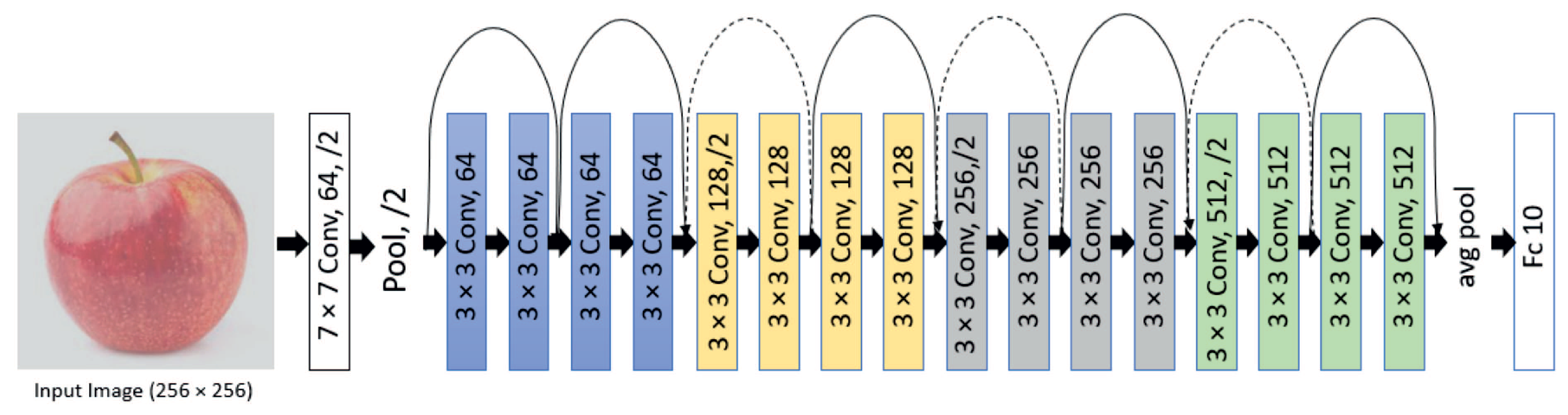
In this contribution, two architectures are used for classification: (1) ResNet18 [20] and (2) MobileNet V2 [21]. In the ResNet18 structure, a Convolutional Neural Network with 18 layers deep is built based on a deep residual learning framework shown in Figure 1.

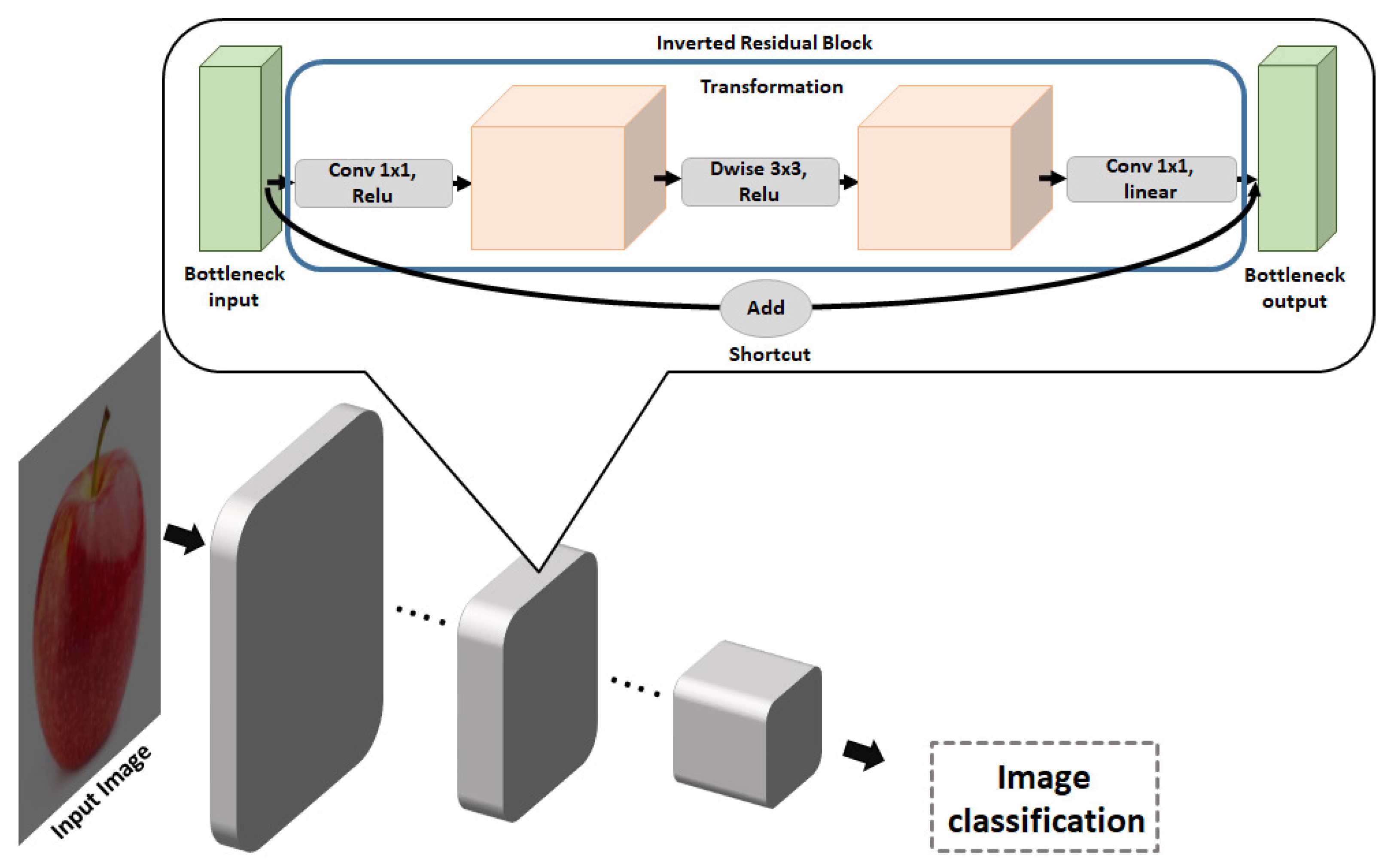
The learning approach eliminates accuracy degradation while the depth of the network increases. In the MobileNet V2 structure, an inverted residual and linear bottleneck layer is proposed to increase the accuracy in mobile and computer vision applications. This structure is an improved version of MobileNet V1 which uses the depth-wise separable convolution to decrease the size of the model and, correspondingly, the complexity of the network. The overall architecture of MobileNet V2 is shown in

Table 1. Overall architecture of MobileNet V2.

Input	Operator	t	c	n	s
${224}^2$× 3	conv2d	-	32	1	2
${112}^2$× 32	bottleneck	1	16	1	1
${112}^2$× 16	bottleneck	6	24	2	2
${56}^2$× 24	bottleneck	6	32	3	2
${28}^2$× 32	bottleneck	6	64	4	2
${14}^2$× 64	bottleneck	6	96	3	1
${14}^2$× 96	bottleneck	6	160	3	2
$7^2$× 160	bottleneck	6	320	1	1
$7^2$× 320	conv2d 1 × 1	-	1280	1	1
$7^2$× 1280	avgpool 7 × 7	-	-	1	-
1 × 1 × 1280	conv2d 1 × 1	-	k	-	-

, and the basic building block shown in Figure 2.

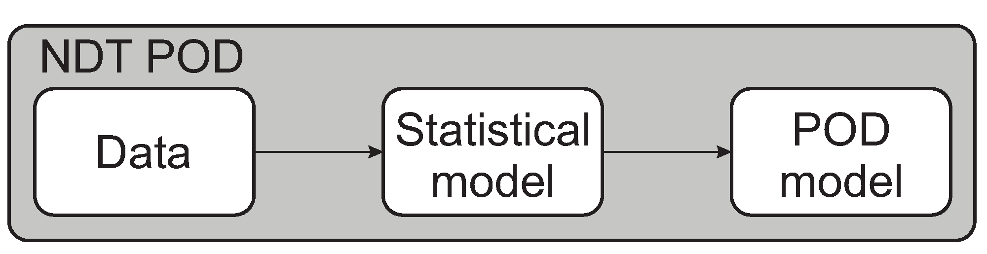
2. POD Assessment of Binary Classifiers

An introduction of the adapted POD [18] and its implementation in classifier evaluation is briefly repeated in this section. Probability of Detection is a certification tool used to assess the reliability of nondestructive testing (NDT) measurement procedures [15,22]. The MIL-HDBK-1823A is the state-of-the-art and contemporary guide for POD studies [23,24]. The evaluation process use the so-called POD curve [15,22]. Data used in producing POD curves are categorized by the main POD controlling parameters. These parameters are either discrete or continuous and can be classified as follows:

• Target response: data which provide quantitative measure of target;
• Hit/miss: produce a binary statement or qualitative information about the existence of a target.

Both approaches are adapted, extended, and implemented as a new performance evaluation metric for vision-based systems.

2.1. Target Response Approach to POD

The target response approach is used when a relationship between a dependent function and an independent variable exists [15]. In the derivation of the POD curve, a predictive modeling technique is required. Regression analysis is one of this statistical regression approaches [15,25,26]. In the derivation of the target response POD curve, a regression analysis of the data gathered has to be realized [25,26]. The regression equation for a line of best fit to a given data set is given by:

$$y=b+mx,$$

(1)

where m is the slope and b the intercept. The Wald confidence bounds are constructed to define a confidence interval that contains 95% of the observed data. Here, the 95% Wald confidence bounds on y is constructed by [27]:

$$y_{(a=0.95)}=y+1.645{\tau }_y,$$

(2)

where 1.645 is the z-score of 0.95 for a one-tailed standard normal distribution, and ${\tau }_y$ is the standard deviation of the regression line. The Delta method is a statistical technique used to transition from a regression line to a POD curve [15]. The confidence bounds are computed using the covariance matrix for the mean and standard deviation POD parameters $\mu$ and $\sigma$, respectively [28]. To estimate the entries, the covariance matrix for parameters and distribution around the regression line needs to be determined. This is performed using Fisher’s information matrix I [28]. The information matrix is derived by computing the maximum likelihood function f of the standardized deviation z of the regression line values. The entries of the information matrix are calculated by the partial differential of the logarithm of the function f using the parameters of $\mathrm{\Theta }(m,b,\tau )$ of the regression line. From

$$z_i=\frac{(y_i-(b+m{x}_i))}{\tau }$$

(3)

and

$$f_i=\prod _{i=1}^n\frac{1}{2\pi }{e}^{-\frac{1}{2}{\left(z_i\right)}^2}$$

(4)

the information matrix I can be computed as:

$$I_{ij}=-E\left(\frac{{\partial }^2}{\partial {\mathrm{\Theta }}_i\partial {\mathrm{\Theta }}_j}log\left(f\right)\right).$$

(5)

The inverse of the information matrix yields $\varphi$ as:

$$\varphi =I^{-1}=\left[\begin{array}{ccc}{\sigma }_b^2& {\sigma }_b{\sigma }_m& {\sigma }_b{\sigma }_{\tau }\\ {\sigma }_m{\sigma }_b& {\sigma }_m^2& {\sigma }_m{\sigma }_{\tau }\\ {\sigma }_{\tau }{\sigma }_b& {\sigma }_{\tau }{\sigma }_m& {\sigma }_{\tau }^2\end{array}\right].$$

(6)

The mean $\mu$ and standard deviation $\sigma$ of the POD curve are calculated by $\mu =\frac{c-b}{m}$, where c is the decision threshold and $\sigma =\frac{\tau }{m}$. The cumulative distribution $\mathrm{\Phi }$ is calculated as:

$$\mathrm{\Phi }(\mu ,\sigma )=\frac{1}{2}\left[\begin{array}{c}1+erf\left(\frac{x-\mu }{\sigma \sqrt{2}}\right)\end{array}\right],$$

(7)

where $erf$ denotes the error function. The POD function is derived as:

$$POD\left(a\right)=\mathrm{\Phi }\left[\begin{array}{c}\frac{a-\mu }{\sigma }\end{array}\right].$$

(8)

Using Equation (8), the POD curve can be set up for varying parameters. In this contribution, the varying parameters (as process parameters) are the contrast and brightness of the image. The intercept and slope are represented by the variables ${\widehat{\beta }}_0$ and ${\widehat{\beta }}_1$, respectively, and are statistically estimated from the observations using the maximum likelihood estimation, as it is better suited for censored regression.

2.2. Hit/Miss Approach to POD

An efficient implementation of the binary data is to posit an underlying mathematical relation between POD and parameter to model the probability distribution [15]. The use of ordinary linear regression is inaccurate due to the fact that the data are not continues but discrete and bounded. Generalized Linear Models (GLM) overcome this challenge by linking the binary response to the explanatory variables through the probability of either outcome, which continuously vary from 0 to 1 [15,27]. The GLM attains this through:

1.

A random component specifying the conditional distribution of the response variables, $Y_i$ (for the i-th of n independently sample observations);

2.

A linear predictor that is a function of regressors;

3.

A smooth and invertible linearizing link function $g\left(y\right)$, which transforms the expectation of the response variables $P_i\equiv E\left(Y_i\right)$ to the linear predictor.

The transformed probability can then be modeled as an ordinary polynomial function, linear in the explanatory variables. The commonly used GLM in POD are the Log, Logit, Probit, Loglog, and Weibull link functions. Depending on the data distribution, a model may be more appropriate compared to another. One criterion used is to select the GLM with the least deviance.

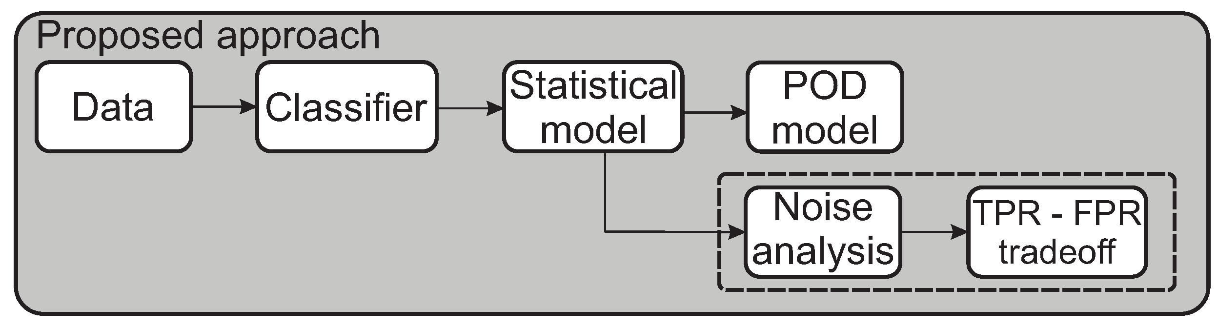
The target response and the Hit/Miss approaches are adapted as a new performance evaluation for vision-based classifiers. The classical POD approach utilized in the field of NDT is shown in Figure 3.

The POD approach is adapted, modified, and extended to the field of vision-based systems as shown in Figure 4. This article adapts the method; however, unlike classical POD applications, for the first time, the method is applied to process-parameter-affected vision-systems. Here, raw sensor/probe data are not used, but a prefilter in the form of a classifier is used. The classifier is evaluated based on the processed data. Additionally, a noise analysis procedure is introduced, fully illustrating the visualization and trade-off between the decision thresholds, image parameters, detection probabilities, and false positive rates.

3. Classification Results

In this contribution, a custom dataset proposed by [29] is used for the experiments. The dataset contains 43,956 images, of which 38,456 are used for training and 5500 for validation. The dataset contains 11 classes (apple, atm-card, cat, banana, bangle, battery, bottle, broom, bulb, calendar, camera). Considering 11 different classes, the ground-truth is a one-hot vector of size 11. At each parameter intensity, the assignment is 1 (Hit) for correctly classified image and 0 (Miss) for a wrong classification. Both ResNet and MobileNet V2 are trained for 10 epochs on the customized dataset using the transfer learning approach [30]. The pre-trained version of ResNet and MobileNet V2 on the ImageNet dataset [31] is used in the experiment. Achieving high classification accuracy on the customized dataset is faster using pre-trained models trained on similar datasets. The classification results are detailed in

Table 2. Classification results.

Model	Training Accuracy	Validation Accuracy
ResNet18	0.995	0.9878
MobileNet V2	0.9621	0.976

.

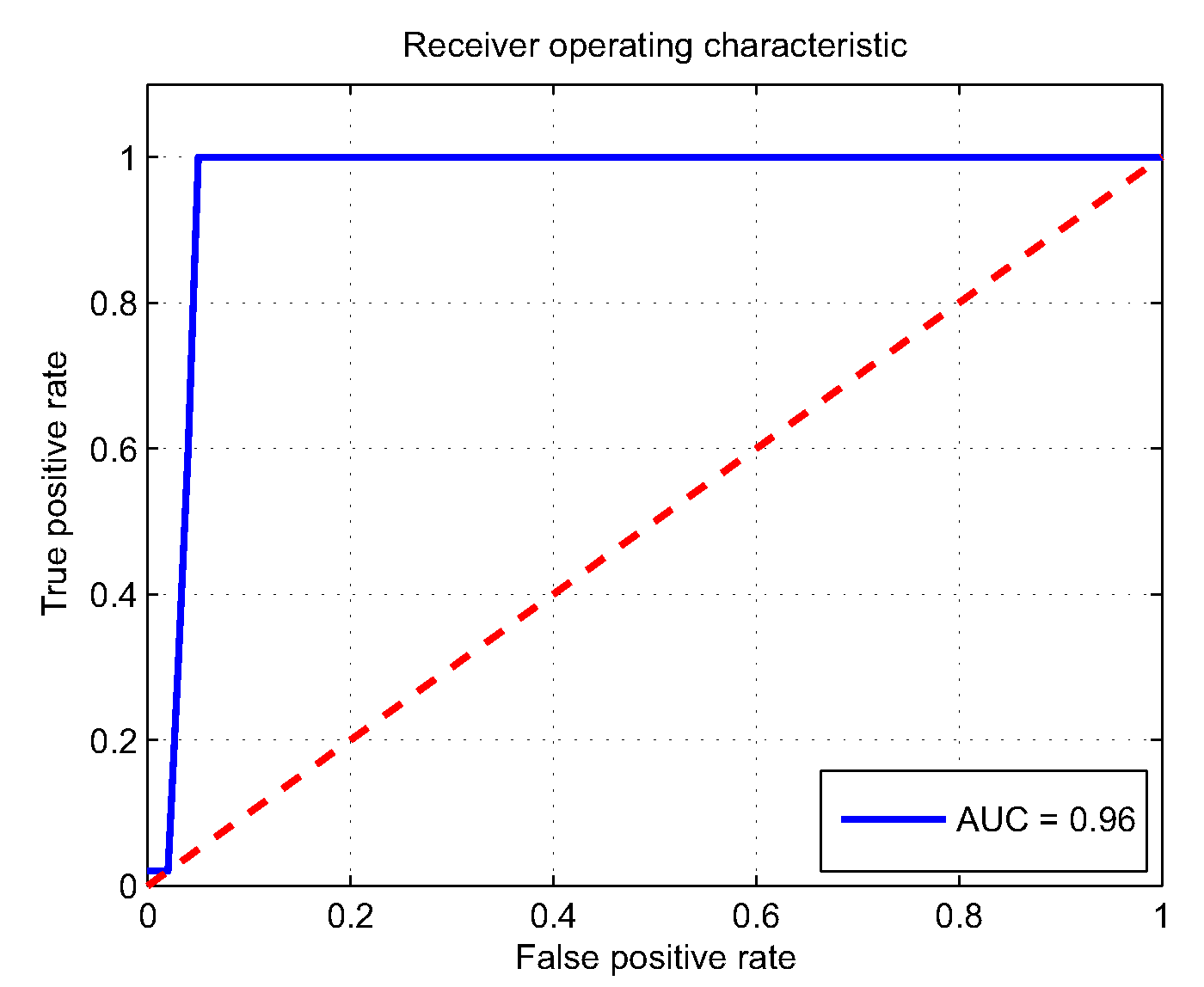
To elaborate the benefits of proposed method the ROC curve and the accuracy curve are considered (Figure 5 and Figure 6). The generated ROC curve is shown in Figure 6. The graph shows the true positive rate against the false positive rate, while the decision threshold is varied. The ROC curve indicates relative compromises between true positives (benefits) and false positives (costs) and is not able to show the effects from the process parameter. For contemporary applications, the influence of the process parameter is critical, so the detection probability should be related to severity. In this instance, the process parameter is a surrogate for severity. Currently, there are no alternatives to incorporating the process parameter, hence the need for the POD approach.

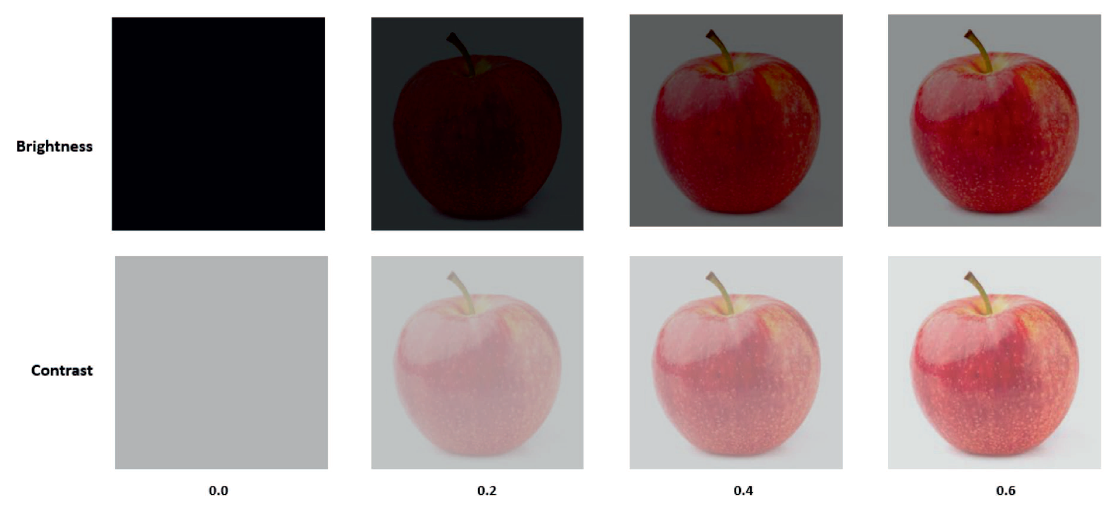
4. New Evaluation of Object Classification by the Target Response Approach

The classifiers are used to classify/identify apples from an image. Two image parameters are considered as the varying parameters: contrast and brightness (Figure 7).

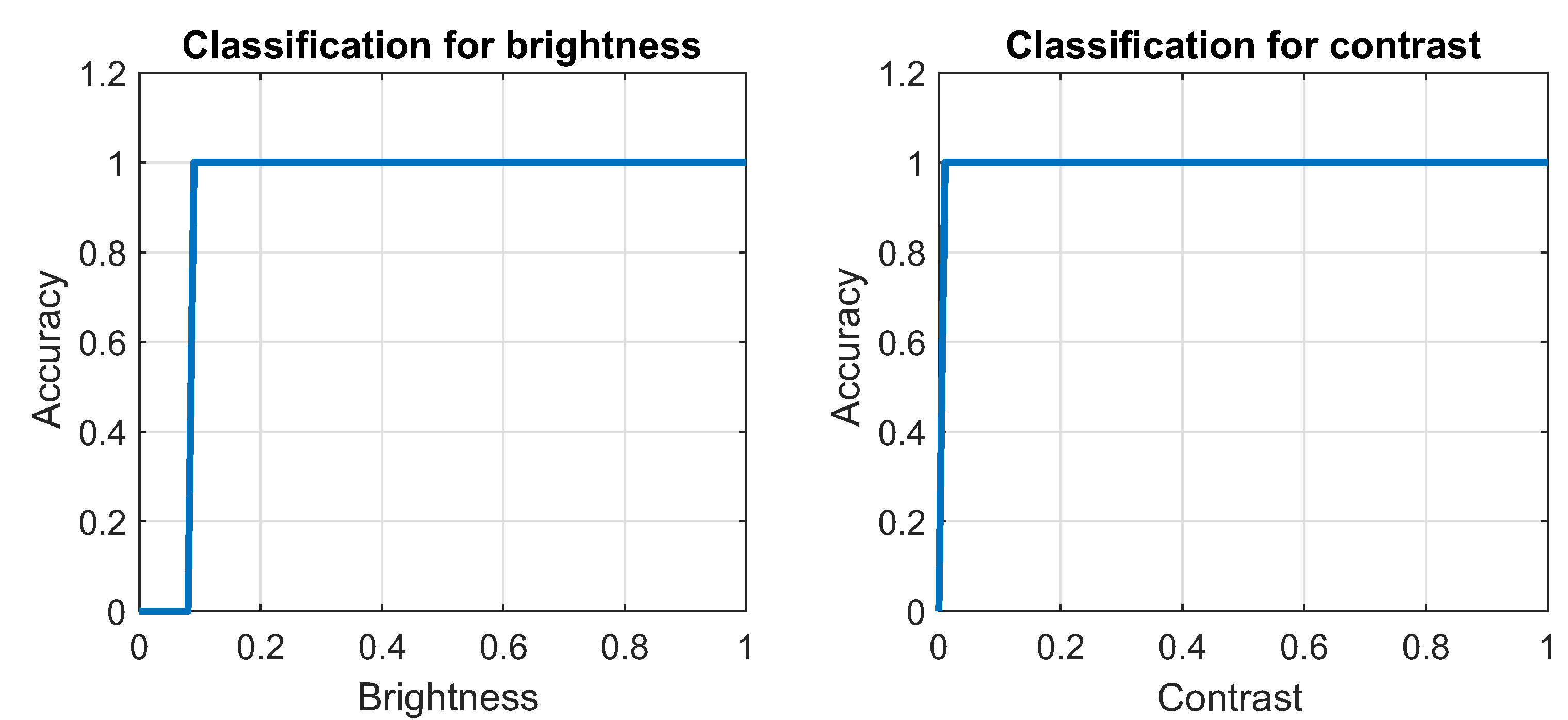
The target response approach is adapted and implemented as a new performance assessment for classification approaches. In this section, the MobileNet V2 classifier is implemented. The contrast is varied from 0 (min) to 1 (max). Beyond a contrast value of 0.2, the algorithm is able to detect the image with a probability of 99.94% (see

Table 3. Probability of Detection considering different image contrasts.

Contrast	Probability
0	0.31452537
0.1	0.72617805
0.2	0.9944179
0.3	0.9994198
0.4	0.99984
0.5	0.9999324
0.6	0.99995387
0.7	0.99997306
0.8	0.99997616
0.9	0.9999759
1	0.9999771

).

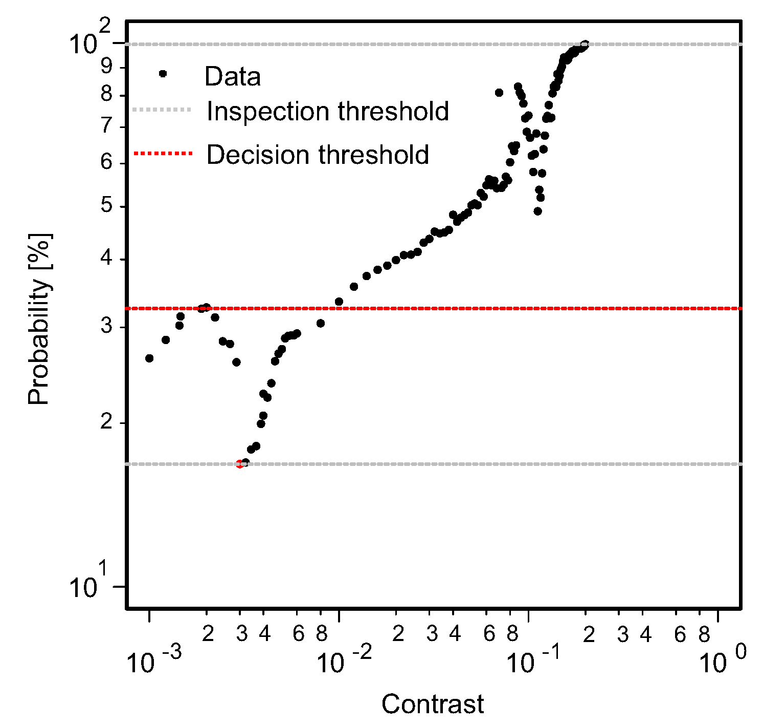
Therefore, the analysis is made for the range of 0 to 0.2. Beyond 0.2, the algorithm reaches a saturation threshold and has no effect on POD characterization. We examine 100 contrast values between 0 and 0.2 and the corresponding probability values.

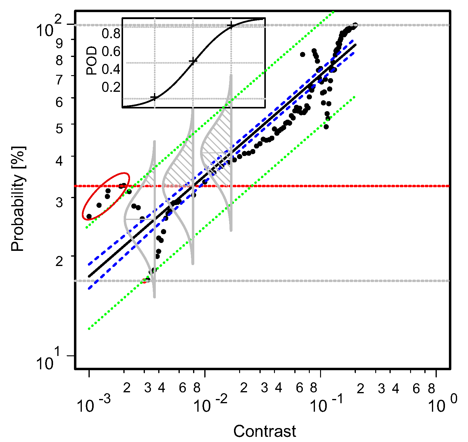
A graph of the data is illustrated in Figure 8. The inspection threshold (least detectable target), saturation threshold (maximum detectable target), and decision threshold (threshold below which the observed data are characterized as noise) are constructed.

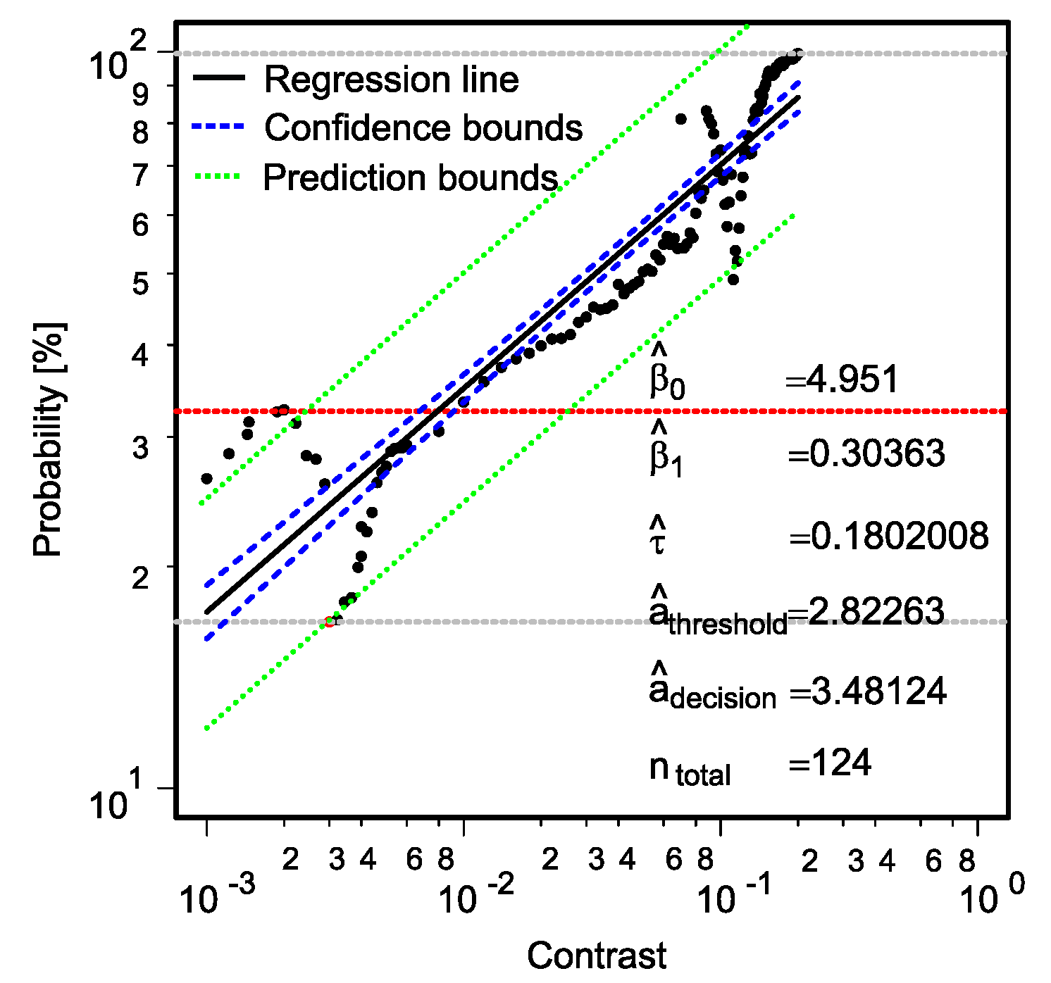
To establish a POD characterization illustrating the effect of the process parameter, contrast values are examined. A regression analysis is carried out for the dataset. The 95% confidence bounds and the prediction bounds are also constructed (see Figure 9).

The confidence bounds are constructed for certification purposes while the prediction bounds serve as boundaries so that for every new 100 observations, 95 should fall within. The cumulative density functions (CDF) for the data distribution are also constructed. The POD curve is generated using area of the cumulative density function above the decision threshold (Figure 10).

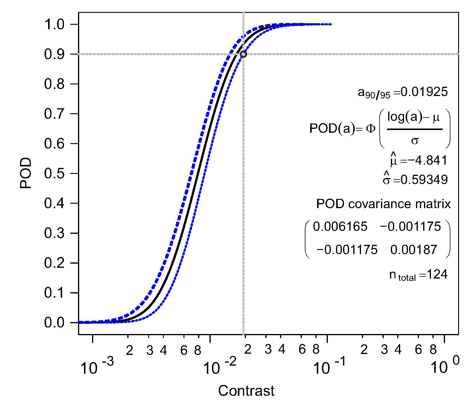
The confidence bounds about the regression line are used in constructing the 95% bounds around the POD curve.

The 90/95 certification criteria representing a 90% probability of detecting the image with a reliability of 95% is utilized in this contribution. The 90/95 (o in Figure 11) value for this concrete example is 0.02167. This implies that, in varying the contrast values at 0.02167, the algorithm is able to detect the image with 90% probability at 95% reliability. This developed approach provides a new evaluation and performance assessment for classifiers incorporating the effect of image property on the classification results. From Figure 10, it is evident that the probability density for the classifier changes with the parameter (here: contrast). This visualization is not possible using the ROC or PR curve. However, the POD curve does not give any indication of the false call for any selected decision threshold. To compute the false call, noise will be analyzed in the next section.

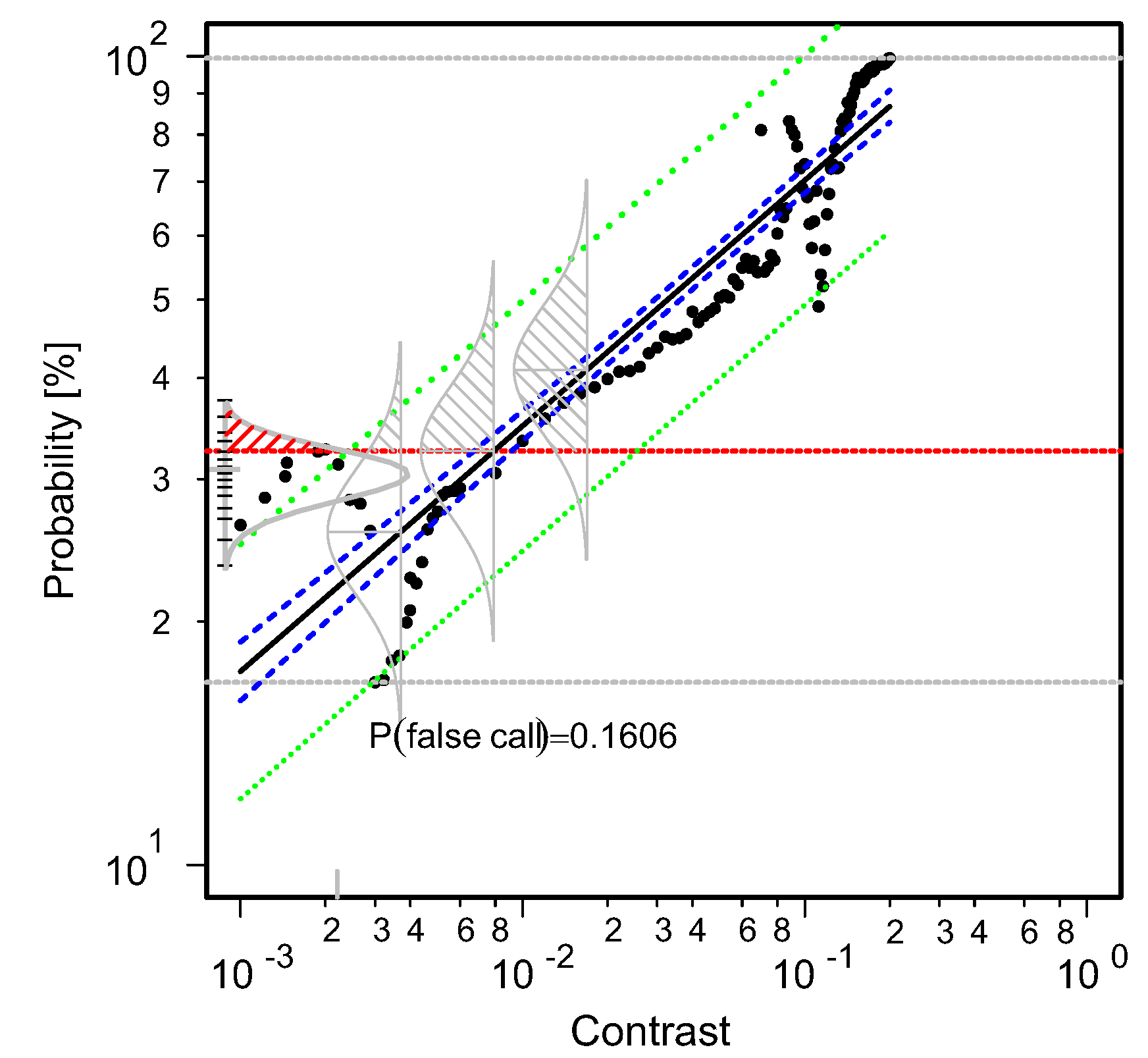
5. False Call Analysis

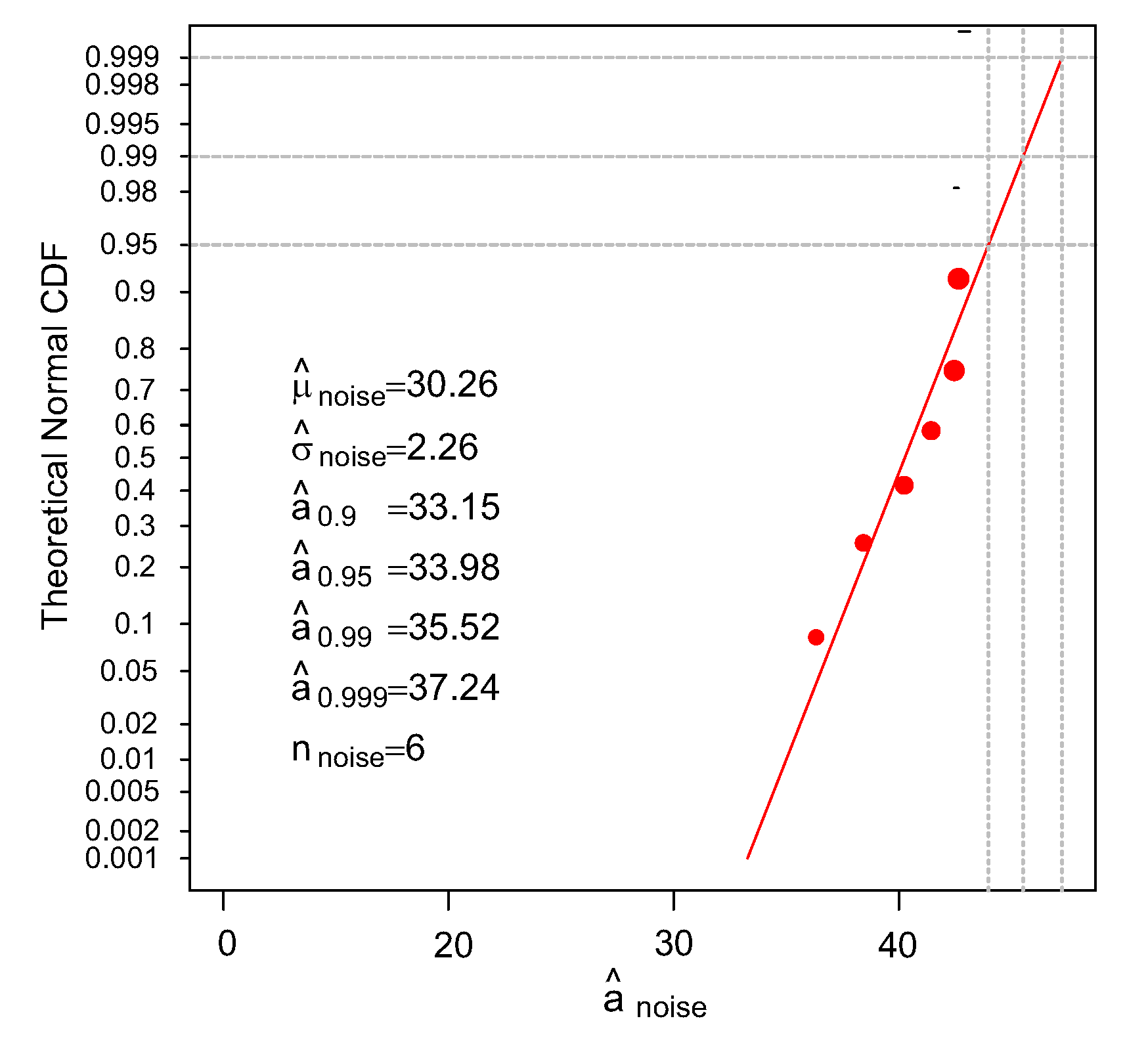
The observed data aggregate the characteristics of the targets signature corrupted by aberrant signals generally referred to as noise. Classical POD methods usually measure noise as part of planned experimental measurements, however, that is absent in the current work. Noise, therefore, will be inferred from the observed data. Noise in this context refers to observed signals with no useful target characterization information. Therefore, observed data outside the prediction bounds will be interpreted as noise because the corresponding POD is zero. Still using data from Figure 10, the noisy data refer to the red circled data in Figure 10. The extracted noise and the corresponding noise parameters are shown in Figure 12.

The false call or probability of false positive (PFP) can be calculated as the noise distribution above the selected threshold. The PFP is computed as:

$$PFP=P(y_{noise}>y_{th})$$

(9)

A statistical ${\chi }^2$ (Chi-squared) hypothesis test is undertaken to identify the nature of noise distribution. Various distributions are tested. The Gaussian distribution emerges as the most plausible. An analysis is carried out on the noisy data, and the mean ${\mu }_{noise}$ and standard deviation ${\sigma }_{noise}$ are calculated.

For a Gaussian distribution, the probability of false call is computed as:

$$PFP={\int }_{y_{th}}^{\infty }\frac{1}{\sqrt{2\pi }{\widehat{\sigma }}_{noise}}{e}^{-\frac{{(y-{\widehat{\mu }}_{noise})}^2}{2{\widehat{\sigma }}_{noise}^2}}dy.$$

(10)

The distribution with regards to PFP is illustrated in Figure 13 (shaded red area relative to the selected decision threshold).

From Figure 13, it becomes evident that for a selected decision threshold (DT), a corresponding unique FAR value exists; however, the detection probability varies relative to a parameter (here: contrast). This implies that the premise for the construction of the ROC/PR curve for applications requiring the incorporation of process parameter is deficient. This is because for a selected cut-off point there is not one FAR to one DR value but one FAR to many DR values. This consideration was not factored initially because the size of opposition objects/planes during WWII was irrelevant, but modern applications are concerned with how the characteristics of target change the probability of detecting it. Relative to this specific example, for a selected decision threshold of 3.5, the PFP value is 0.1606. To evaluate the PFP corresponding to all thresholds and the associated POD, a trade-off analysis is presented next.

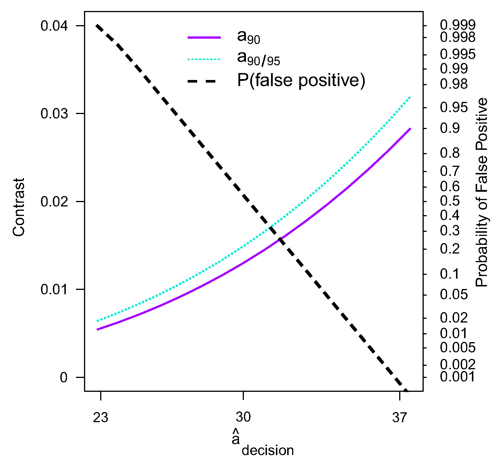
Trade-Off between PFP and POD

From the developed approach, it is possible to analyze the trade-off between PFP and POD. To introduce the novel approach, a single probability point is analyzed. Here, the 90% probability is used and drawn to intercept POD and confidence curves (see Figure 11). At the point of intersection, the POD, PFP, decision threshold, and the process parameter (here: contrast values) are known. These values are considered for every point on the drawn 90% probability line. A graph depicting the relationship between the POD, PFP, DT, and contrast is shown in Figure 14.

The Figure 14 makes it possible to visualize the relationship between the POD, PFP, DT, and process parameter, which is not possible using the ROC curve. To analyze other probabilities required for evaluating the specific points, as is performed for the 90% probability, the introduced method presents a novel and significant approach to concurrently examine all properties affecting the classification results.

6. Comparison of Different Neural Network Models by the Hit/Miss Approach

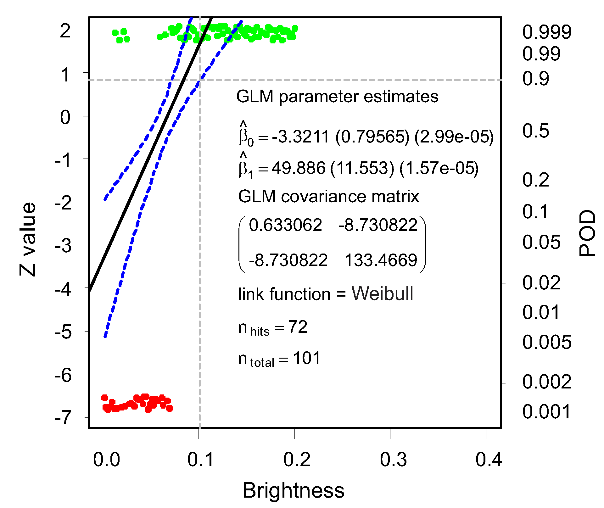
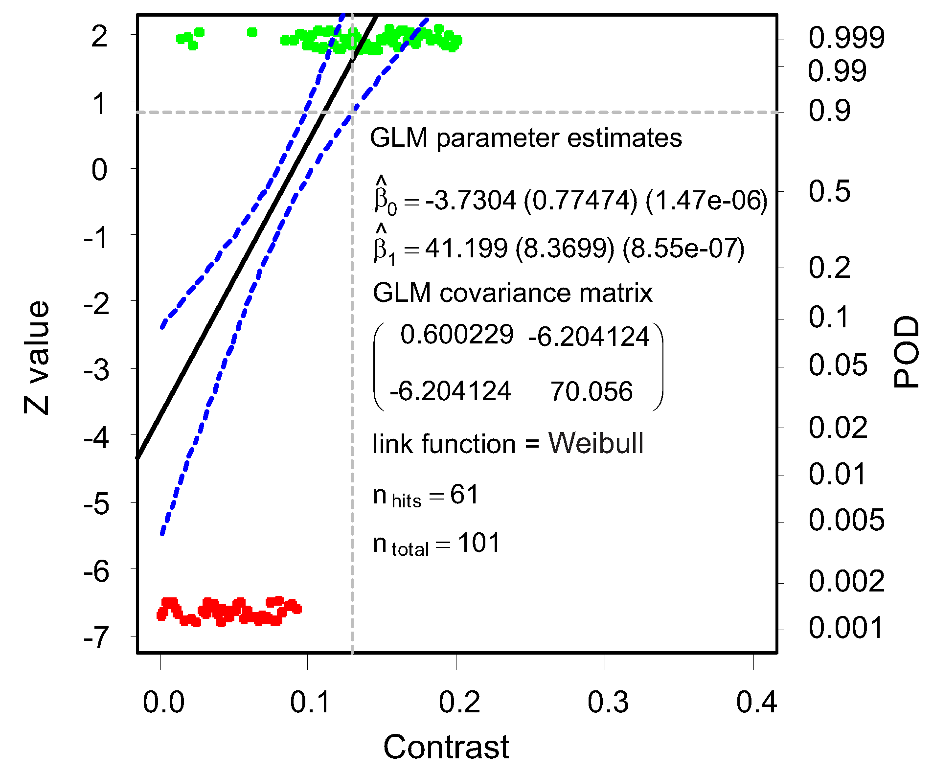
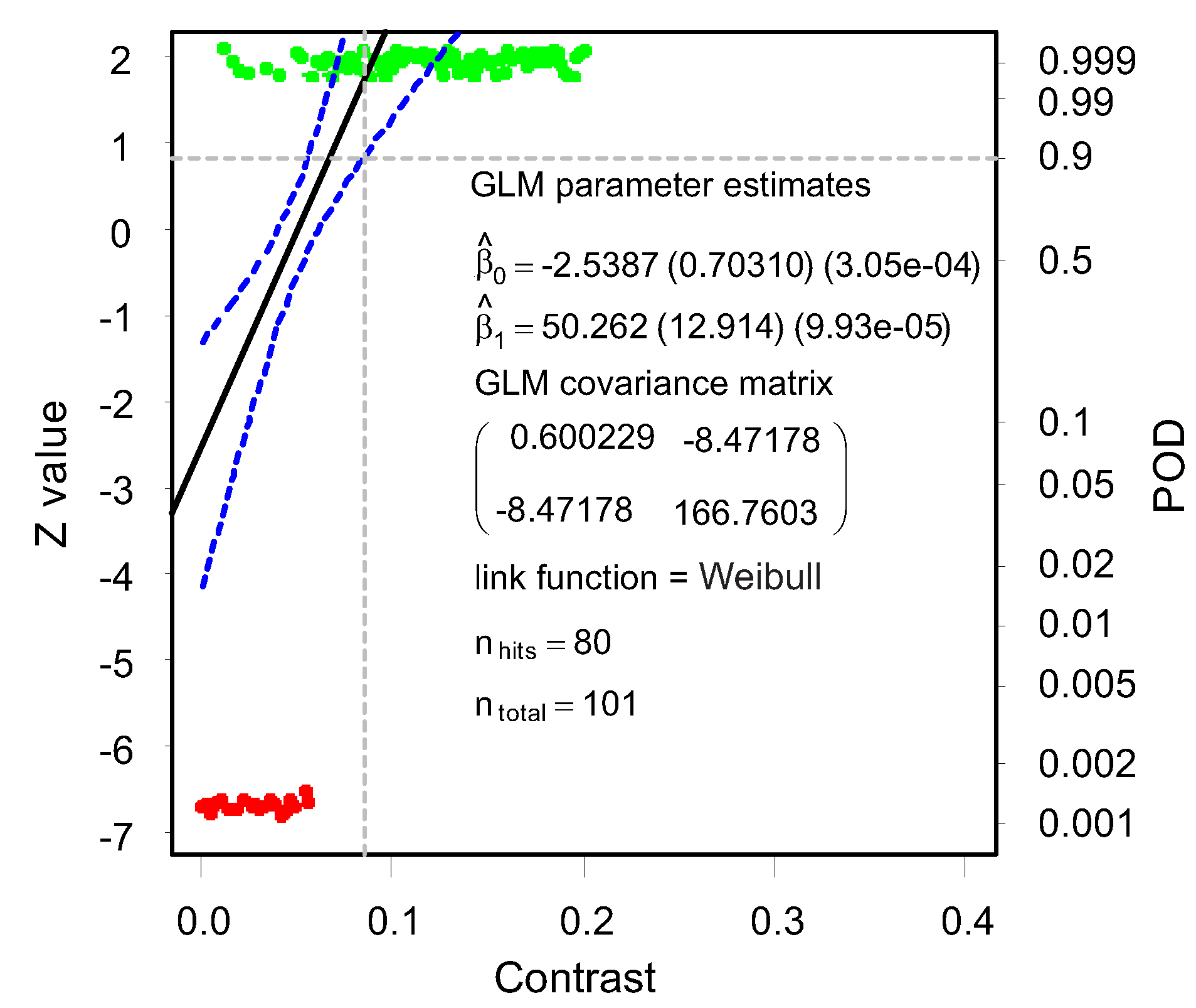
In this section, the Hit/Miss approach is used to evaluate the performance of two Neural Network algorithms, namely, MobileNet V2 and ResNet. Each model is implemented on two varying parameters, namely, brightness and contrast. Here, the classes as opposed to the probabilities are used. The classes are binary in nature, and hence the Hit/Miss approach will be used. At each parameter intensity, if the algorithm classifies the image correctly, a value of 1 (Hit) for a correct class and 0 (Miss) for a wrong class is assigned. Like the former approach, the analysis is made for parameter changes from 0–0.2 at a step size of 0.002.

For binary data, the log-odds distribution is found to be of good fit [22] by linking the binary response to the explanatory variables through the probability of either outcome, which does vary continuously from 0 to 1. The POD function for binary data can be expressed as:

$$POD=\frac{e^{\frac{\pi }{\sqrt{3}}\left(\frac{lna-\mu }{\sigma }\right)}}{1+e^{\frac{\pi }{\sqrt{3}}\left(\frac{lna-\mu }{\sigma }\right)}}.$$

(11)

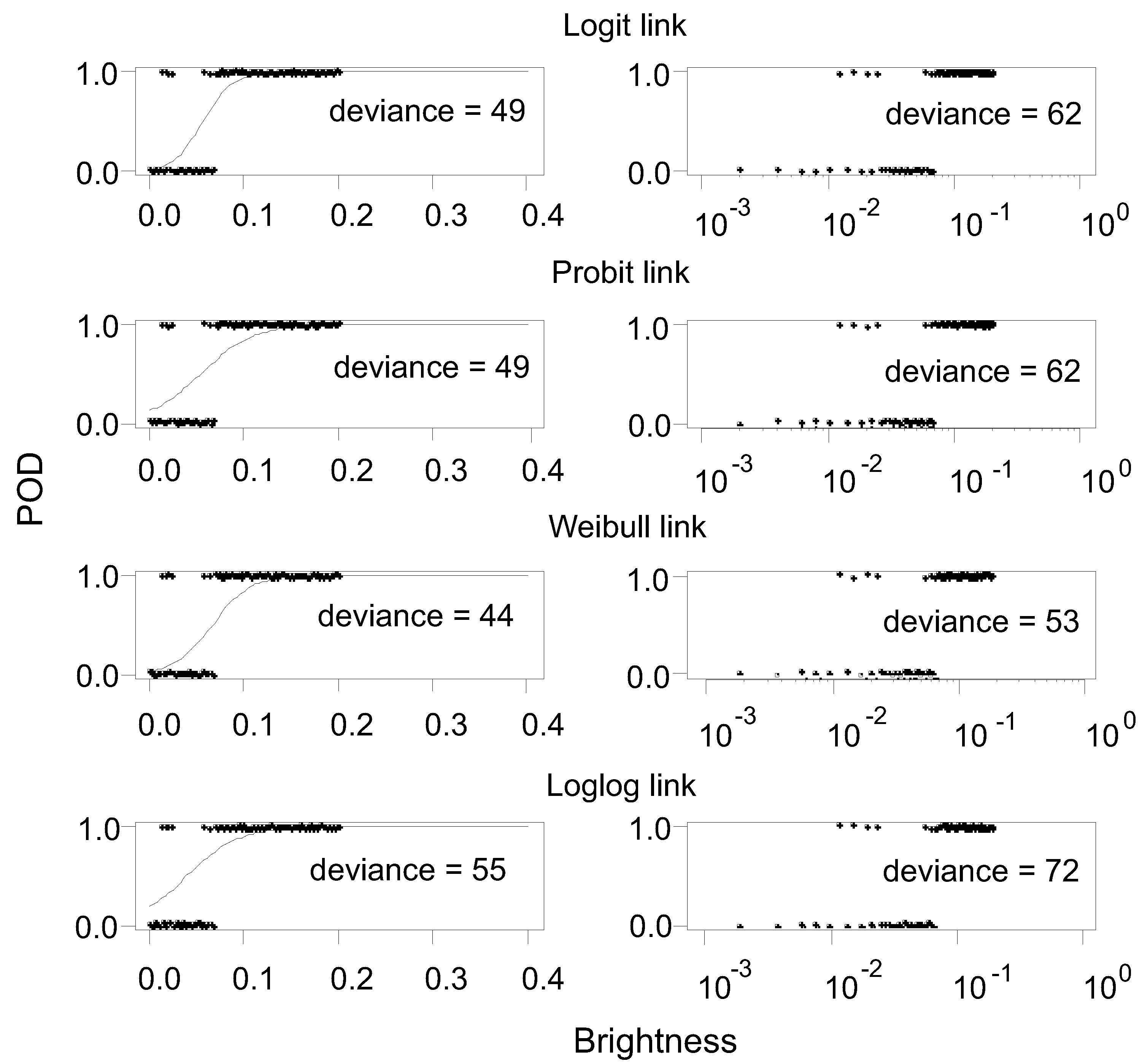
To accurately implement the Hit/Miss approach, the appropriate link function to be used needs to be determined. For illustrative purpose, the classification results of MobileNet V2 considering brightness values are used (Figure 15).

Eight of different link functions are constructed to select best fitting model as illustrated in Figure 15. The data distribution of the logarithmic model does not support the construction of a valid POD curve estimate, and hence, the Cartesian models will be more suitable for this example. A statistical hypothesis testing procedure is undertaken to ascertain the best-fitting link function model. To model the relationship of GLM, deviance is a measure of goodness of fit: The smaller the deviance, the better the fit. It is attained using a generalization of the sum of squares of residuals in ordinary least squares to cases where model-fitting is achieved by maximum likelihood. The Cartesian Weibull link function is selected for this specific analysis because it has the least data deviance in comparison to the other link functions. The procedure is repeated for MobileNet V2 contrast parameter, as well ResNet brightness and contrast parameters. The hypothetical testing procedure show that Cartesian Weibull is the best link function for all. The Weibull is implemented to map $-\infty <x<\infty$ to $0<y<1$. The Weibull function is expressed as

$$f\left(X\right)=g\left(y\right)=log(-log(1-p\left)\right),$$

where $f\left(X\right)$ is an algebraic function with linearized parameters and p the probability. The probability of detection as a function of brightness B for the Weibull model is

$$POD\left(B\right)=1-exp(-exp(f\left(X\right)\left)\right).$$

Using Weibull, surface contours are constructed to ascertain the most plausible GLM (Figure 16, Figure 17, Figure 18 and Figure 19).

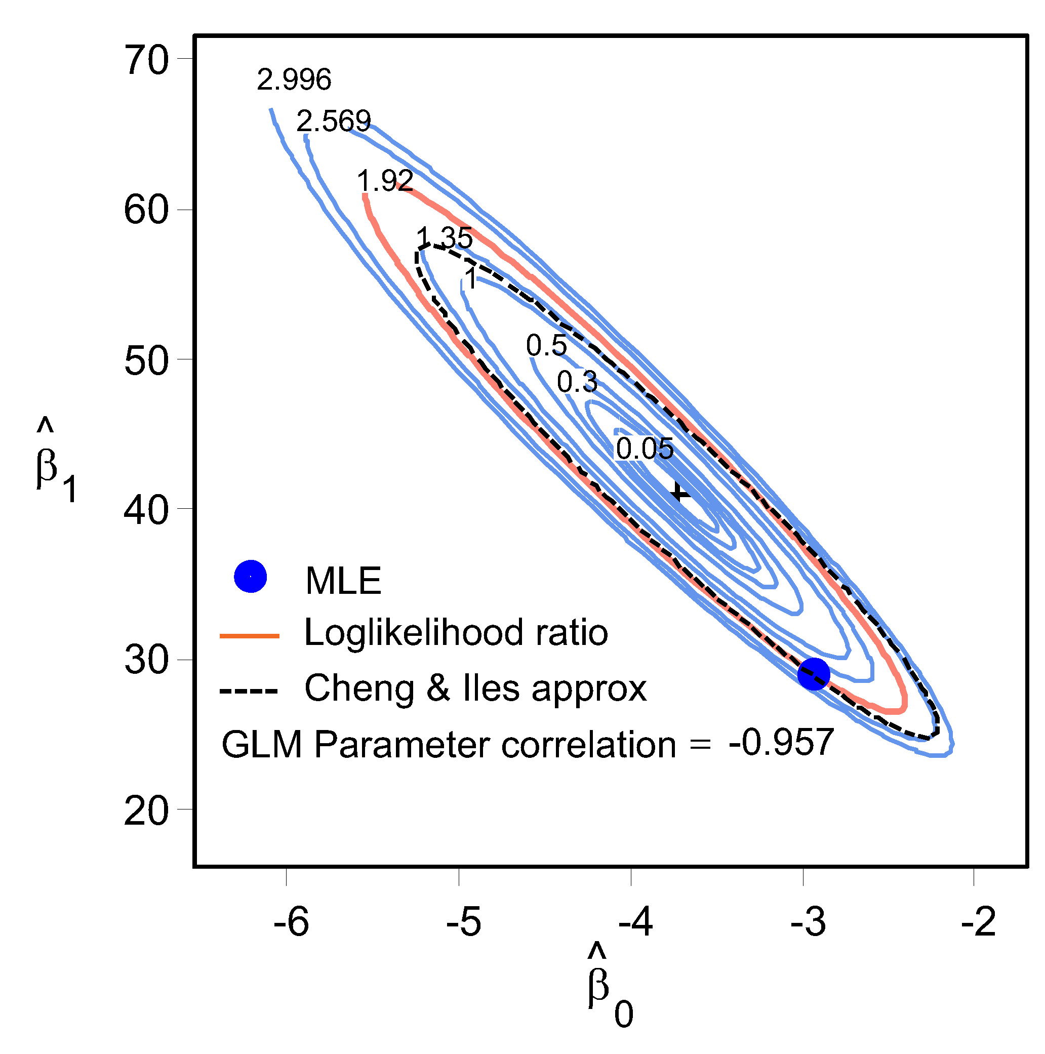
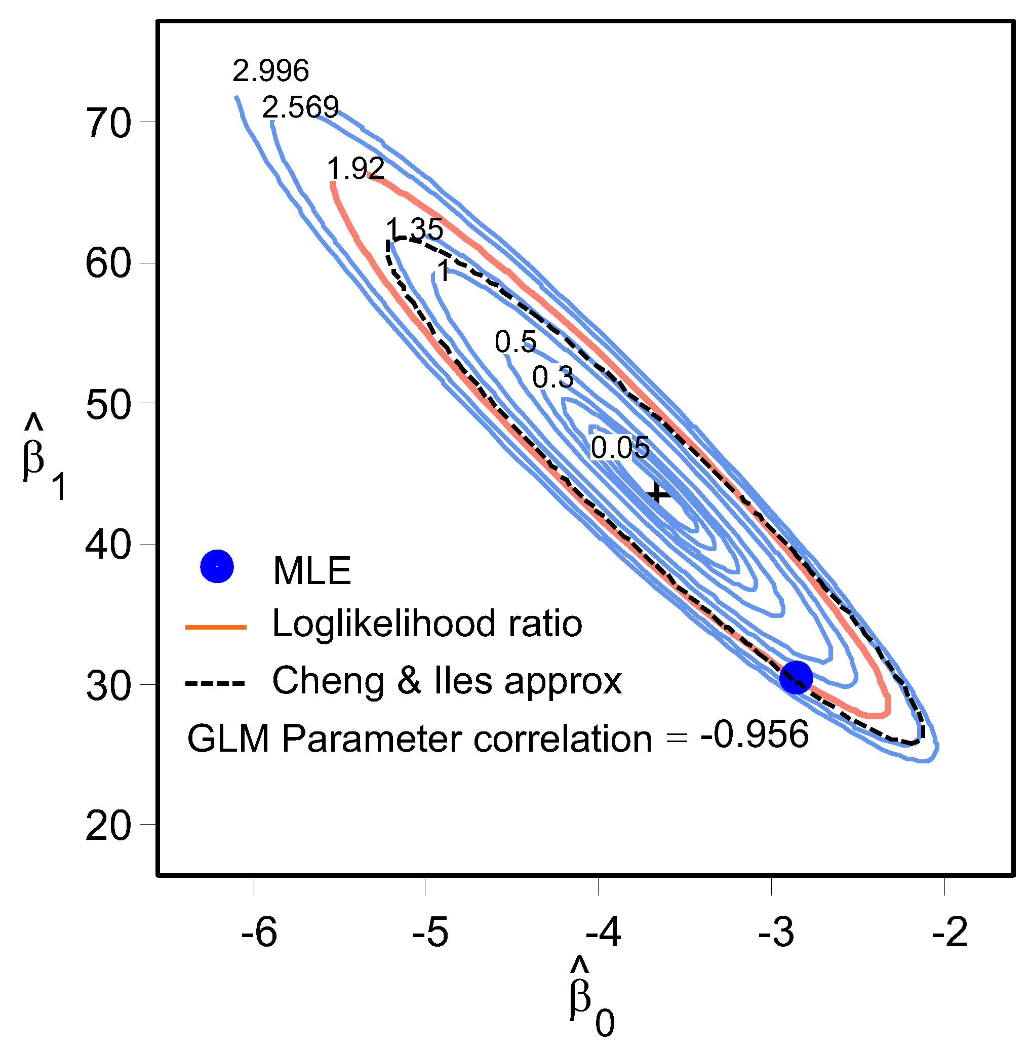
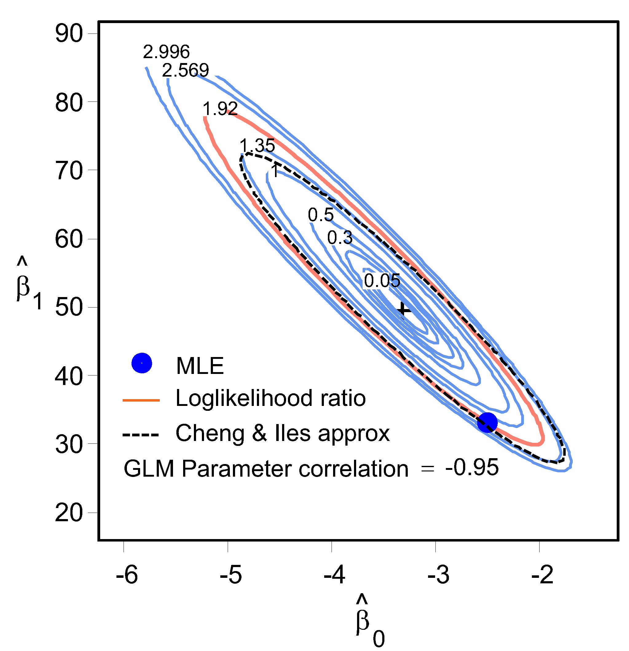
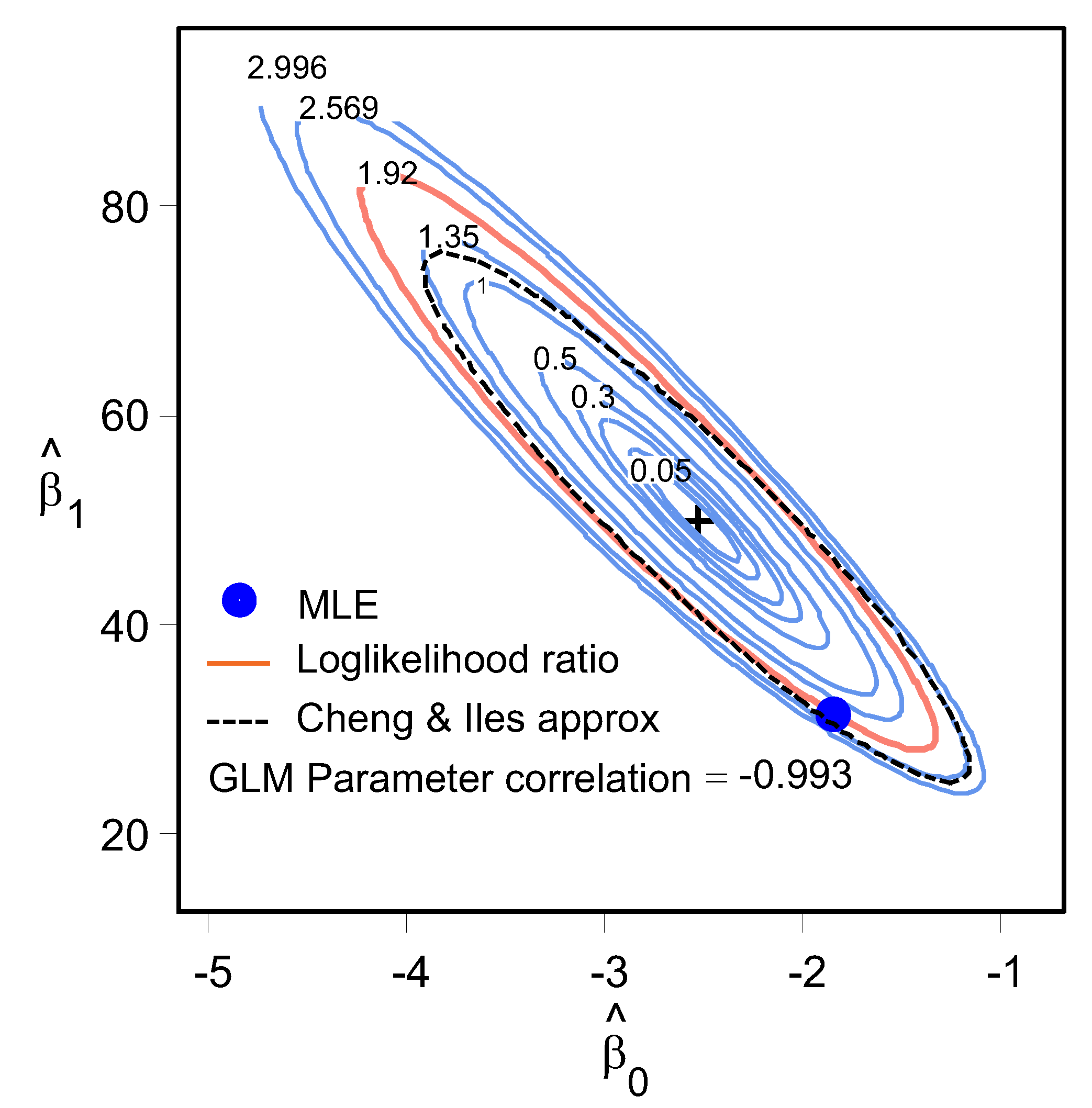
The likelihood ratio test is used to assess the goodness of two competing statistical models based on the ratio of their likelihoods. The log likelihood ratio contour encloses all ${\beta }_0,{\beta }_1$ pairs that are plausibly supported by the data. The confidence bounds are constructed on the surface contours using a method developed by the Cheng & Iles approximation [28].

Using the maximum likelihood estimation (MLE) method, the GLM values for the intercept and gradient are generated for both classifiers. With these values, a GLM model and confidence bounds fitting the data are constructed (Figure 20, Figure 21, Figure 22 and Figure 23).

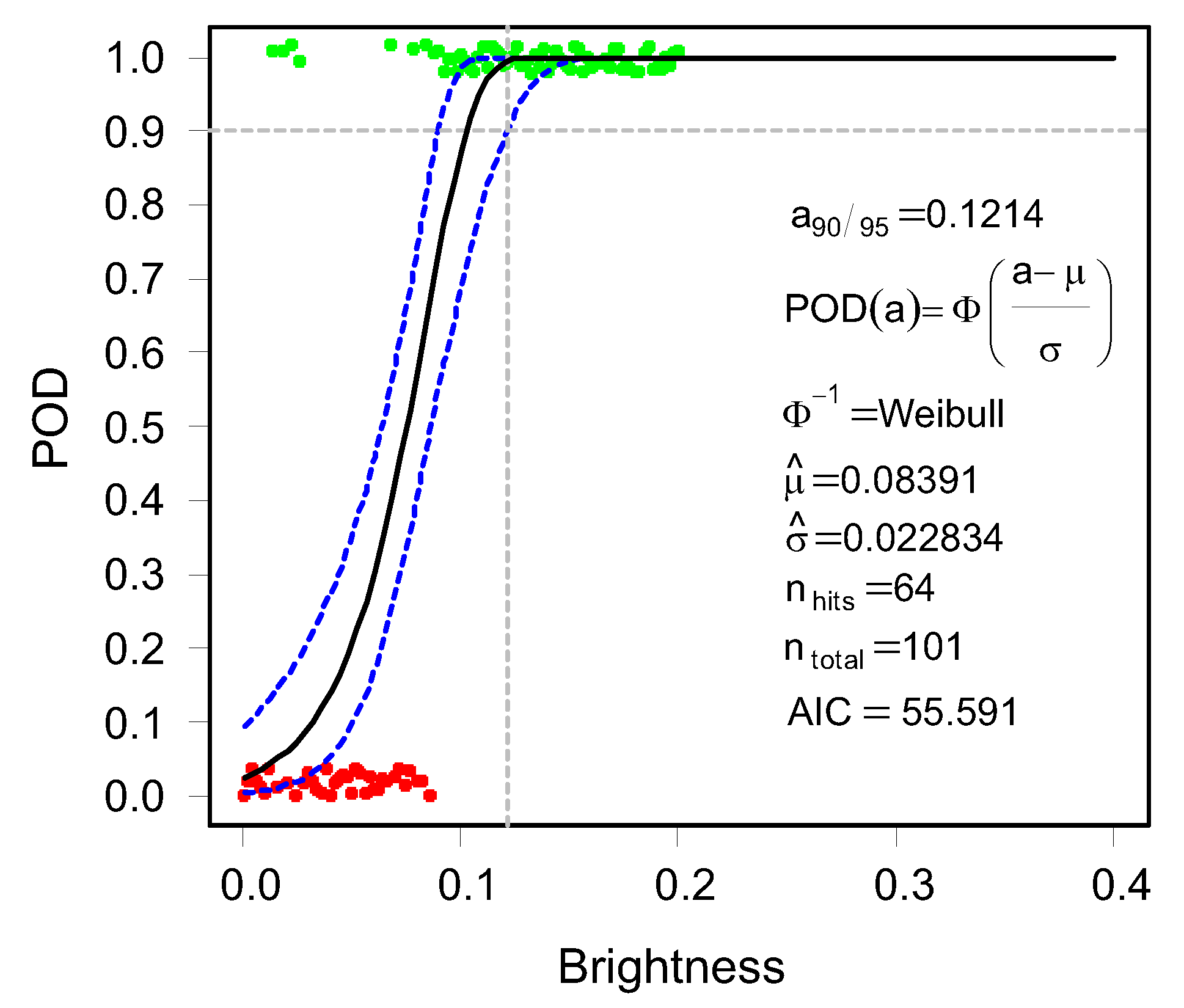
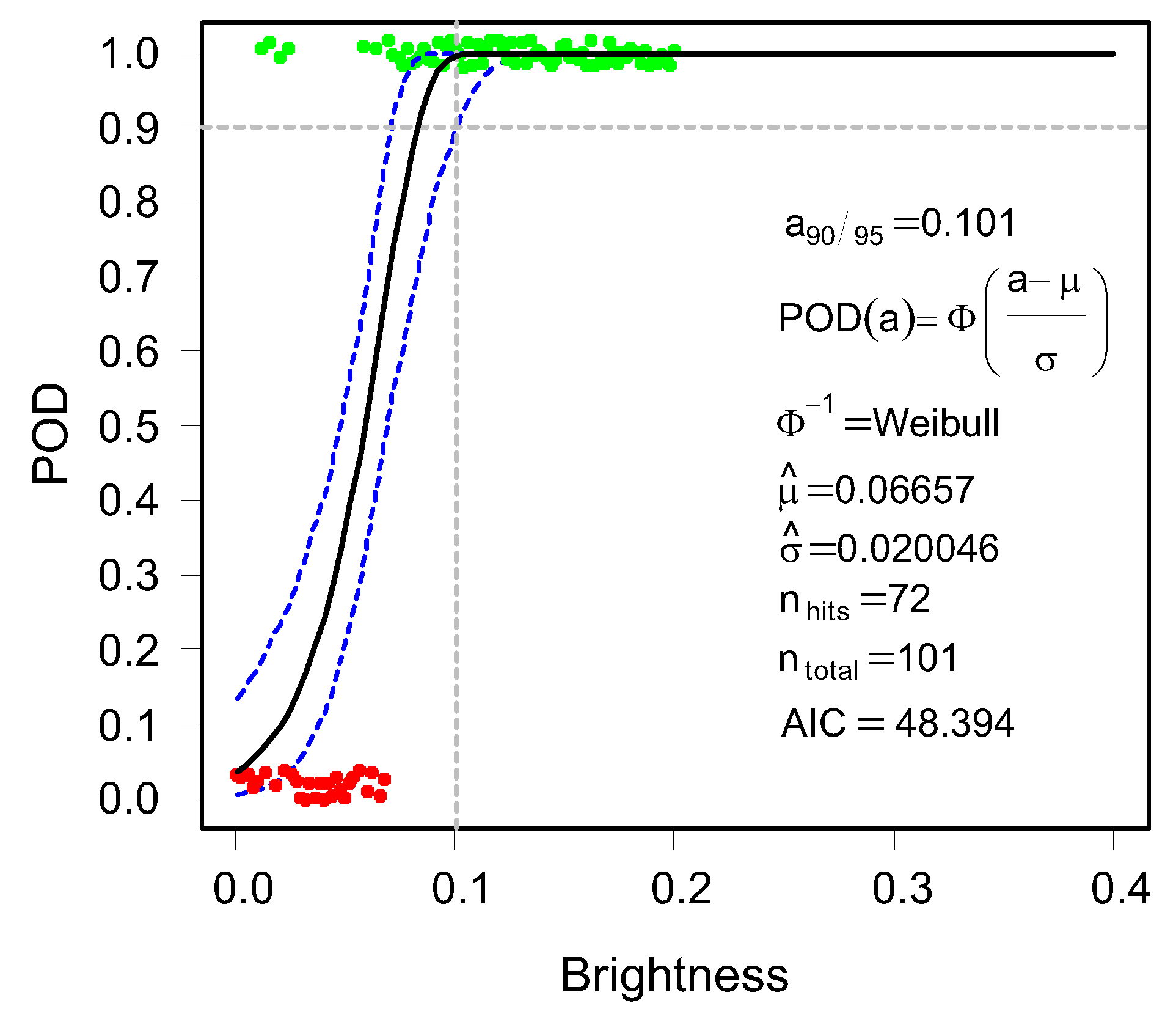
From the fitted GLM model, the POD curve is generated using the parameter estimates (Figure 24, Figure 25, Figure 26 and Figure 27). The 90/95 criteria is also successfully implemented on the results.

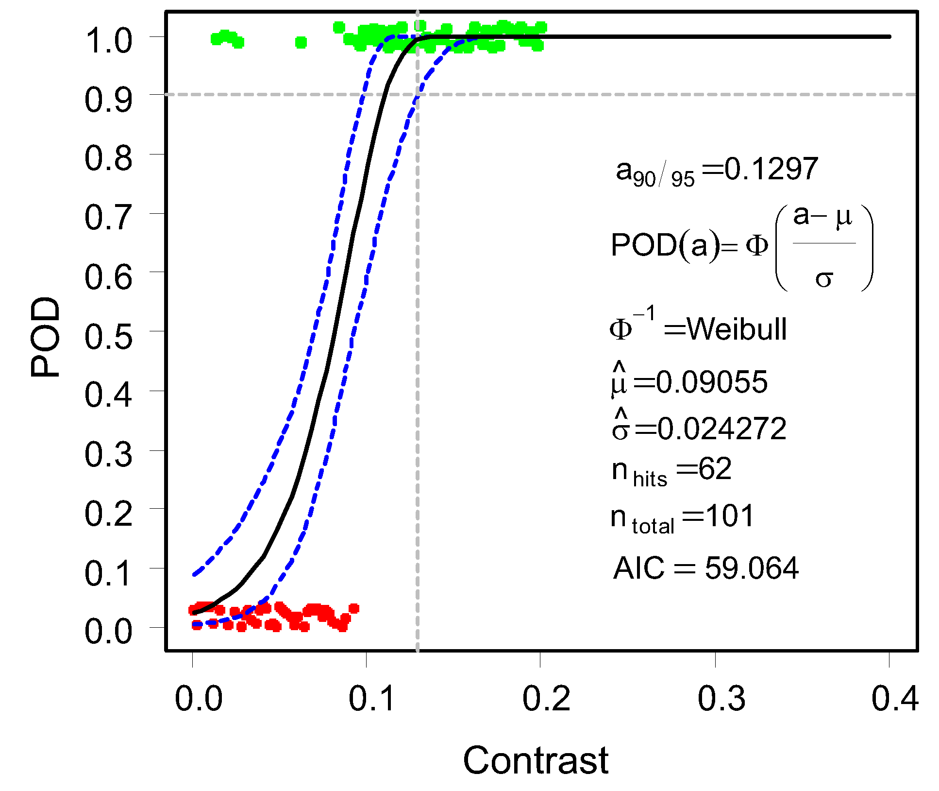
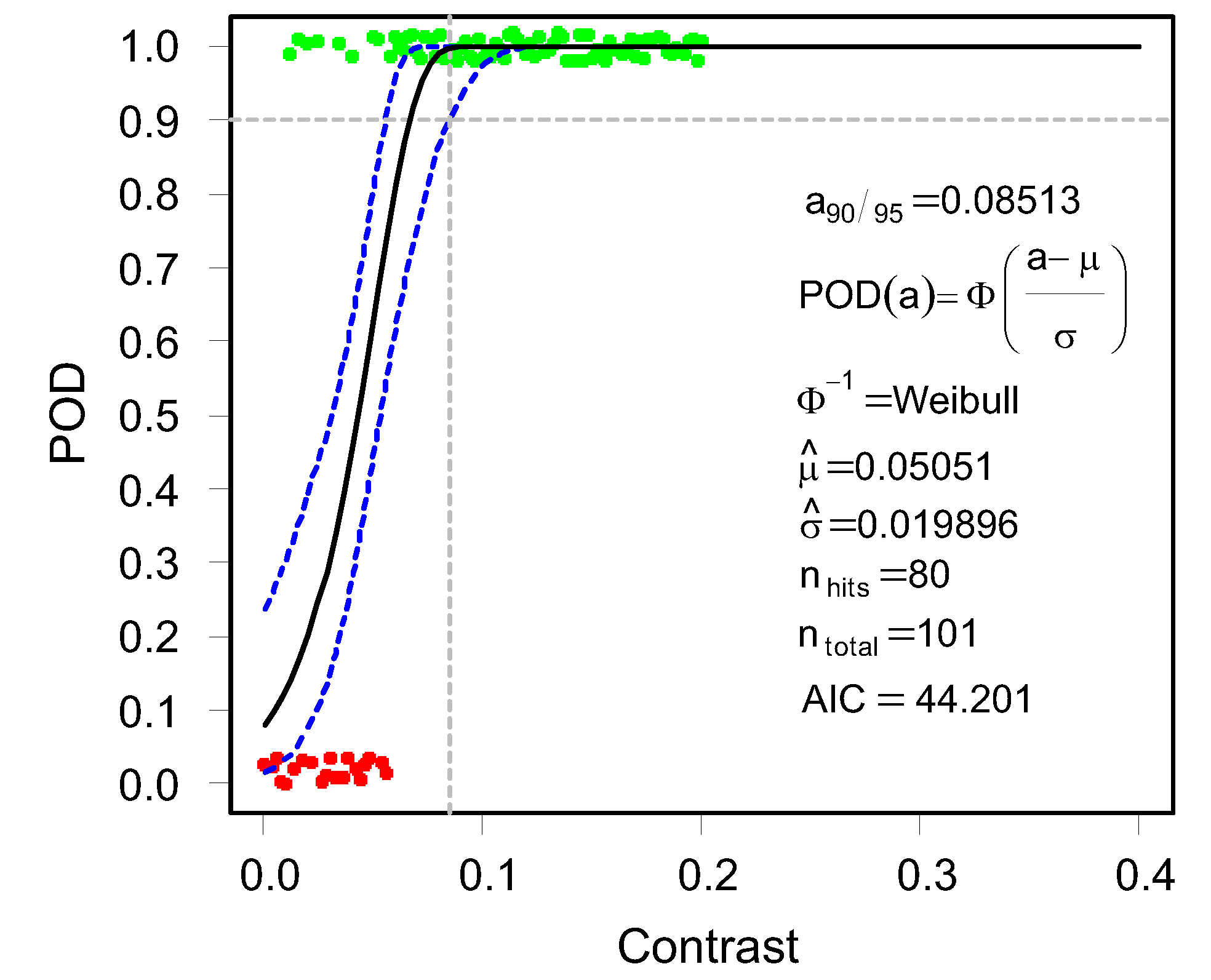
The 90/95 reliability value for MobileNet V2 is 0.101. This implies at the exact brightness intensity value of 0.101, the MobileNet V2 algorithm is able to detect the image with 90% probability at a 95% reliability level. The procedure is repeated for MobileNet V2 contrast, ResNet brightness, and ResNet contrast parameters. A comparison of the 90/95 POD values for the two classifiers and image parameters are detailed in

Table 4. The 90/95 POD values.

Classifier	Brightness	Contrast
MobileNet V2	0.1010	0.1297
ResNet	0.1214	0.0851

.

The smallest 90/95 POD values define the best results because the classification algorithm is able to detect the image at 90/95 reliability with the least contrast/brightness changes. The results (see Table 4) indicate Mobile2Net V2 is more sensitive using brightness values; 0.1010 compared to 0.1214 for ResNet, while ResNet is more sensitive using contrast values; 0.0851 compared to 0.1297 for MobileNet V2.

This POD approach introduces a new performance evaluation for vision-based classification models incorporating and assessing directly the effects of image parameters.

The introduced approach makes it possible to check the number of target hits and missed directly from the POD curve. For the classification results, there are no misses beyond 90/95 ceiling. The hits beyond 90/95 for the classifiers and different parameters are detailed in

Table 5. Hits beyond 90/95 POD.

Classifier	Brightness	Contrast
MobileNet V2	50	36
ResNet	40	58

.

Using this specific example it can be shown that the evaluation and prediction system is reliable for all classification results because no misses are observed beyond the POD ceiling (90/95 threshold). For brightness parameters, MobileNet V2 has 50 hits beyond the 90/95 threshold compared to 40 for ResNet. For the contrast parameter, MobileNet V2 has 36 hits beyond the 90/95 threshold compared to 58 for ResNet. The classifiers with the most hits beyond 90/95 represent the best classification approach because the most correct class predictions beyond 90/95 threshold are generated. This assertion is corroborated by the POD results in Table 4. However this conclusive statement can only be made for systems with no misses beyond the 90/95 threshold. The complexity increases if there are misses beyond 90/95 and requires the performance of noise analysis to conclude on the best classifier.

The introduced approach presents a measure to assess the performance of binary classifiers incorporating the effects of process variables. The reliability of the classifier relative to the detection capability can also be analyzed using the proposed approach. The procedures addressed in this contribution are for brightness and contrast parameters for the dataset proposed by [29]; however, they can be extended to evaluate object detection datasets (such as Pascal VOC, Kitti, etc.) and other object detection methods such as a faster r-CNN and Long Short-Term Memory networks, among others.

7. Conclusions

In this contribution a newly introduced measure is used to propose a performance evaluation of binary classifiers for object detection in vision systems. This is needed because often effects of process parameters/processing variables related to image or varying problem details are not considered in the evaluation process. The proposed approach varies and extends the POD evaluation measure with respect to incorporating process parameters. The effectiveness of this approach is experimentally evaluated for vision-based classification results of CNN considering different image parameters. For illustration, two classification algorithms (ResNet and MobileNet V2) are trained. The proposed target response approach is implemented on the MobileNet V2 classifier. The results are compared using the novel Hit/Miss evaluation approach. The results indicate that Mobile2Net V2 performs better considering brightness as a parameter while ResNet performs better considering contrast as varying parameter. Using the newly introduced POD-related evaluation, vision-based classification approaches can be clearly distinguished with respect to their ability to predict the correct image as a function of related image parameters. The introduced approach provides a comprehensive interpretation of the quality of a classification model and therefore allows a new evaluation quality. This will allow a more trustworthy consideration of classifier algorithms in automation due to the definition of operating limits.