1. Introduction
Slender structures, such as bridges, high-rise buildings, and others, are prevalent in the field of civil engineering. These types of structures have low rigidity, and their aerostatic performance is directly related to the safety of the overall structure under the action of strong wind. Taking the main beam of a bridge as an example, excessive resistance and lifting moments will cause the structure to produce excessive lateral displacement and torsion and, in severe cases, even wind-induced aerostatic instability, which will affect the safety of the structure.
Slender structures have typical two-dimensional characteristics, and their aerostatic performance can be determined by the shape of their cross-section. The aerostatic performance of the bluff body section is usually expressed by the three-component force coefficient, and the aerodynamic shape of the bluff body section is particularly important among the influencing factors. The section form and aspect ratio are different, and the corresponding three-component force coefficient and variation law are also different. Kazutosh et al. [
1] conducted experimental studies and numerical simulations on bridge girder sections with three different shapes, considering the influence of the degree of central slotting on the three-component force coefficient. Simiu et al. [
2] explained that the drag coefficient of a rectangular section shows a trend of first increasing and then decreasing when the aspect ratio of the rectangular section is between 0 and 2. When the aspect ratio changes from 2 to 4, the drag coefficient has a certain discreteness. When the ratio is greater than 4, the drag coefficient remains basically unchanged. Shimada et al. [
3] studied the variation of the drag and lift coefficients with the aspect ratio of a rectangular section as the parameter and found that the drag coefficient reached the maximum value when the aspect ratio was 0.6.
To sum up, there is an extremely complex nonlinear relationship between the cross-sectional shape of a bluff body and its aerostatic performance. This relationship does not have a certain regularity, making it difficult to describe in the form of a specific mathematical formula. It cannot be quickly passed. The aerodynamic shape obtains the aerostatic three-component force coefficient. Therefore, it is not possible to quickly obtain the aerostatic three-component force coefficient using the aerodynamic shape.
At present, there are two common methods for carrying out aerodynamic studies. The first method involves putting the segment model into a wind tunnel for testing [
4,
5,
6,
7], and the other method involves computational fluid dynamics (CFD) [
8,
9,
10]. Although these two methods are widely used at present, they also have their own shortcomings. Investing in wind tunnel test equipment is expensive, and significant manpower and material resources are required for the tests. CFD simulation calculation consumes a lot of computing resources, which greatly restricts the efficiency of wind resistance design. Due to its excellent data fitting ability and efficient large data application ability, deep learning can discover input–output mapping relationships that humans cannot perceive in a large amount of data and can improve the aerostatic performance efficiency of bluff body sections.
With the continuous development of neural network technology, artificial intelligence prediction technology has been gradually applied in the field of wind engineering in recent years [
11]. Lute et al. [
12] applied a support vector machine (SVM) to predict the flutter derivative of a cable-stayed bridge and to estimate the flutter critical wind speed. June et al. [
13] built an artificial neural network model to identify the flutter derivatives of various main beam cross-section forms, and the prediction results were excellent. Liao et al. [
14] accurately predicted the flutter critical wind speed of different streamlined box girders by comparing four machine learning methods. Hu et al. [
15,
16] accurately predicted the wind pressure and pressure coefficient on a cylindrical surface by comparing multiple machine learning methods. Guo et al. [
17] utilized convolutional neural networks (CNN) to predict velocity fields for several geometries, with an accuracy rate of about 98%. Miyanawala et al. [
18] proposed the use of a Euler distance field to express the aerodynamic shape to predict the lift and drag coefficients and innovatively generated the section shape in the form of pictures, which greatly reduced section shape expression time. Jin et al. [
19] used convolutional neural networks (CNNs) to establish a model of the relationship between the pressure field and the velocity field of the cylindrical structure and predicted the wake velocity field based on the surface pressure distribution on the bluff body. Lee and You [
20] introduced the flow field continuity condition into flow field prediction and analyzed the ability of multi-scale convolutional neural networks and adversarial neural networks to maintain mass conservation and momentum conservation in turbulence prediction.
In summary, scholars have begun to explore the successful application of deep learning to related fields of wind engineering, which also provides the basis for this study. When designing the neural network architecture, this paper focuses on the input design and output design of the network. In terms of the input, since simply using the shape as the input of the neural network as a parameter cannot express any complex cross-sections, it is not universal. Therefore, this paper draws on Miyanawala’s idea of using the Euler distance to describe the aerodynamic shape and proposes to describe the shape as a combination of the wall distance field and the space coordinate field, which can distinguish the flow field characteristics at different positions in space and efficiently express the influencing factors related to aerostatic performance. In terms of the output, the logic of directly predicting the three-component force coefficient from the aerodynamic shape is too jumpy to be conducive to the training and testing of the neural network. Therefore, this paper proposes to divide the aerostatic performance prediction into two steps. First, the pressure field is predicted, and then, the aerostatic three-component force coefficient is obtained by traditional integral calculation. A fully convolutional network, with some improvements, is selected as the neural network. The optimization of the fully convolutional neural network suitable for classification problems is extended to the pixel regression problem, retaining the advantages of the efficient spatial feature extraction of the fully convolutional network, the high-dimensional mapping relationship from shape to pressure field, and the aerostatic performance prediction of bluff body cross-sectional shapes. In addition, considering that CFD numerical simulation can provide a large amount of flow field information as the input and output of a deep learning model, this paper uses CFD simulation to obtain the required data samples for model training and testing. Ribeiro et al. [
21] built a DeepCFD model to predict
, and
by inputting the signed distance function (SDF) and flow region channel, and the prediction effect was excellent. This has some similarities with the research content of this paper. However, this paper pays more attention to the aerostatic performance of the bluff body section. Therefore, a weighted value is added to the wall distance field in the design input to ensure the prediction accuracy of the wall pressure. The space coordinate field is proposed to highlight the characteristics of the flow field. When designing the model, a weighted value is also used for the L2 loss function, and the loss value closer to the aerodynamic shape adopts a weighted value closer to 1.
Based on the above overall concept, the second and third chapters of this paper introduce the ideas and implementation details of input and output design. The fourth chapter introduces the structure of the fully convolutional neural network. The fifth chapter shows how the adopted CFD setting details and example design are used for the training and testing of the neural network model; the sixth chapter introduces the model hyperparameter optimization results; the seventh chapter analyzes the accuracy of the results and the comparison with other models.
2. Input Design
The input of the neural network model needs to be able to express the aerodynamic shape information of the bluff body section, and the information should have a consistent expression structure. For the expression of the aerodynamic shape of the main beam, the traditional method of using coordinate points will associate the structure of the input data with the type of shape, causing a data heterogeneity problem. With this problem in mind, this paper proposes an aerodynamic shape description method in the form of images, which can be effectively combined with CNN, achieve consistent representation of input data, and improve information transfer efficiency. Based on this method, the aerodynamic shape is described by two types of fields, namely, the wall distance field and the space coordinate field.
2.1. Wall Distance Field
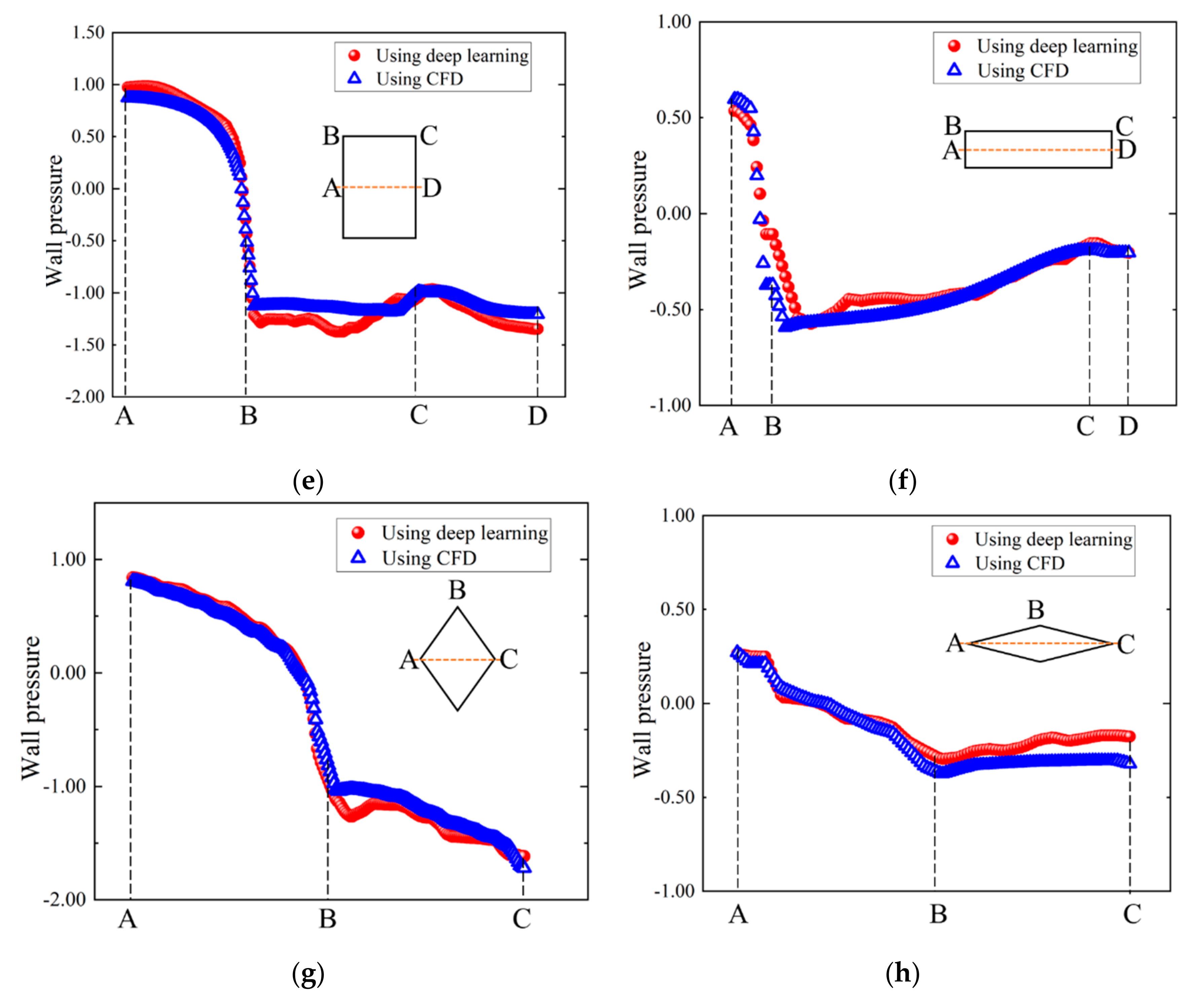
In order to avoid the problem of data heterogeneity, this paper draws on Chen’s [
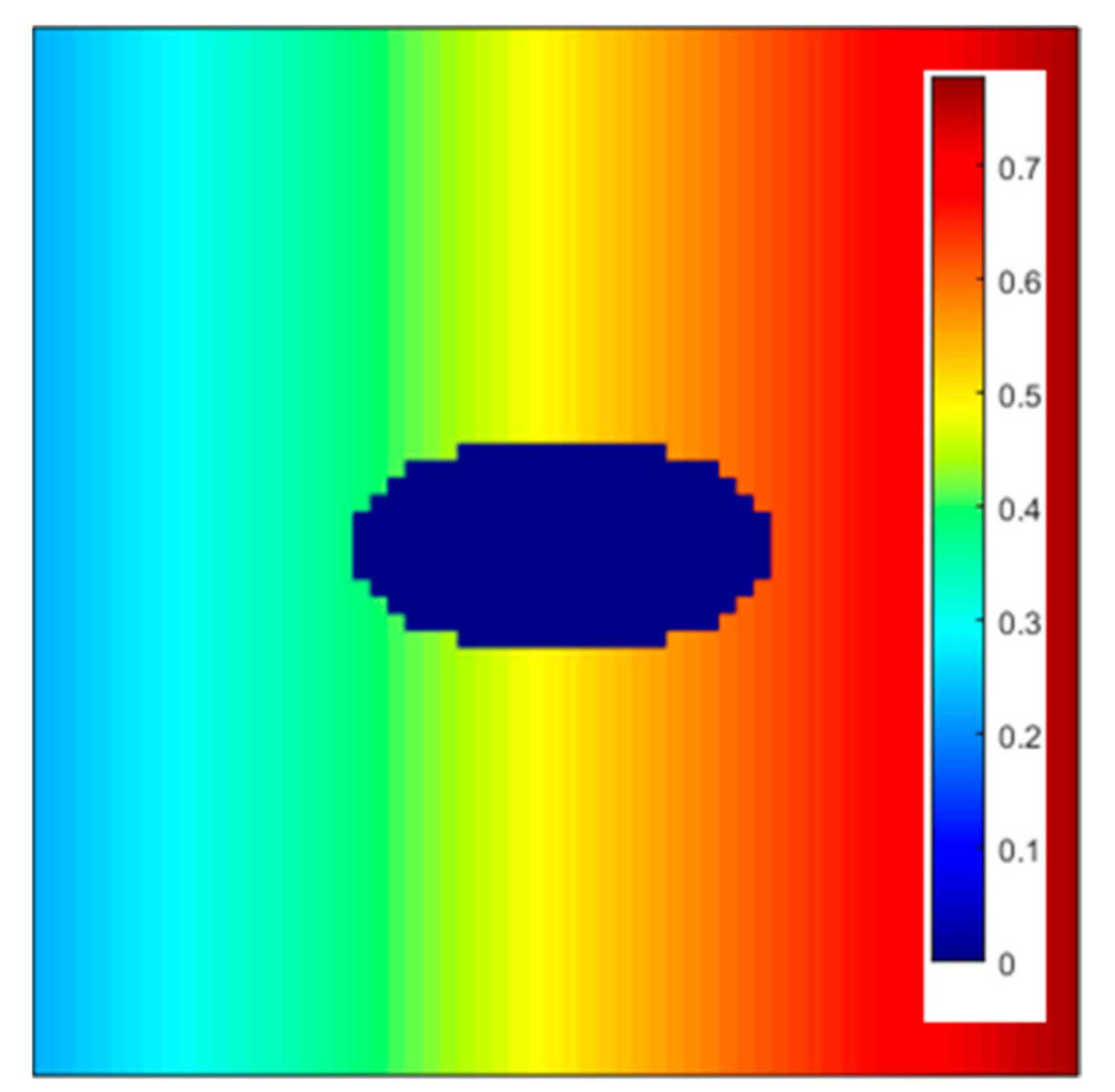
22] idea to express the shape in the form of images, that is, assigning different values to the internal and external spatial points of the shape. In Chen’s original design, the inside of the shape is expressed by 1, and the outside of the shape is expressed by 0. Although this design can express any shape, the efficiency of conveying shape information is not high, and it cannot provide the distance information of spatial points and walls. Therefore, this paper proposes the wall distance field as a description of the aerodynamic shape, which can provide the relative positional relationship between the spatial point and the wall for the limited receptive field of the CNN and directly introduce the shape pair into the input of the neural network, influencing the factors of aerostatic performance. In the wall distance field
, which is one of the model inputs (
), the assignment of the i spatial point is shown in Equation (1):
In the equation,
represents the set of distances between the i spatial point and the set of aerodynamic shape boundary points
, and
refers to the final minimum value at all distances. For the consideration of dimensionless shapes, B is introduced to represent the characteristic length of the shape. Because the space near the wall has a greater impact on the pressure field, we use a negative exponential form to increase the weight near the boundary layer while limiting the input to 1 to reduce the hidden danger of gradient explosion.
expresses the coefficient inside and outside the shape. When the i spatial point is located on the wall or inside the shape, it is set to 0, and otherwise, it is set to 1. The wall distance field
of an example ellipse with an aspect ratio of 4 is shown in
Figure 1.
2.2. Space Coordinate Field
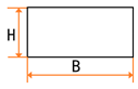
Simply using the wall distance field will result in the loss of some shape information. To illustrate this problem, the shape expressed in
Figure 2 can be taken as an example. The red frame line is the receptive field of the convolutional neural network in a hidden layer. When it moves to the two positions shown in the figure, it will receive the same wall distance field information. However, these two positions are upstream and downstream of the flow field and have different effects on the pressure field and aerostatic performance. In order to solve this problem, we also need to highlight the flow field characteristics of the aerodynamic profile of the bluff body section.
To this end, we propose to use the coordinate field describing the upstream–downstream relationship and the coordinate field describing the crosswind position as complementary information to the wall distance field as the other two inputs to the neural network.
For the coordinate field
describing the upstream-downstream relationship, the assignment of the
spatial point is shown in Equation (2):
where
represents the downwind x coordinate of the
spatial point. The origin of the x-coordinate is at the center of the section. The settings of the exponential part can achieve both the size difference between the upstream and downstream data and the normalization of the input.
Similarly, for the coordinate field
, describing the position of the crosswind direction, the assignment of the
spatial point is shown in Equation (3):
where
represents the y coordinate of the crosswind direction of the
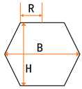
spatial point. The origin of the y-coordinate is located at the midpoint of the windward end: for circles and hexagons, it is the only windward end point, and for rectangles, it is the midpoint of the windward surface. The settings of the exponential part can achieve both the difference between the distance of the crosswind and the distance as well as the normalization of the input.
Figure 3 and
Figure 4 show the values of
and
in the spatial coordinate field for an example ellipse with an aspect ratio of 4.
3. Output Design
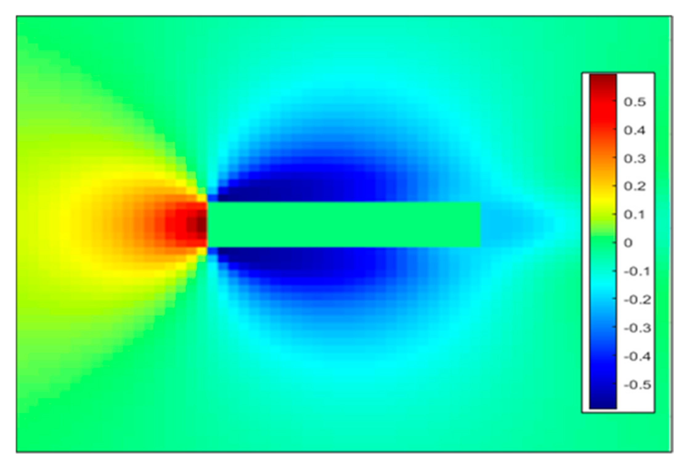
In terms of output design, the simplest and most direct approach is to use the aerostatic three-component force coefficient as the output of the prediction model. However, the mapping logic is very complicated, and it directly skips multiple data processing links such as local sampling of the pressure field and surface pressure integration. Although deep learning networks have the ability to implement the mappings, this is bound to increase the burden on the network, requiring more hidden layers and more complex structures. On the other hand, the pressure field can not only provide information on the aerostatic three-component force coefficient but also on the surrounding flow field structure, providing support for other scientific research scenarios such as flow control and heat source analysis. Therefore, this paper adopts a two-step strategy to obtain the aerostatic performance of bluff body sections. First, the neural network is used to output the pressure field
of the steady flow field, and then, the surface pressure is integrated to obtain the aerostatic three-component force coefficient.
Figure 5 shows the output of the neural network for an example rectangular section with an aspect ratio of 4.
4. Neural Network Framework Design
Convolutional neural networks have been proposed since 2012 and have achieved many application results in the fields of image classification and image detection [
23,
24]. The multi-layer convolutional structure of CNNs can automatically learn features. Shallower convolutional layers can learn some local region features, while deeper convolutional layers have larger receptive fields [
25,
26,
27]. These properties allow CNNs to learn more abstract features, and, therefore, it is widely used in image processing problems [
28]. The fully convolutional network developed on the basis of CNN is very suitable for solving the problem of mapping from image to image [
29]. FCN replaces the last fully connected layer of CNN with a convolutional layer and uses deconvolution to the last convolutional layer. The output result is unsampled, and the size of the output result is gradually restored to the same size as the input image so that a prediction value can be generated for each pixel point. The spatial information of the original input image is also preserved.
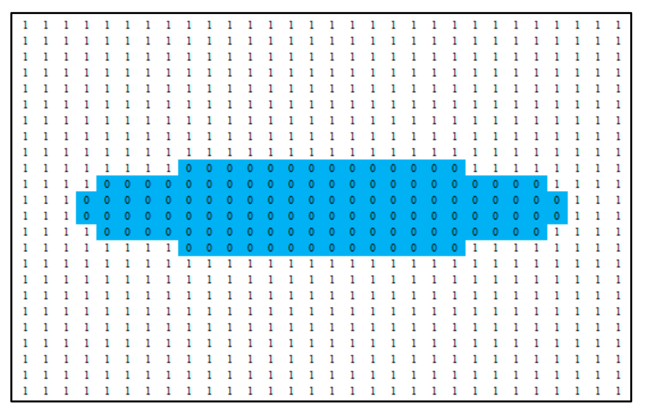
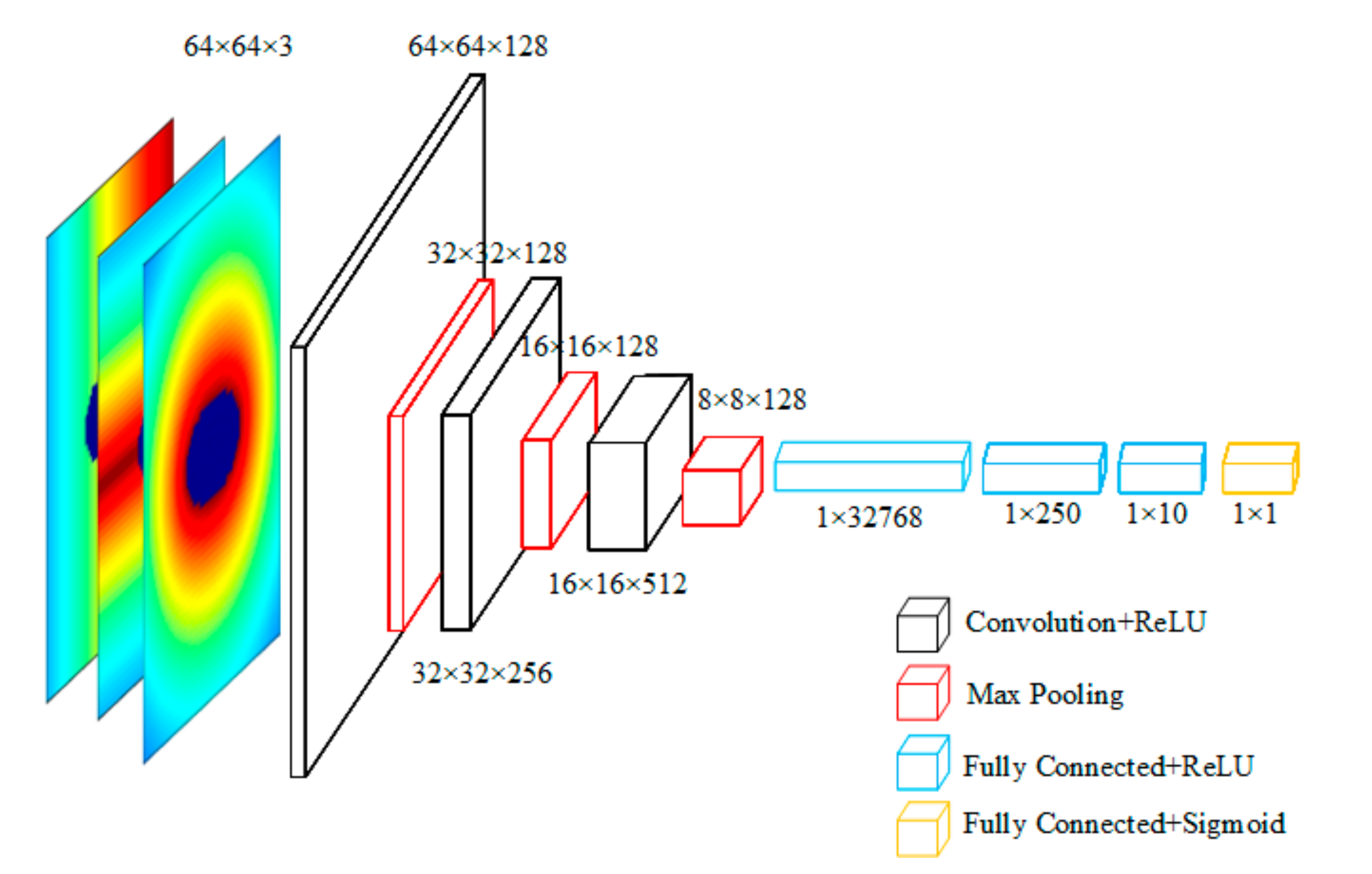
FCN is good at pixel-level classification problems, and this paper predicts the pressure field or continuous pressure value at each pixel position, which is a regression problem. Although pixel-level regression problems have higher requirements from neural network models than classification problems, they generally require training using generative neural networks. Considering that the pressure field involved in this paper has a gentle gradient and continuous smoothness, the fully convolutional network can be extended from solving pixel-level classification problems to solving pixel-level regression problems. The UNet network proposed by Ronneberger [
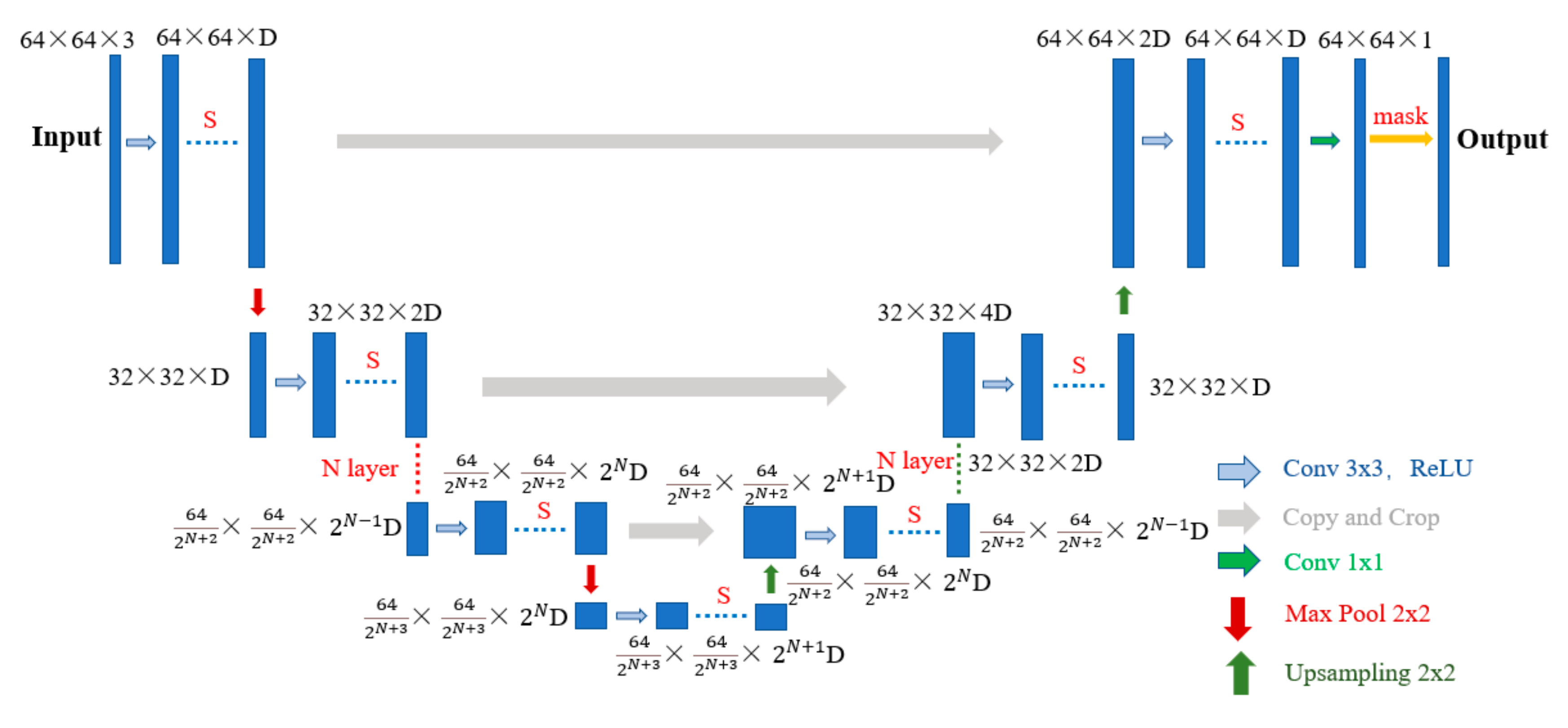
30] in 2015 can complete end-to-end training with very simple architecture, and the network inference speed is very fast, so a modified UNet network (
Figure 6) is adopted to solve the pixel-level regression problem in this paper.
Figure 6 shows the image width, height, and number of channels after convolution, pooling, and feature fusion. D represents the number of channels, S represents the number of convolutions, and N represents the number of poolings. These parameters will be studied in Chapter 6. Meanwhile, the deep learning network structure will be determined. In order to ensure that the pressure data in the aerodynamic shape is 0, a mask layer consisting of 0 and 1, with a bluff body section shape, is passed when the prediction result is output. Next, the innovative design of the UNet structure and loss value is explained.
First, the deep learning model needs to match the input and output data sizes. The input involved in this paper is the wall distance field () and the spatial coordinate field (, ), and the number of channels is 3. Considering the information content and training time contained in the image, the image pixels are set to 64 × 64. The output is a pressure field with the same size as the input image, which is a single channel picture. Since the regression problem of continuous variables needs to be predicted, it is necessary to modify the output layer of the UNet and remove the Softmax layer.
After modifying the input and output layers, the hidden layer details of the network structure are also required. The network architecture used in this paper is based on the transformation of the UNet and also consists of three parts: downsampling, upsampling, and skipping structure. The downsampling part includes the two basic components of the convolution layer and pooling layer, and the feature extraction of the input is realized by repeating the convolution-pooling process many times. The convolutional layer uses a 3 × 3 small convolution kernel, and the padding size is 1. Using max pooling makes the image twice as small after each pooling. After multiple downsamplings, the shape information of the bluff body section contained in the wall distance field and the spatial coordinate field is highly abstracted into multiple information channels, and the upsampling part is responsible for restoring the pressure field image based on this information. In order to retain more detailed information in the downsampling process, the new feature map in the upsampling process of each level and the feature map at the corresponding downsampling position are fused on the channel, which is the skip structure. In order to extract more detailed features before the final output, a 1 × 1 convolution is used to open up all information channels to achieve the regression prediction of each pixel. The convolution-pooling process is performed N times in total, and there are S convolutions each time. Both N and S will be determined in the model optimization in Chapter 6.
In the model training process, due to the different measurement standards of the classification model and the regression model, it is necessary to change the loss function used to deal with the classification problem in the original UNet network to an L2 loss function to deal with the regression error. At the same time, considering that the prediction results in this paper pay more attention to the accuracy of the flow field data around the aerodynamic shape, the L2 loss function is multiplied by the weight value. The loss value closer to the aerodynamic shape is used, with a weight value closer to 1, and for the loss value farther away from the aerodynamic shape, the weighted value is closer to 0. The weighted value of the loss function
is generated according to Equation (4):
5. Test Design
5.1. Computational Case Design
This chapter mainly shows how to obtain the data for training and verifying the model. A certain number of aerodynamic shapes are designed as an example. The shape information and the corresponding pressure field calculation results are used as the input and output of the neural network. According to different basic shapes, the calculation examples are divided into four types: regular hexagon, circle, rectangle, and regular rhombus. Each basic shape is subdivided into different shapes according to the aspect ratio and corner position, for a total of 105 shapes (
Table 1). In order to facilitate the use of a dimensionless form to determine the shape, the horizontal length of all shapes is fixed as 1 and the aerodynamic shape changes with the vertical height.
5.2. Data Preparation
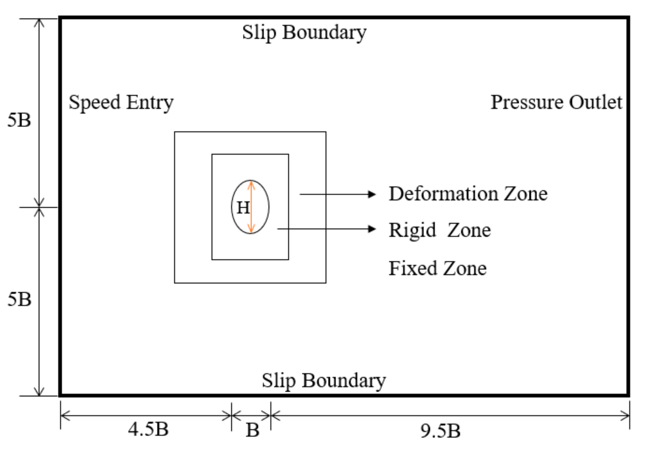
In this paper, CFD numerical simulation is used to obtain the steady-state pressure flow field of the bluff body section. The computational domain was rectangular with a blockage ratio of 0.9%. It is shown in
Figure 7, where B is the length of the bluff body section. In order to keep the mesh from changing too fast, three computational regions were defined [
31,
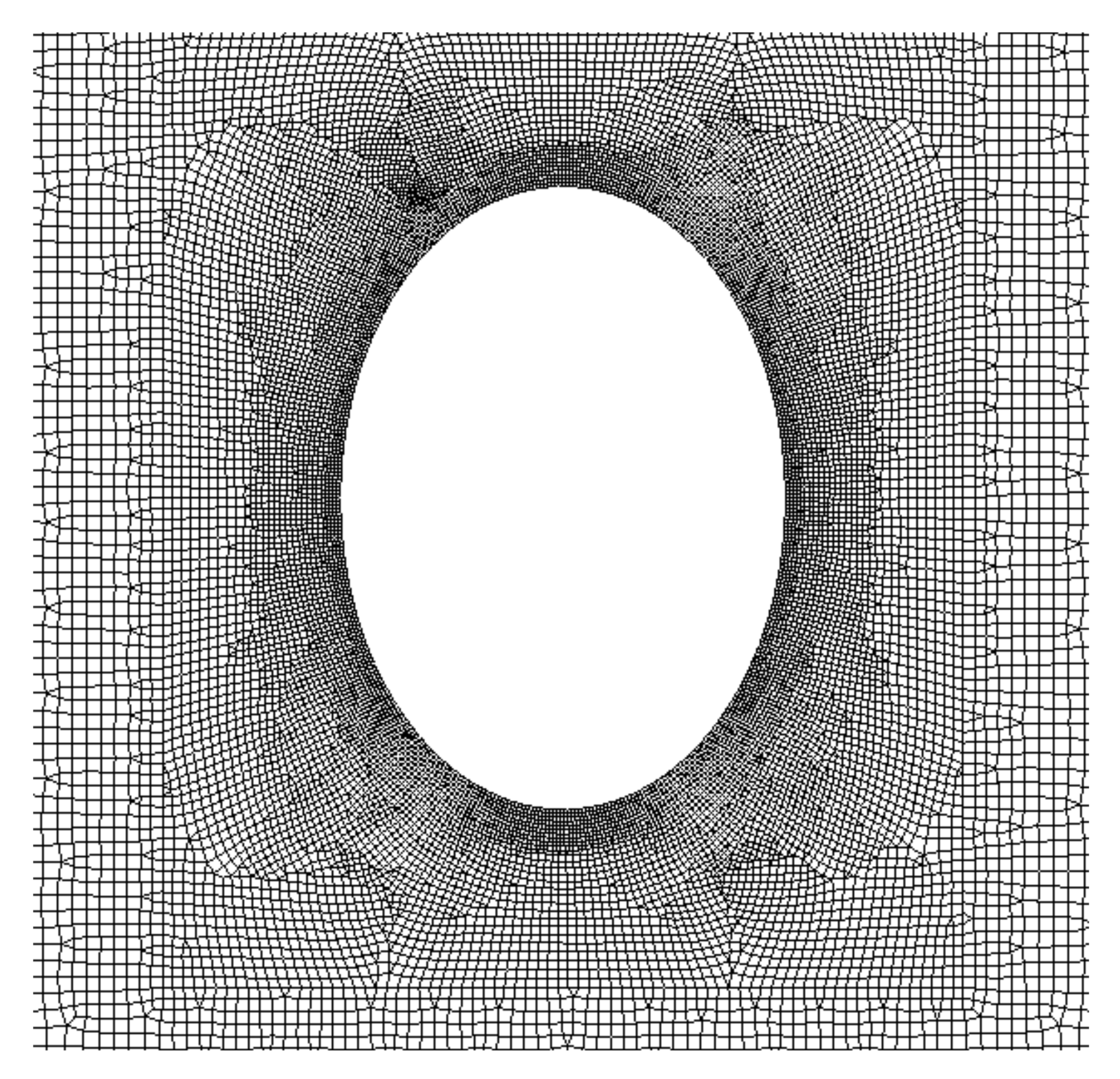
32]. The rigid zone kept the mesh shape constant, outside of which the deforming zone underwent smoothing and remeshing. The outermost fixed zone was to satisfy the blockage ratio requirement. The details of the mesh are illustrated in
Figure 8.
In order to reduce the calculation time while ensuring the calculation accuracy, the turbulence model uses the Reynolds-averaged Navier–Stokes equations (RANS). A blending k–ω SST turbulence model was used to reduce sensitivity to the inlet boundary condition. The governing momentum equation of incompressible flow is given as
where
is the two-dimensional analysis,
denotes the pressure, and
is the Reynolds stress component, in which the superscript refers to the fluctuating parts of the velocity
p. With the k–ω SST turbulence model, two additional equations are introduced to obtain the Reynolds stress component, where k is the turbulent kinetic energy and
ω is its rate of dissipation (Equations (6) and (7)). The details of the involved parameters are explained by Menter [
33]:
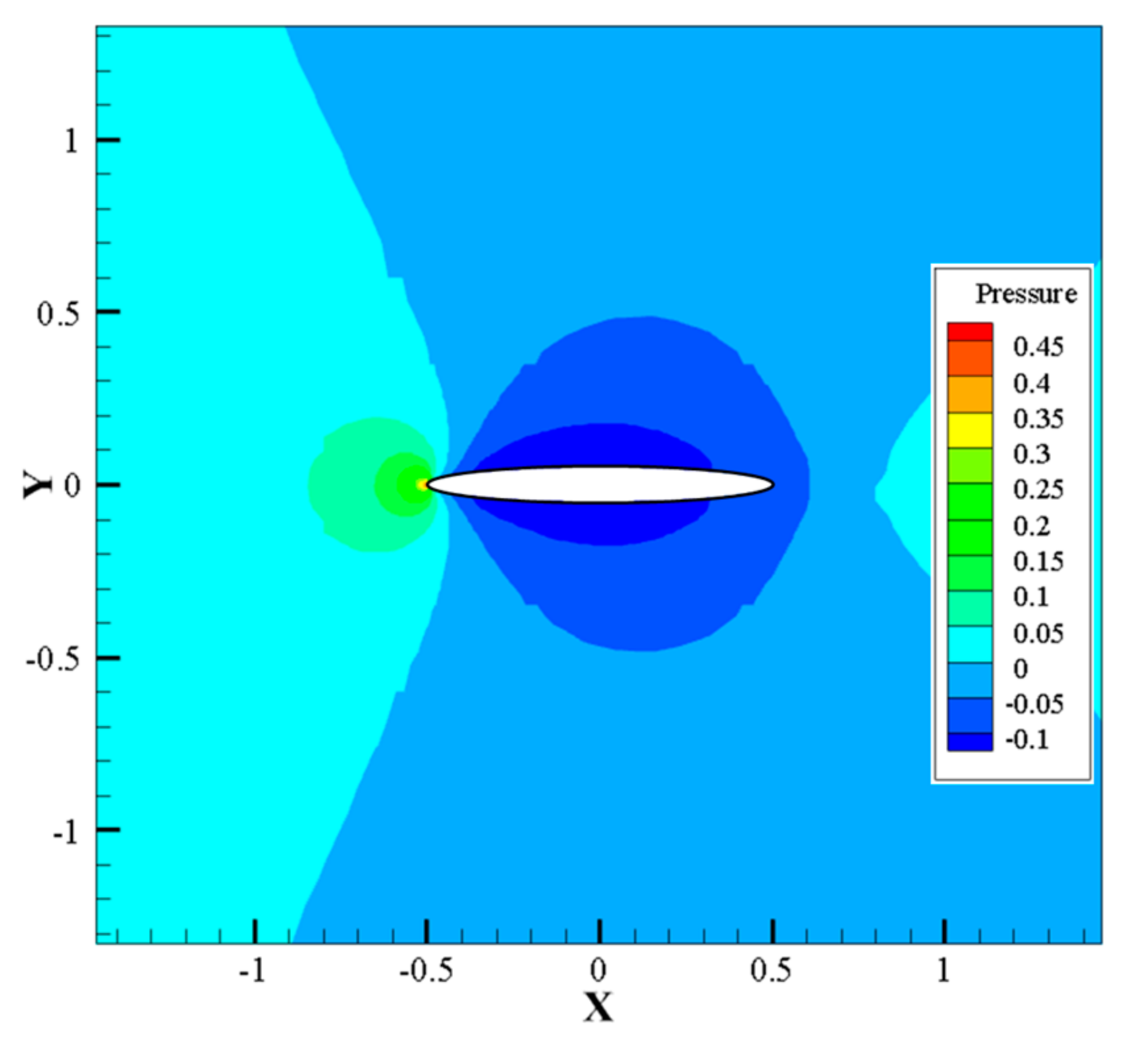
The simulations were conducted using Ansys Fluent. The semi-implicit method pressure-linked equations consistent (SIMPLEC) algorithm was used to solve the velocity–pressure coupling problem. To obtain the appropriate numerical accuracy and stability, a second-order scheme was used for the pressure equation, and the second-order upwind scheme was used for the momentum equation, turbulent kinetic energy equation, and specific dissipation rate equation. The inlet boundary was set as a velocity inlet, the incoming turbulence intensity was set as 4%, and the viscosity ratio was set as two. The outlet boundary was set as a pressure outlet. Slip conditions were applied to the top and bottom boundaries for all variables. No-slip conditions were applied to the surfaces of the bluff body section, which means that the flow state at the object’s surface was equal to the motion of the bluff body section. Considering that the section of the bluff body with a small aspect ratio in this paper is difficult to achieve the pressure field under the steady flow field when the Reynolds number is large, the Re was maintained as 4000 (using the reference length
B) in all cases. The calculation results are shown in
Figure 9.
The pressure field data is acquired once the flow field has stabilized after several iterations. Each cycle saves 10 instantaneous pressure field data, reads 5 cycles, and averages 50 instantaneous pressure field data to obtain the pressure field of the steady-state flow field. The pressure field after data processing is resampled to obtain a 64 × 64 single-channel image. The X and Y coordinates of the sampling range are [−1.26, 1.26], and the sampling size interval is 0.04. It is worth mentioning that this article mainly focuses on the construction method, so there is no need to strictly verify the accuracy of the CFD calculation results. The model training and testing are based on different data: 80% are randomly selected as the training data set, 10% are used as the validation data set, and the remaining 10% are used as the test data set. The dropout rate for the trained model is 0.2 to prevent overfitting.
6. Model Performance Evaluation and Optimization
The hyperparameters of a deep learning model directly affect the performance of the model. Taking model depth as an example, an insufficient number of hidden layers will make the model less complex and unable to capture the nonlinear mapping between input and output. However, too many hidden layers will cause unstable gradient calculations. In order to quantitatively evaluate the performance of the model, we optimize the number of channels (D), the number of convolutions (S), and the number of pooling times (N) in
Figure 6 based on the mean absolute error MAE (Equation (8)) of the extracted drag coefficient based on the predicted pressure field.
Pytorch performs very well in scientific research, which is mainly reflected in the very Pythonic style of Pytorch. Pytorch reduces the difficulty of getting started and can be built layer by layer when building a deep learning model, which is convenient for real-time modification. Therefore, this paper uses Pytorch to build the deep learning model.
6.1. Optimization of the Number of Hidden Layers
The number of hidden layers has a greater impact on the model performance than the size of the hidden layers. Therefore, this paper determines the suitable model depth for the prediction of the aerodynamic performance of the bluff body section [
34,
35]. The convolutional layer, pooling layer, and ReLU layer are considered to be downsampling components, and the number of these components (that is, the number of pooling times (N) in
Figure 6) is optimized. Considering that the size of the data image is 64 × 64, after 6 iterations of max pooling, the input information is converted into multiple channels of 1 × 1, and, therefore, the maximum number of downsampling components is set to 6. When naming the model, UNet_2-3 represents two downsampling components, and each downsampling component layer contains three convolution operations. Using the same training and validation sets, the comparison of different models is shown in
Table 2.
From the results in
Table 2, it can be seen that as the number of model layers increases, MAE first decreases, then increases, and finally decreases to its lowest value. The model obtains the smallest drag coefficient MAE when using six downsampling components. However, the data in
Table 2 are based on two convolution operations. Therefore, it is necessary to continue to observe the effect of the number of convolution operations (
Table 3).
Combining the observations in
Table 2 and
Table 3, it can be seen that when three convolutions are used, the MAE is significantly lower than when two convolutions are used. At the same time, the UNet_3-3 model has the lowest MAE and fewer parameters than the other models, and its computational cost is lower. Considering that increasing the number of convolution operations can significantly improve the model performance, in order to determine the optimal number of convolution operations for the UNet_3 model, UNet_3-4 is added for comparison. The calculation shows that the prediction result of UNet_3-4 is
and the parameter quantity is
. It can be seen that when the number of downsampling components is 3, the MAE does not decrease but increases after the number of convolution operations is increased to 4. In summary, considering the performance and the amount of computation, this paper chooses 3 as the number of downsampling components and uses the UNet network model with 3 convolutions.
6.2. Hidden Layer Size Optimization
After determining the depth of the hidden layer, it is necessary to further optimize its size, that is, the number of channels (D) in
Figure 6. The number of hidden layer channels of the first downsampling component in the selected UNet network for comparison is set to 16, 32, and 128. The number of hidden layer channels in the subsequent downsampling component is twice the model width of the previous layer. The same training set and validation set are used, and the comparison of different models is shown in
Table 4. When naming the model, UNet_3-3-16 represents that the number of hidden layer channels of the first downsampling component is 16.
It can be seen from the results in
Table 5 that as the number of hidden layer channels increases, the MAE first decreases and then increases. When the initial hidden layer channel number D is 32, the MAE is the smallest and the number of model parameters is moderate. Therefore, UNet_3-3-32 is selected for research in subsequent chapters.
7. Pressure Field Prediction Effect
The pressure field prediction accuracy directly affects the subsequent extraction of the drag coefficient, so it is necessary to check the prediction results of the flow field. After the model training is completed, the wall distance field and spatial coordinate field of the test data set are input into the model to obtain the predicted value of the pressure field. It is then converted into a visualized image and compared with the CFD calculation results, as shown in
Figure 10. Due to space limitations, representative shapes of pressure fields are selected for presentation.
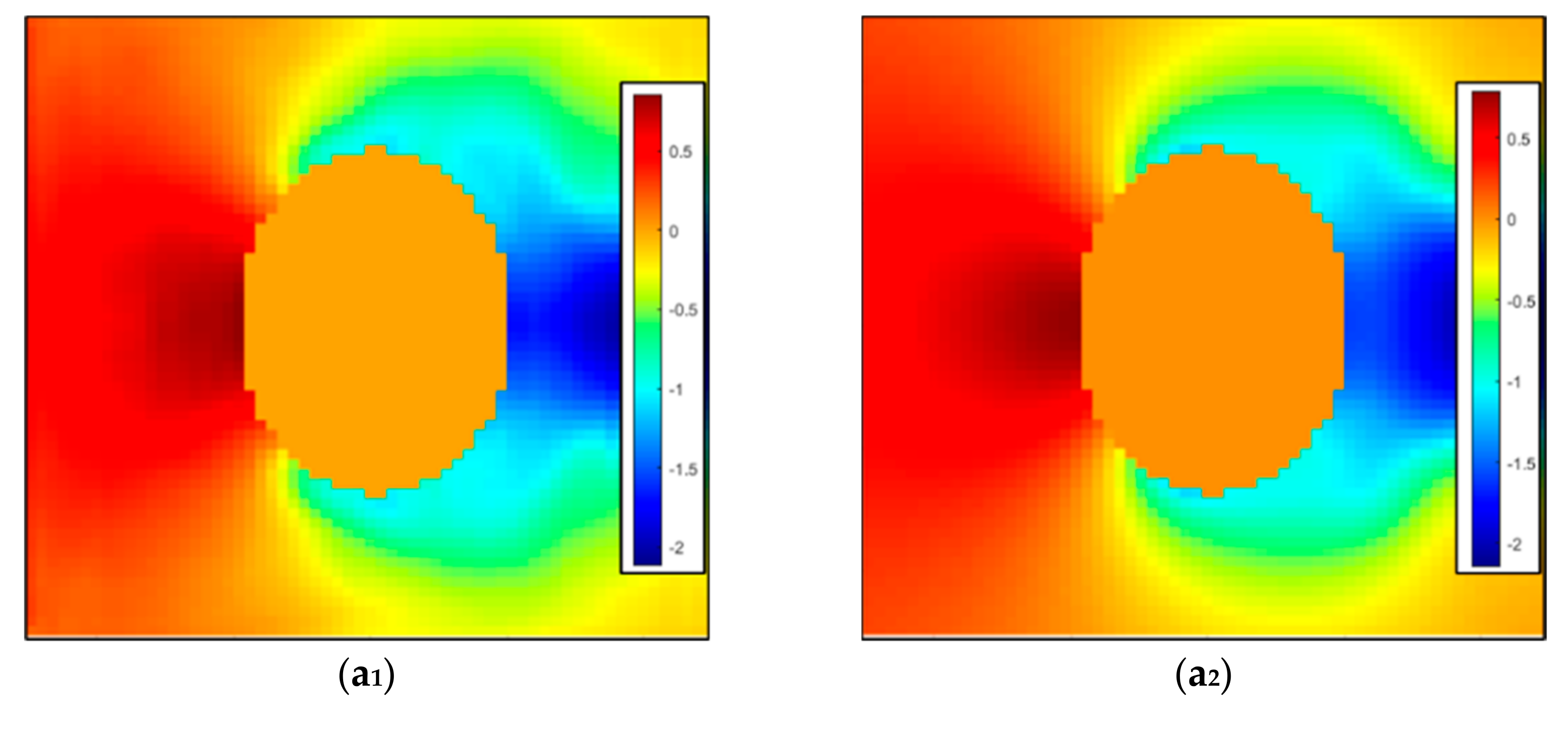
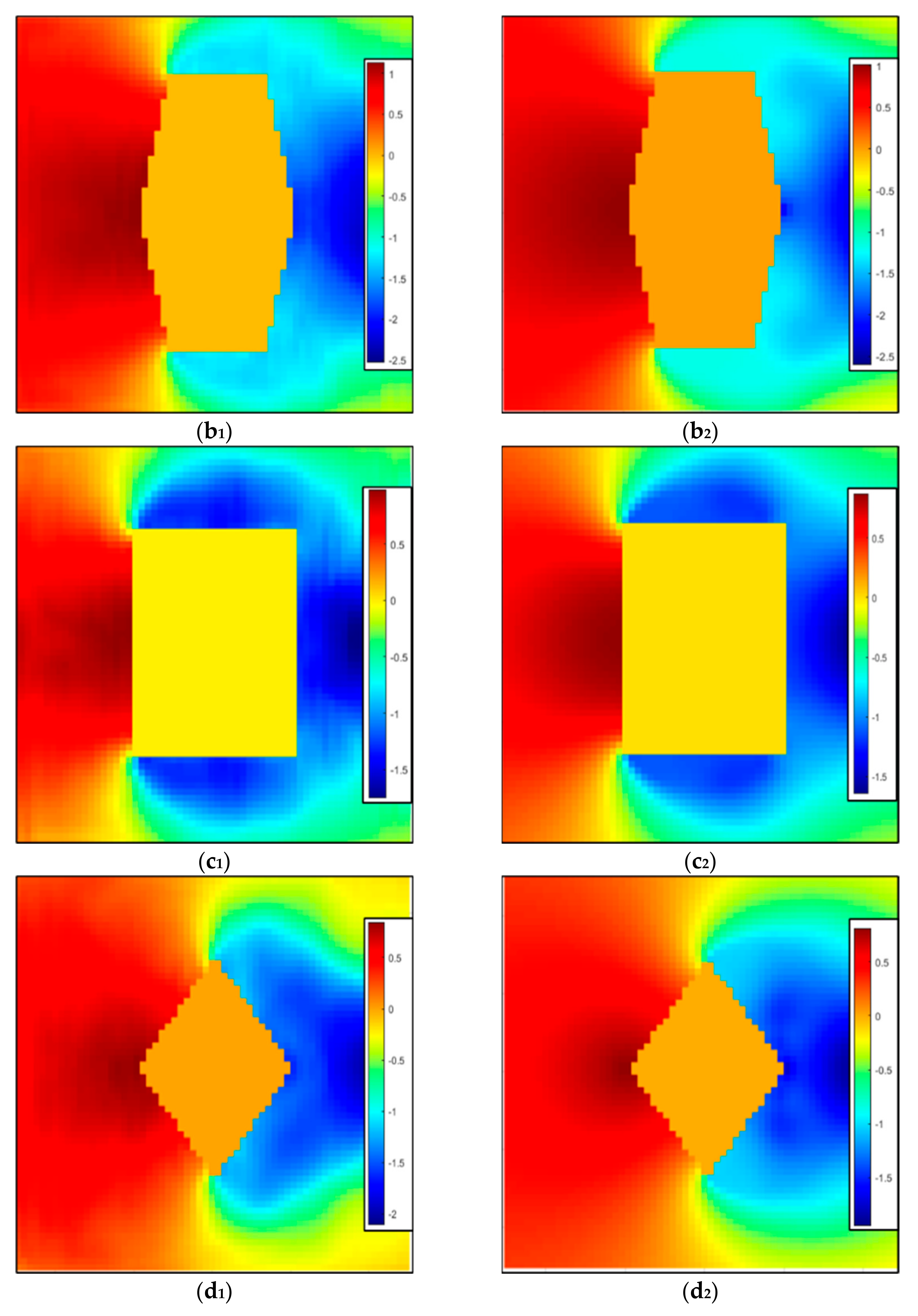
The analysis and prediction results show that the larger part of the prediction error for the ellipse, hexagon, and diamond generally exists in the negative pressure area that deviates far from the shape, and the predicted pressure is larger than the pressure field calculated by CFD. The larger part of the error of the rectangular section exists in the positive pressure area that deviates far from the shape, and the predicted pressure is smaller than that calculated by CFD. The authors believe that this phenomenon is mainly caused by two factors. First, when designing the loss function, the aerostatic performance is considered to be more closely related to the pressure field near the wall. Therefore, in order to predict the wall pressure value more accurately, the loss function gives more weight to the prediction accuracy close to the wall and has more relaxed requirements for the prediction value of the grid points farther away from the wall of the bluff body section. Secondly, the improved UNet model is still too simple, and it is necessary to use a more complex generative neural network in subsequent research. However, the improved Unet network can still achieve rapid prediction of the wall pressure and third-component force coefficient to a certain extent, as will be discussed in subsequent chapters.
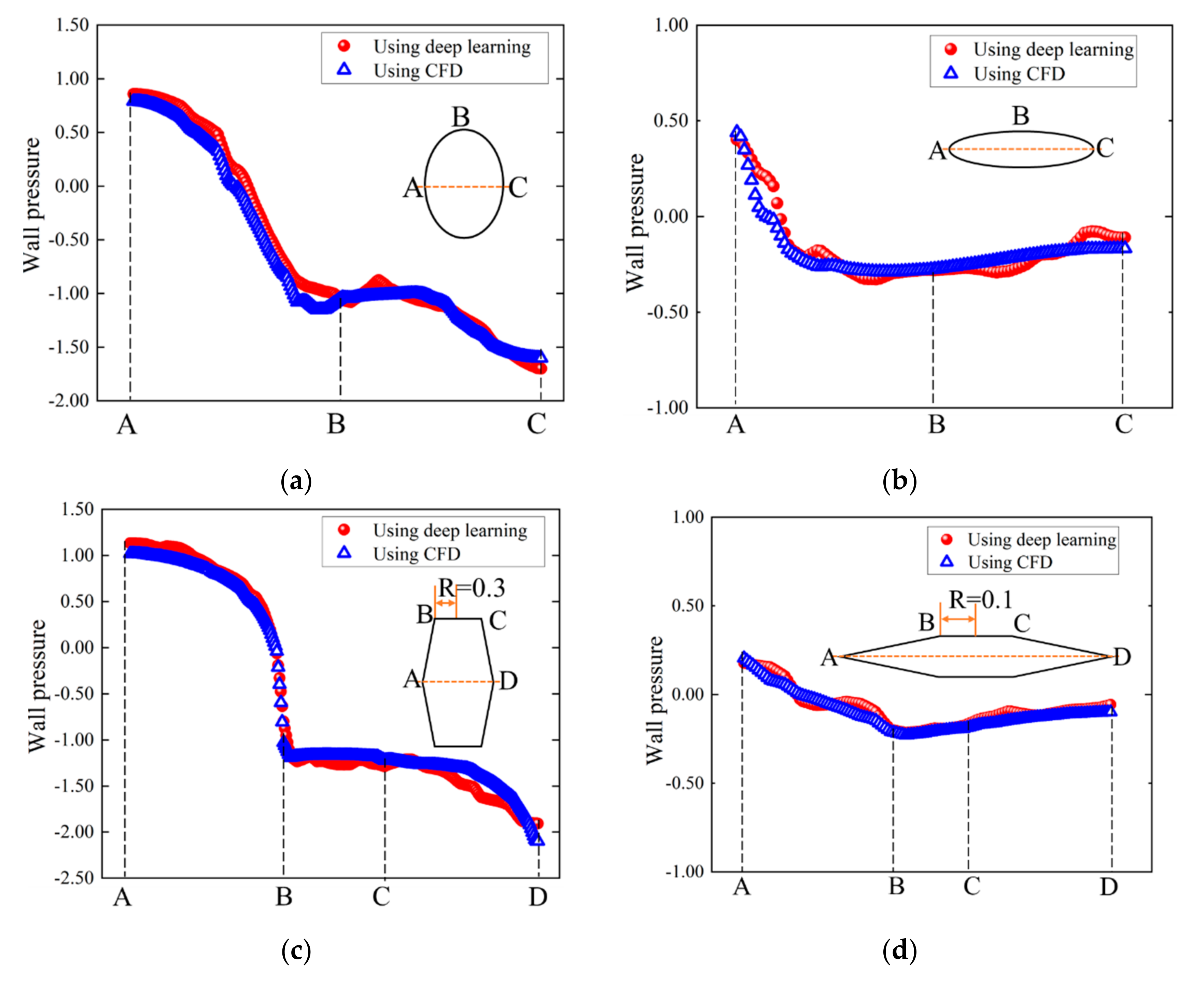
8. Wall Pressure Prediction Results
Wall pressure is of great significance in the evaluation of aerostatic performance and can also be used to extract third-component force coefficients.
Figure 11 shows the comparison of the wall pressure prediction results and the CFD calculation results. Due to space limitations, only four typical shapes and two for each shape are shown. Since the shapes used in this paper are all symmetrical up and down, only the wall pressure in the upper part is shown.
In general, the analysis of the wall pressure prediction results shows that the basic trend of the wall pressure distribution can be simulated based on the model proposed in this paper, but there are certain errors. The prediction results of the positive pressure area are generally better than those of the negative pressure area. Among them, the area with the largest error is mainly concentrated in the negative pressure area generated by flow separation and the negative pressure area near the wake. The absolute error value does not exceed 0.2 at the most, and the range is small. Meanwhile, the prediction errors of the rectangle and rhombus are generally larger than those of the ellipse and hexagon. The author believes that this is mainly caused by the uncomplicated UNet model. The original UNet model is mainly used to deal with classification problems. Although this paper has modified it, the modified UNet model still has a lot of room for improvement when dealing with regression problems.
9. Drag Coefficient Prediction
The drag coefficient under the shape can be obtained through the wall pressure of each aerodynamic shape, and the aerostatic wind load in the wind resistance design can be obtained from the drag coefficient. Therefore, the prediction of the drag coefficient is very important, and the input and output of the deep learning model also directly affect the prediction accuracy of the drag coefficient. In this paper, the three distance fields (, and ) are used as the input of the model, and the output is the pressure field. By comparing the accuracy of the drag coefficient, it is shown that the innovative input and output proposed in this paper can effectively improve the prediction accuracy.
9.1. Compared to Using Shape as Input
Donglin Chen sets the internal aerodynamic shape to 1 and the external to 0 to express the aerodynamic shape, then uses it as the model input for training. Since the sampling area in this paper is large to ensure the normal training of the model, the internal aerodynamic shape is set to 0 and the external is set to 1 to express the aerodynamic shape as the model input. In this paper, three distance fields (
,
and
) are innovatively proposed to express the aerodynamic shape and flow field information. This paper uses the UNet model determined in Chapter 6 and exactly the same parameters for training and compares the accuracy of the drag coefficient to illustrate that the three distance fields (
,
and
) proposed in this paper can effectively improve the prediction accuracy of the model. Taking an ellipse with an aspect ratio of 4 as an example, the 0–1 distance field is shown in
Figure 12. The average relative error of the drag coefficient of each basic shape predicted by the model is shown in
Table 5.
It can be seen from
Table 6 that the average relative error of the R = 0.3 hexagon reaches 45.33%, and the average relative errors of the R = 0.4 hexagon and rectangle also exceed 20%, making the total average relative error reach 22.67%. In contrast, the average relative error of the three distance fields (
,
and
) acting as the model input is 9.42%, which is 13.25% higher than the average relative error of the drag coefficient when the 0–1 distance field is used as the model input. It can be seen that the wall distance field and spatial coordinate field can make the model learn and predict more efficiently.
The average relative error when using the 0–1 distance field as the model input is much higher than the average relative error of the wall distance field and the spatial coordinate field proposed in this paper. The main reason for this is that the 0–1 distance field is too simple to express the aerodynamic shape and cannot provide effective distance information and flow field information, while the drag coefficient is closely related to the distance information and flow field information. It is, therefore, difficult for deep learning models to establish a relationship between the aerodynamic shapes and the drag coefficient.
9.2. Compared to Using the Drag Coefficient as Output
There are two ways to predict the drag coefficient of the bluff body section through the deep learning method. One is to directly predict the drag coefficient as the output; the other is to predict the pressure flow field and then pass it through the data to get the drag coefficient.
The direct method still uses the three distance fields of
,
and
as the input of the model and the processed drag coefficient as the output. The CNN model consists of the convolutional layer, pooling layer, ReLU layer, and fully connected layer. The CNN model, with a model depth of 3 layers and an initial model width of 128, was selected by comparing the size of the MAE and the number of parameters, as shown in
Figure 13.
By directly predicting the drag coefficient through the CNN model, the overall average relative error of the test set reached 19.64%, the average relative error of the diamond reached 38.81%, and the average relative errors of the R = 0.2 regular hexagon and the R = 0.3 regular hexagon were less than 10%.
The author believes there are two main reasons for the large error in the direct prediction of the drag coefficient through the CNN model. The first reason is that there are very obvious differences between the basic shapes, which makes it difficult to accurately associate the shape input with the drag coefficient in the deep learning model. Therefore, we can only fit relatively satisfactory results under different shapes, which leads to large errors in some shapes. The second reason is that it is too simplistic to directly use the drag coefficient data as the output and directly use the image as the output. When predicting a number such as a drag coefficient, it is difficult for a deep learning model to establish a certain connection between the input and output. The randomness is also large, which makes the model prediction less stable.
In reference to the first reason, better deep learning model architecture can be selected by changing the structure of the model. However, the CNN model is the optimal solution for the direct prediction of the drag coefficient in this paper. Therefore, the output needs to be redesigned for the second reason. The drag coefficient can be obtained indirectly by predicting the pressure field of the steady-state flow field. The input of the model is still the three distance fields of
,
and
and the output is the stable pressure flow field. Due to the different input and output models, the UNet network is selected and the optimal model is determined, as shown in
Figure 6.
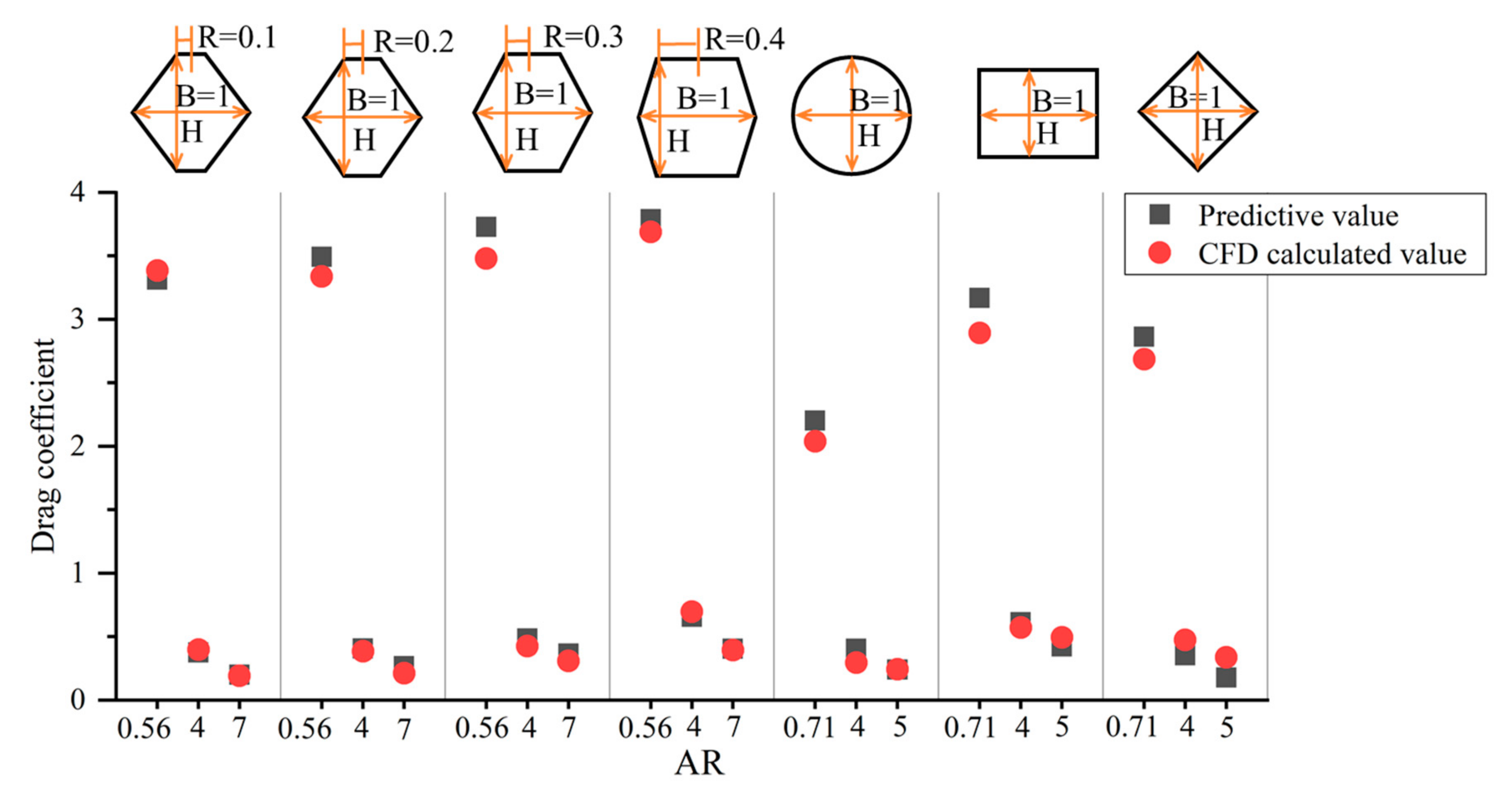
Considering that the drag coefficients of different shapes are quite different, the average relative error is used to comprehensively evaluate the prediction accuracy of different shapes, as shown in
Table 6. At the same time, the comparison between the predicted drag coefficient and the CFD-calculated drag coefficient for each shape is shown in
Figure 14.
From the prediction results given in
Table 6, it can be seen that the average relative errors of the drag coefficients of the R = 0.1 hexagon, R = 0.2 hexagon, and R = 0.4 hexagon and circle are less than 10%. A direct relationship is maintained between the accuracy of the wall pressure prediction and the prediction accuracy of the drag coefficient. The relative errors of the drag coefficients predicted by the R = 0.3 hexagon, rectangle, and diamond exceed 10% but do not exceed 20%. The average relative error is the largest for the diamond, reaching 15.42%. The average relative error for all shapes is 9.42%. It can be seen that the UNet model adopted by the indirect method has better performance than the CNN model that directly predicts the drag coefficient, and the average relative error of the drag coefficient is increased by 10.22%. It can be seen that the indirect method of predicting the drag coefficient strengthens the connection between the input and the output. The prediction of the flow field can also provide applications for flow field control and other scenarios, and the practical performance of the model is greatly improved.
10. Conclusions
This paper proposes a novel, fully convolutional neural network model that enables rapid prediction from shape to aerostatic performance.
- (1)
The overall average relative error of the drag coefficient is 9.42%.
- (2)
The shape is described by the combination of the wall distance field and the space coordinate field. This improves the prediction accuracy by 13.25% compared to when the shape is directly used as the model input.
- (3)
A step-by-step strategy in which the pressure field is used as the model output is proposed. The model prediction accuracy is improved by 10.22% when using the pressure field as the model input compared to directly predicting the drag coefficient.
Author Contributions
Conceptualization, K.L.; methodology, K.L.; software, H.L.; validation, H.L.; formal analysis, H.L.; investigation, K.L.; resources, K.L.; data curation, Z.C.; writing—original draft preparation, H.L.; writing—review and editing, K.L.; visualization, H.L.; supervision, S.L.; project administration, S.L.; funding acquisition, K.L. and S.L. All authors have read and agreed to the published version of the manuscript.
Funding
This research was funded by the National Science Foundation for Young Scientists of China grant number 51808075; the National Science Foundation of China grant number 51978108, the 111 project of the Ministry of Education and the Bureau of Foreign Experts of China grant number B18062; the Natural Science Foundation of Chongqing China grant number cstc2020jcyj-msxmX0773 and cstc2020jcyj-msxmX0937; the Fundamental Research Funds for the Central Universities grant number 2020CDJ-LHZZ-018, 2021CDJQY-025 and 2020CDJ-LHZZ-016; the Chongqing full-time postdoctoral exit and stay in the Chongqing Project grant number 2020LY07.
Institutional Review Board Statement
Not applicable.
Informed Consent Statement
Not applicable.
Data Availability Statement
Not applicable.
Acknowledgments
This paper is supported by the National Science Foundation of China (51808075, 51978108), 111 Project (B18062), the Natural Science Foundation of Chongqing, China (cstc2020jcyj-msxmX0773, cstc2020jcyj-msxmX0937), the Fundamental Research Funds for the Central Universities (2020CDJ-LHZZ-018, 2021CDJQY-025 and 2020CDJ-LHZZ-016), and the Chongqing full-time postdoctoral exit and stay in the Chongqing Project (2020LY07).
Conflicts of Interest
The authors declare no conflict of interest.
References
- Matsuda, K.; Tokushige, M.; Iwasaki, T. Reynolds number effects on the steady and unsteady aerodynamic forces acting on the bridge deck sections of long-span suspension bridge. IHI Eng. Rev. 2007, 40, 12. [Google Scholar]
- Simiu, E.; Scanlan, R.H. Wind Effects on Structures: Fundamentals and Applications to Design; John Wiley: New York, NY, USA, 1996. [Google Scholar]
- Shimada, K.; Ishihara, T. Prediction of aeroelastic vibration of rectangular cylinders by K-e model. J. Aerosp. Eng. 1999, 12, 122–135. [Google Scholar] [CrossRef]
- Liu, S.Y.; Zhao, L.; Fang, G.S.; Hu, C.; Ge, Y.J. Investigation on aerodynamic force nonlinear evolution for a central-slotted box girder under torsional vortex-induced vibration. J. Fluids Struct. 2021, 106, 103380. [Google Scholar] [CrossRef]
- Chen, W.-L.; Li, H.; Hu, H. An experimental study on the unsteady vortices and turbulent flow structures around twin-box-girder bridge deck models with different gap ratios. J. Wind Eng. Ind. Aerodyn. 2014, 132, 27–36. [Google Scholar] [CrossRef]
- Chen, W.-L.; Zhang, Q.-Q.; Li, H.; Hui, L. An experimental investigation on vortex induced vibration of a flexible inclined cable under a shear flow. J. Fluids Struct. 2015, 54, 297–311. [Google Scholar] [CrossRef]
- Laima, S.; Li, H.; Chen, W.-L.; Li, F. Investigation and control of vortex-induced vibration of twin box girders. J. Fluids Struct. 2013, 39, 205–221. [Google Scholar] [CrossRef]
- Mannini, C.; Sbragi, G.; Schewe, G. Analysis of self-excited forces for a box-girder bridge deck through unsteady RANS simulations. J. Fluids Struct. 2016, 63, 57–76. [Google Scholar] [CrossRef]
- Xu, F.Y.; Wu, T.; Ying, X.Y.; Kareem, A. Higher-order self-excited drag forces on bridge decks. J. Eng. Mech. 2016, 142, 06015007. [Google Scholar] [CrossRef]
- Li, H.; Chen, W.-L.; Xu, F.; Li, F.-C.; Ou, J.-P. A numerical and experimental hybrid approach for the investigation of aerodynamic forces on stay cables suffering from rain-wind induced vibration. J. Fluids Struct. 2010, 26, 1195–1215. [Google Scholar] [CrossRef]
- Hongye, G.; Biao, Y.; Hui, H.; Rui, X.; Chang, L.; Yu, L.; Qianhui, P. State-of-the-art review of bridge informatization and intelligent bridge in 2019. J. Civ. Environ. Eng. 2020, 4, 14–27. [Google Scholar]
- Lute, V.; Upadhyay, A.; Singh, K. Support vector machine based aerodynamic analysis of cable stayed bridges. Adv. Eng. Softw. 2009, 40, 830–835. [Google Scholar] [CrossRef]
- Jung, S.; Ghaboussi, J.; Kwon, S.-D. Estimation of aeroelastic parameters of bridge decks using neural networks. J. Eng. Mech. 2004, 130, 1356–1364. [Google Scholar] [CrossRef]
- Liao, H. Machine learning strategy for predicting flutter performance of streamlined box girders. J. Wind Eng. Ind. Aerodyn. 2021, 209, 104493. [Google Scholar] [CrossRef]
- Hu, G.; Kwok, K. Predicting wind pressures around circular cylinders using machine learning techniques. J. Wind Eng. Ind. Aerodyn. 2020, 198, 104099. [Google Scholar] [CrossRef]
- Hu, G. Deep learning-based investigation of wind pressures on tall building under interference effects. J. Wind Eng. Ind. Aerodyn. 2020, 201, 104138. [Google Scholar] [CrossRef]
- Guo, X.; Li, W.; Iorio, F. Convolutional Neural Networks for Steady Flow Approximation. In Proceedings of the 22nd ACM SIGKDD International Conference on Knowledge Discovery and Data Mining, San Francisco, CA, USA, 13–17 August 2016; pp. 481–490. [Google Scholar]
- Miyanawala, T.P.; Jaiman, R.K. A Novel Deep Learning Method for the Predictions of Current Forces on Bluff Bodies. In Proceedings of the ASME 2018 37th International Conference on Ocean, Offshore and Arctic Engineering, Madrid, Spain, 17–22 June 2018. [Google Scholar]
- Jin, X.; Cheng, P.; Chen, W.-L.; Wen-Li, C. Prediction model of velocity field around circular cylinder over various Reynolds numbers by fusion convolutional neural networks based on pressure on the cylinder. Phys. Fluids 2018, 30, 47–105. [Google Scholar] [CrossRef]
- Lee, S.; You, D. Data-driven prediction of unsteady flow over a circlular cylinder using deep learning. J. Fluid Mech. 2019, 879, 218–254. [Google Scholar] [CrossRef] [Green Version]
- Ribeiro, M.D.; Rehman, A.; Ahmed, S.; Dengel, A. DeepCFD: Efficient Steady-State Laminar Flow Approximation with Deep Convolutional Neural Networks. arXiv 2020, arXiv:2004.08826. [Google Scholar]
- Chen, D.; Gao, X.; Xu, C.; Chen, S.; Fang, J.; Wang, Z. FlowGAN: A Conditional Generative Adversarial Network for Flow Prediction in Various Conditions. In Proceedings of the 32nd International Conference on Tools with Artificial Intelligence (ICTAI 2020), Baltimore, MD, USA, 9–11 November 2020. [Google Scholar]
- Sermanet, P.; Eigen, D.; Zhang, X.; Mathieu, M.; Fergus, R.; LeCun, Y. OverFeat: Integrated Recognition, Localization and Detection using Convolutional Networks. arXiv 2013, arXiv:1312.6229. [Google Scholar]
- He, K. Spatial Pyramid Pooling in Deep Convolutional Networks for Visual Recognition. IEEE Trans. Pattern Anal. Mach. Intell. 2015, 37, 1904–1916. [Google Scholar] [CrossRef] [Green Version]
- Szegedy, C.; Liu, W.; Jia, Y.; Sermanet, P.; Reed, S.; Anguelov, D.; Erhan, D.; Vanhoucke, V.; Rabinovich, A. Going Deeper with Convolutions. In Proceedings of the IEEE Conference on Computer Vision and Pattern Recognition, Columbus, OH, USA, 23–28 June 2014. [Google Scholar]
- Dan, C.; Alessandro, G.; Luca, G.; Jürgen, S. Deep Neural Networks Segment Neuronal Membranes in Electron Microscopy Images. Adv. Neural Inf. Process. Syst. 2012, 25, 2852–2860. [Google Scholar]
- Zeiler, M.D.; Fergus, R. Visualizing and Understanding Convolutional Networks. In European Conference on Computer Vision, Proceedings of the Computer Vision–ECCV 2014, Zurich, Switzerland, 6–12 September 2014; Springer: Cham, Switzerland, 2014; pp. 818–833. [Google Scholar]
- Girshick, R.; Donahue, J.; Darrell, T.; Malik, J. Region-Based Convolutional Networks for Accurate Object Detection and Segmentation. IEEE Trans. Pattern Anal. Mach. Intell. 2015, 38, 142–158. [Google Scholar] [CrossRef]
- Shelhamer, E.; Long, J. Fully Convolutional Networks for Semantic Segmentation. IEEE Trans. Pattern Anal. Mach. Intell. 2017, 39, 640–651. [Google Scholar] [CrossRef] [PubMed]
- Ronneberger, O.; Fischer, P.; Brox, T. U-Net: Convolutional networks for biomedical image segmentation. In Medical Image Computing and Computer-Assisted Intervention 2015, Proceedings of the Medical Image Computing and Computer-Assisted Intervention–MICCAI 2015, 18th International Conference, Munich, Germany, 5–9 October 2015; Navab, N., Hornegger, J., Wells, W.M., Frangi, A.F., Eds.; Springer International Publishing: Cham, Switzerland, 2015; pp. 234–241. [Google Scholar]
- Miranda, S.D.; Patruno, L.; Ubertini, F.; Vairo, G. On the identification of flutter derivatives of bridge decks via RANS turbulence models: Benchmarking on rectangular prisms. Eng. Struct. 2014, 76, 359–370. [Google Scholar] [CrossRef]
- Patruno, L. Accuracy of numerically evaluated flutter derivatives of bridge deck sections using RANS: Effects on the flutter onset velocity. Eng. Struct. 2015, 89, 49–65. [Google Scholar] [CrossRef]
- Menter, F.R. Zonal two equation k-omega turbulence models for aero-dynamic ows. In Proceedings of the 24th Fluid Dynamics Conference, Orlando, FL, USA, 6–9 July 1993. [Google Scholar]
- Eldan, R.; Shamir, O. The Power of Depth for Feedforward Neural Networks. In Proceedings of the Conference on Learning Theory, New York, NY, USA, 23–26 June 2016; pp. 907–940. [Google Scholar]
- Lu, Z.; Pu, H.; Wang, F.; Hu, Z.; Wang, L. The Expressive Power of Neural Networks: A View from the Width. In Proceedings of the Advances in Neural Information Processing Systems 30 (NIPS 2017), Long Beach, CA, USA, 4–9 December 2017. [Google Scholar]
Figure 1.
Wall distance field of an ellipse with AR = 4.
Figure 1.
Wall distance field of an ellipse with AR = 4.
Figure 2.
Relationship between receptive field and shape.
Figure 2.
Relationship between receptive field and shape.
Figure 3.
field of an ellipse with AR = 4.
Figure 3.
field of an ellipse with AR = 4.
Figure 4.
field of an ellipse with AR = 4.
Figure 4.
field of an ellipse with AR = 4.
Figure 5.
Pressure field of a rectangular section with AR = 4.
Figure 5.
Pressure field of a rectangular section with AR = 4.
Figure 6.
Modified UNet network structure.
Figure 6.
Modified UNet network structure.
Figure 7.
Sketch of the two-dimensional (2D) computational domain.
Figure 7.
Sketch of the two-dimensional (2D) computational domain.
Figure 8.
Detailed demonstration of the computational grid within the rigid zone.
Figure 8.
Detailed demonstration of the computational grid within the rigid zone.
Figure 9.
CFD calculation of pressure cloud map.
Figure 9.
CFD calculation of pressure cloud map.
Figure 10.
Comparison of pressure field prediction effects of four typical shapes. The first column is the predicted value. (a1) The ellipse with AR = 0.71. (b1) The hexagon with AR = 0.56 R = 0.3. (c1) The rectangle with AR = 0.71. (d1) The diamond with AR = 0.71. The second column is the true value. (a2) The ellipse with AR = 0.71. (b2) The hexagon with AR = 0.56 R = 0.3. (c2) The rectangle with AR = 0.71. (d2) The diamond with AR = 0.71.
Figure 11.
Comparison of the prediction effects of the wall pressure field of the four shapes. (a) The ellipse with AR = 0.71. (b) The ellipse with AR = 4. (c) The hexagon with AR = 0.56 R = 0.3. (d) The hexagon with AR = 7 R = 0.1. (e) The rectangle with AR = 0.71. (f) The rectangle with AR = 4. (g) The diamond with AR = 0.71. (h) The diamond with AR = 4.
Figure 12.
Partial 0–1 distance field.
Figure 12.
Partial 0–1 distance field.
Figure 13.
Determined CNN model.
Figure 13.
Determined CNN model.
Figure 14.
Drag coefficient prediction results.
Figure 14.
Drag coefficient prediction results.
Table 1.
List of the shape conditions.
Table 1.
List of the shape conditions.
| Basic shape | ![Applsci 12 03147 i001]() | ![Applsci 12 03147 i002]() | ![Applsci 12 03147 i003]() | ![Applsci 12 03147 i004]() |
| Distance R from upper corner to X = 0 | [0.1, 0.2, 0.3, 0.4] | — | — | — |
| B | 1 |
| AR = B/H | [0.5, 0.56, 0.625, 0.71, 0.83, 1, 2, 3, 4, 5, 6, 7, 8, 9, 10] |
| Quantity | 60 | 15 | 15 | 15 |
Table 2.
Model performance comparison—number of downsampling components.
Table 2.
Model performance comparison—number of downsampling components.
| Model Settings | UNet_2-2 | UNet_3-2 | UNet_4-2 | UNet_5-2 | UNet_6-2 |
|---|
| MAE | 0.2313 | 0.2038 | 0.1942 | 0.2190 | 0.1593 |
| Parameter quantity | 1.016 × 10⁶ | 4.262 × 10⁶ | 1.724 × 10⁷ | 6.915 × 10⁷ | 2.768 × 10⁸ |
Table 3.
Model performance comparison—number of convolutions.
Table 3.
Model performance comparison—number of convolutions.
| Model Settings | UNet_2-3 | UNet_3-3 | UNet_4-3 | UNet_5-3 | UNet_6-3 |
|---|
| MAE | 0.1801 | 0.1175 | 0.1696 | 0.1456 | 0.1234 |
| Parameter quantity | 1.533 × 10⁶ | 6.401 × 10⁶ | 2.587 × 10⁷ | 1.037 × 10⁸ | 4.152 × 10⁸ |
Table 4.
Model performance comparison—number of convolutions.
Table 4.
Model performance comparison—number of convolutions.
| Model Settings | UNet_3-3-16 | UNet_3-3-32 | UNet_3-3-64 | UNet_3-3-128 |
|---|
| MAE | 0.1531 | 0.0942 | 0.1175 | 0.1700 |
| Parameter quantity | 4.010 × 10⁵ | 1.601 × 10⁶ | 6.401 × 10⁶ | 2.559 × 10⁷ |
Table 5.
Average relative error of predicted drag coefficient after changing input.
Table 5.
Average relative error of predicted drag coefficient after changing input.
| Shape | R = 0.1
Hexagon | R = 0.2
Hexagon | R = 0.3
Hexagon | R = 0.4
Hexagon | Circle | Rectangle | Diamond |
|---|
| Average relative error (%) | 7.690 | 22.20 | 45.33 | 26.72 | 17.26 | 21.37 | 18.13 |
Table 6.
Average relative error of predicted drag coefficient after changing output.
Table 6.
Average relative error of predicted drag coefficient after changing output.
| Shape | R = 0.1
Hexagon | R = 0.2
Hexagon | R = 0.3
Hexagon | R = 0.4
Hexagon | Circle | Rectangle | Diamond |
|---|
| Average relative error (%) | 3.450 | 7.740 | 12.14 | 5.010 | 9.110 | 13.08 | 15.42 |
| Publisher’s Note: MDPI stays neutral with regard to jurisdictional claims in published maps and institutional affiliations. |
© 2022 by the authors. Licensee MDPI, Basel, Switzerland. This article is an open access article distributed under the terms and conditions of the Creative Commons Attribution (CC BY) license (https://creativecommons.org/licenses/by/4.0/).


