Effect of Topography Truncation on Experimental Simulation of Flow over Complex Terrain

Featured Application

This article analyzes the effect of topography truncation on wind characteristics of flow over complex terrain in a wind tunnel simulation.

Abstract

Wind tunnel tests are a commonly used method for studying wind characteristics of complex terrain; but truncation of the terrain model is usually unavoidable and affects the accuracy of the test results. For this reason, the effects of truncated and original terrain models on the simulation of wind characteristics for complex terrain were investigated by considering both nontruncated and truncated models, with the truncated model considering the applicability of two types of transition sections. The results show that the effect of topographic truncation on profiles of mean velocity and turbulence intensity is different for regions and that inclination angle profiles are extremely sensitive to the changing topographic features upwind. In those cases, the spectra of streamwise velocity were overestimated in the low-frequency range but underestimated in the high-frequency range due to topographic truncation. At the same time, the less negative value of the slope of the spectra was found at the inertial subrange. Furthermore, the normalized bandwidth was also influenced by topographic truncation, which was narrowed in windward and leeward regions and broadened in the valley region. We should note that the performance of the transition sections used in this study was quite limited and even resulted in inaccuracies in the simulation.

1. Introduction

Flow over complex terrain remains a formidable issue that plays an important role in many practical applications, including wind power micrositing, pollution dispersion as well as wind loading on bridges and transmission towers. Flow separation and reattachment regions induced by topographies such as ridges, cliffs and escarpments not only lead to misconceptions about flow characteristics but also cause difficulties in wind tunnel testing and numerical simulation. Flow characteristics in a region close to a topographic feature and to what extent the flow is influenced by the terrain geometry are not exactly specific [1]. An in-depth understanding of complex turbulent flows is essential for greatly improving simulation accuracy, especially for numerical simulations including the large eddy simulation (LES) and the unsteady Reynolds-averaged Navier-Stokes (URANS). Significant effort has been devoted in recent years to gaining a better understanding of flow characteristics in complex terrains with wind tunnel testing [2,3,4,5,6]. Furthermore, numerical simulation can be compared to validate results [7]. Kilpatrick et al. [8] investigated the effect of inflow conditions on the characteristics of flow over Bolund Hill. Bolund Hill is a well-studied test case for wind power misting and numerical simulations, as its steep geometry poses a challenge for numerical models to resolve [9]. Lange et al. [10] studied the mean flow behavior and turbulence intensity when flowing over Bolund Hill under a round or sharp escarpment leading edge; wind energy production was also analyzed. To further study the unsteady flow behavior around Bolund Hill, a 1/115 scale model was employed in the wind tunnel experiment by Yeow et al. [11]. Several field measurements had also been carried out to verify the experimental and numerical models [12,13,14]. In addition, early studies such as Askervein Hill [15] and Kettles Hill [16] are classic cases for studying the characteristics of flow over complex terrain.

The above-mentioned studies primarily focused on terrains such as regular independent hills, slopes and steep escarpments to reveal the mechanism of the flow over different terrains. There was little attention devoted to real complex terrains where the topography and geometry are more intricate. Due to the limitations of the wind tunnel test and of the numerical computational domain, complex terrain models should be truncated. The bottom of a terrain model is determined by the lowest elevation in the real terrain. Because the elevation differences of real topography such as deep-cutting gorges and valleys are often extreme, the edges of the model are higher than the bottom side of the wind tunnel and computational domain. This phenomenon, named “artificial cliff” [17], leads to flow separation and baffling flow at the leading edge, changing inflow conditions and inaccuracies in the test. Several methods have been proposed to address the “artificial cliff”[18,19,20]. For example, a transition section, which was used to connect the floor of the wind tunnel or numerical computational domain and the terrain model edge, was proposed to avert flow separation. There are various forms of transition sections, such as ramps, bicubic transition curves, and Witoszynski transition curves. Jubayer and Hangan [21] implemented 3.2 mm thick masonite sheets at the model front and sides to smoothen the height transition from the wind tunnel floor to the model edge. Maurizi et al. [22] used a ramp transition section with a slope of 5.7° to simulate the wind characteristics of a mountainous terrain by numerical simulation. Although the form of the ramp transition section is simple and easy to use, its applicability still needs to be verified. For topography with large elevation differences, the length of the ramp transition section may be too long to be suitable for a wind tunnel simulation because of the limitation of the test section. Moreover, the slope of the ramp transition section should be small, otherwise flow separation and baffling flow will still occur. Accordingly, the ramp transition section is not applicable for highly undulating topography. In this case, Hu et al. [23] proposed a theoretical curve based on the potential flow theory around the cylinder and then conducted a performance comparison between the theoretical curve and ramp transition. For application convenience, Hu et al. [24] simplified the expression of the theoretical curve based on the original. Huang et al. [17] proposed a comprehensive method to evaluate the performance of several curve transitions including the Hu et al. [24] improved theoretical curve. Chen et al. [25] considered different weights of speed-up factors, wind attack angle, and turbulence intensity by combining a weighted solution based on the correlation degree to ameliorate the evaluation method for determining the optimal form of the transition section.

Although transition sections are widely implemented in experiments and numerical simulations, the feasibility is still difficult to explain, because neither wind tunnel nor numerical simulations can avoid “artificial cliff”. Additionally, comprehensively detailed field measurement data of flow over complex terrain, which is time-consuming and highly expensive, are also difficult to obtain. Hence, analyzing the effect of the transition section on flow characteristics is not possible. Nevertheless, based on previous studies on wind tunnel simulations of intricate topographic flows, the details of terrain models play an important role [10,26,27]. In the study of Lange et al. [10], the variation in the escarpment leading edge, which had round or sharp geometry, generated completely different flow behavior on the rear. The difference in annual energy production estimated based on the two scenarios differed from 20% to 51%. Furthermore, the structural dynamic response and aerodynamic characteristics are highly sensitive to changes in the flow characteristics [28,29,30,31]. Accordingly, a systematic study is needed to evaluate the effect of topographic truncation on flow over complex terrain.

Based on the above reasons, a wind tunnel simulation of flow over intricate terrain was conducted to obtain wind characteristics and analyze the effect of topographic truncation. The terrain model was scaled from an isolated island, which is the optimum simulation object to avoid the “artificial cliff” because the transition between island topography and sea level is smooth. Flow over complex terrain was investigated by assessing how changes to the forms of transition sections, including the original topography, affect flow behavior at different measurement locations. The flow parameters investigated included mean velocity, inclination angle, turbulence intensity, and velocity spectra.

2. Experimental Method

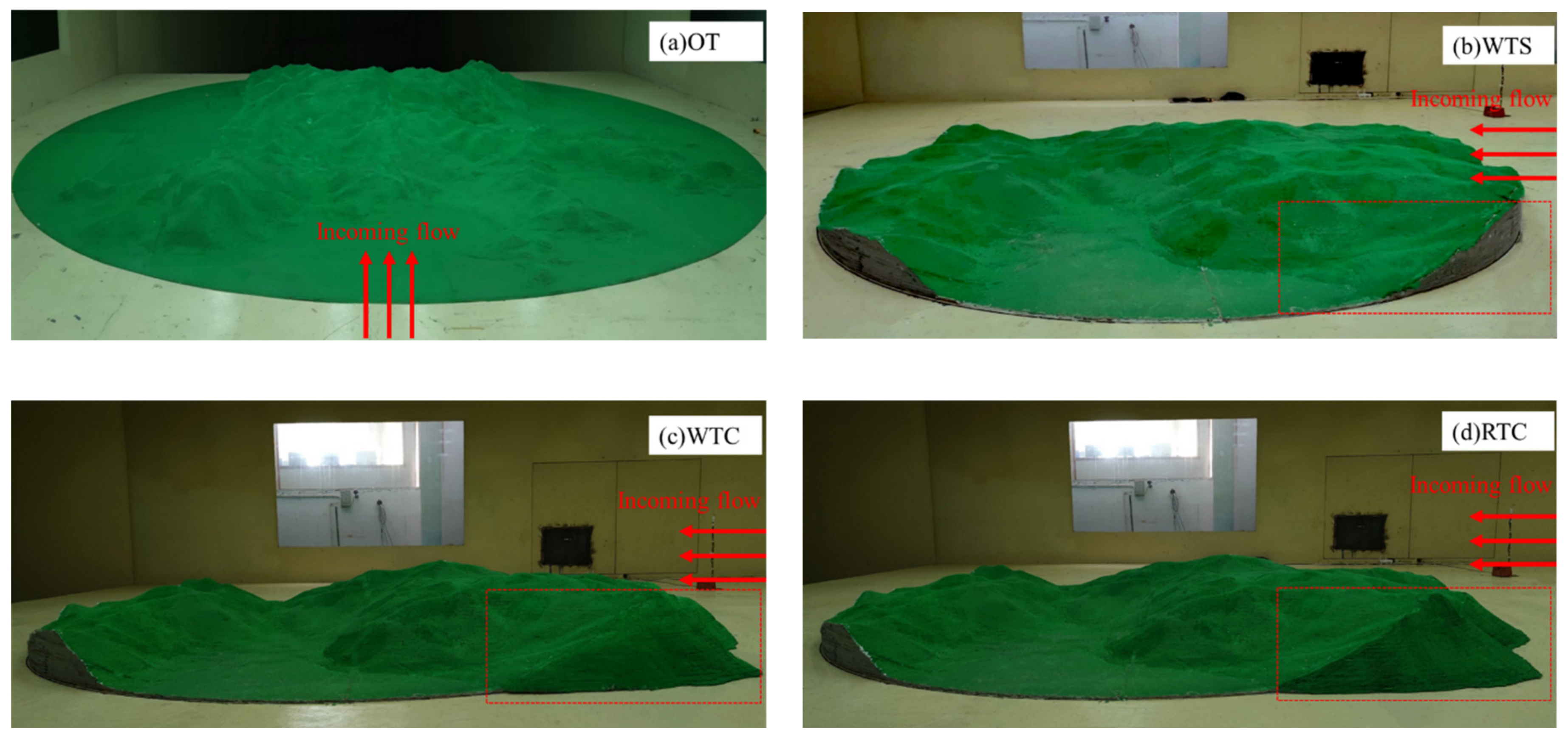
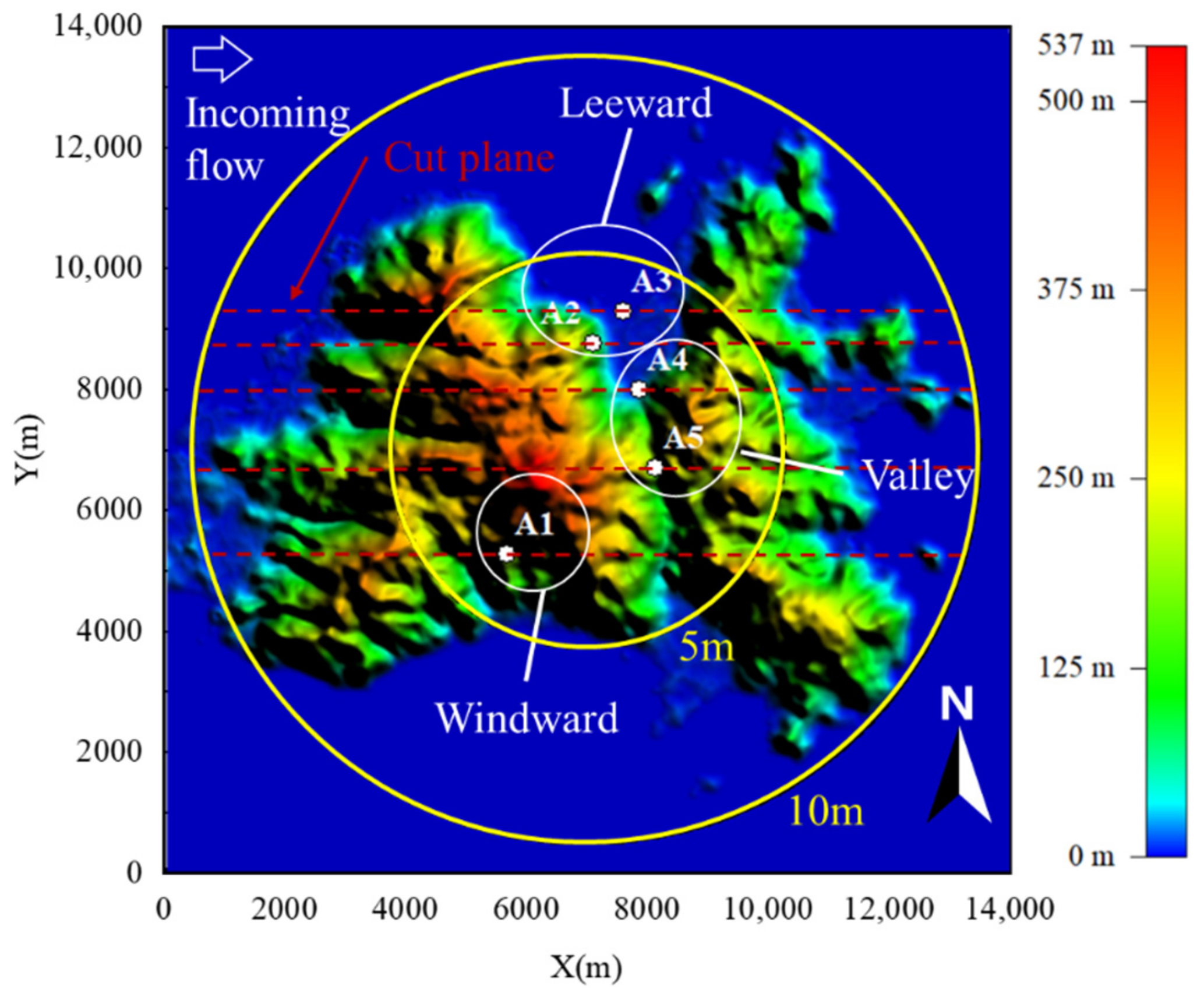
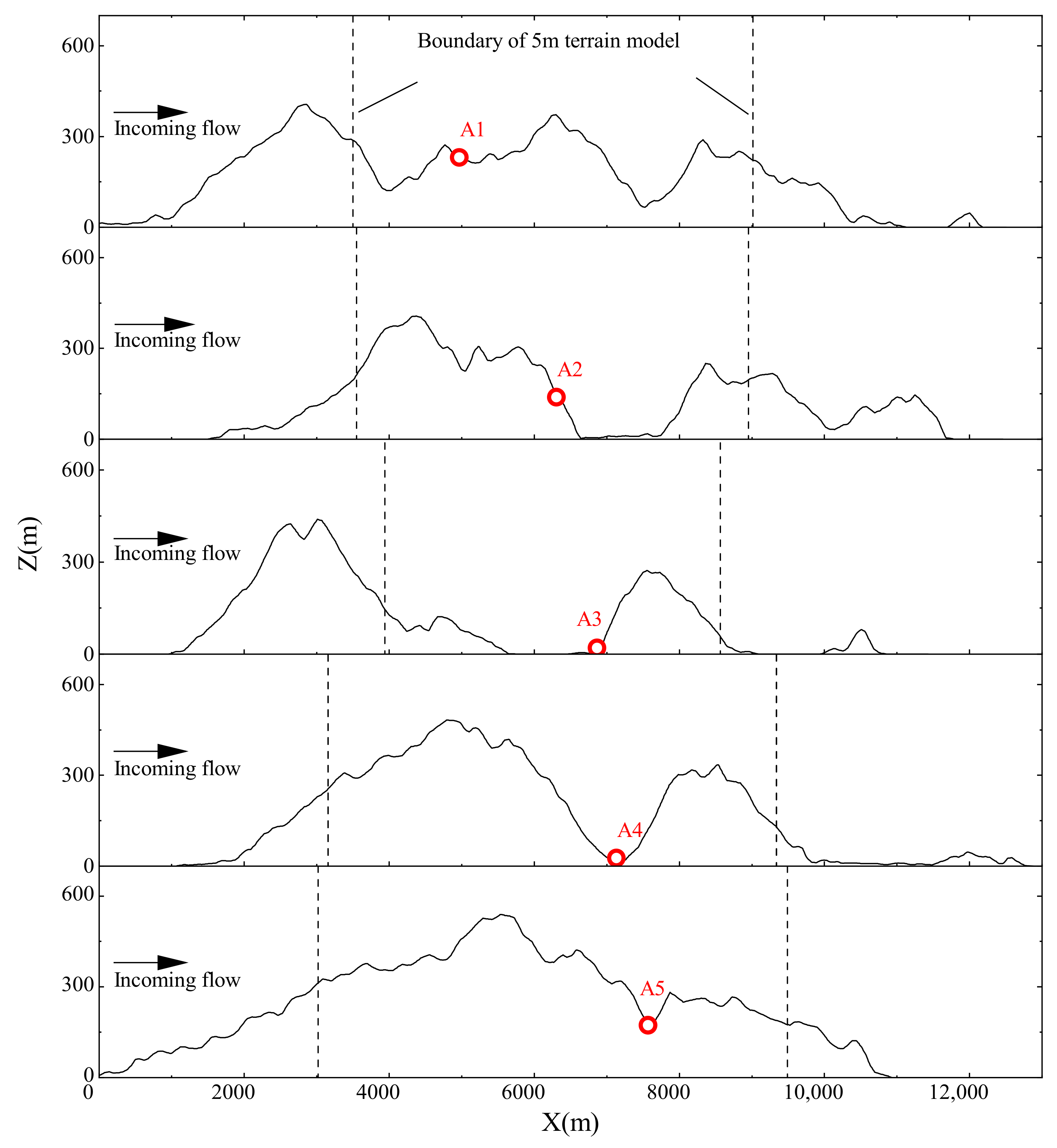
2.1. Terrain Scale Model

The topography investigated herein is an island located in the coastal region of South China. A view of this region is shown in Figure 1 along with the measurement locations for this study. For the wind tunnel test, wind speeds were measured at a total of five locations on the island, which are potential wind power sites. The center region of the island has the highest elevation with a mountain running northwest to southeast. There is a valley to the east of the mountain with another mountain stretching from the northeast to the southwest to the east of the valley. Overall, the topography of the island can be characterized as high-west and low-east. According to the topographic features of the island and the incoming flow direction, measurement locations were divided into three regions: windward region, leeward region, and valley region. As shown in Figure 1, location A1 was situated in the windward region, which is the windward slope of the center mountain, while locations A2 and A3 were situated at the leeward slope. The valley region representing the valley terrain at the island center included measurement locations of A4 and A5.

For the wind tunnel testing, a 1:1300 scale terrain model was made of polyethylene foam and overlapped layer by layer according to the terrain contour line. The scale ratio was much larger than the ratio of 1:5000 recommended by Bowen [32] to avoid the error of turbulence viscous dissipation. The diameter of the test terrain model was 10 m for the full island model and 5 m for the truncation model with a maximum height of 0.41 m. The covered area of the terrain model was different according to the model diameter. The large one covered an area of approximately 132.7 km², and the small one covered an area approximately one-fourth the size of the larger one. The terrain of the full island is shown in Figure 1, and two circles indicate the areas covered by the terrain model with diameters of 10 m and 5 m. The blockage ratio was approximately 3.27% for the terrain model with a diameter of 10 m, which is lower than the maximum allowable blockage ratio of 5% recommended by Holmes [33].

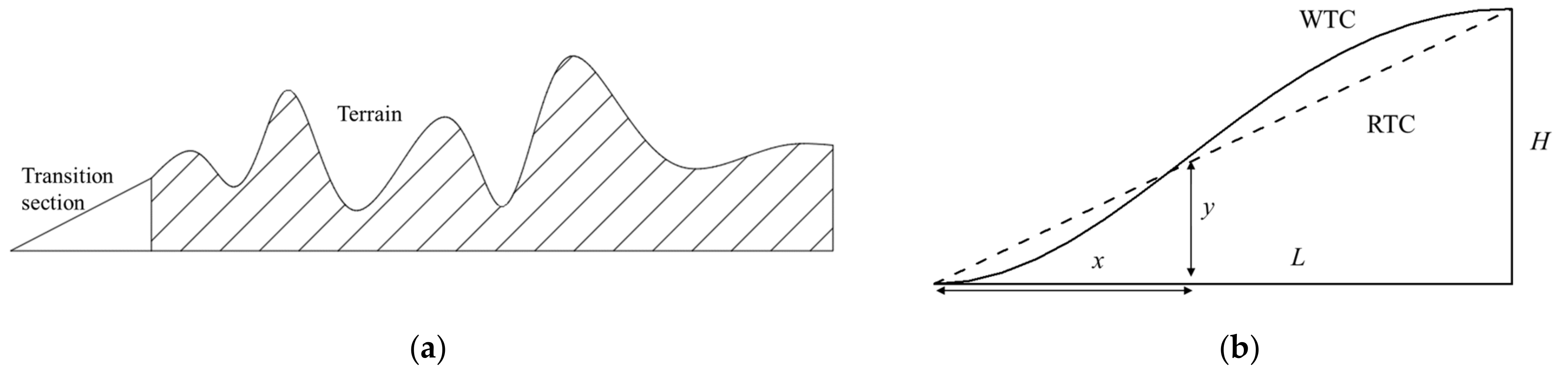
2.2. Transition Sections

The transition section connecting the wind tunnel floor or the bottom of the numerical computational domain was proposed to handle the “artificial cliff” generated by topographic truncation, as shown in Figure 2a. This idea was inspired by the contraction curve of the wind tunnel, which can achieve good flow quality and avoid flow separation.

Four cases conducted in this study are shown in Figure 3: original topography (OT), without transition section (WTS), Witozinsky transition curve (WTC), and ramp transition curve (RTC). According to previous studies [17,23,24,25], the performance of the transition curve was evaluated by comparing the characteristics of the flow after the transition section with incoming flow, and the less differences observed, the better. However, the studies of Kilpatrick et al. [1] and Lange et al. [10] highlighted the significant effect of the leading edge geometry of the terrain model on the flow behavior over the Bolund Hill. The implementation of a transition section to smooth the altitude difference between the model edge and the wind tunnel floor may change the leading-edge geometry, but the degree to which the flow is influenced is not completely understood. Furthermore, when transition sections were applied in the complex terrain, flow characteristics observed at measurement locations were affected not only by transition sections but also by complex terrain. Hence, it is not appropriate to evaluate the performance of transition sections by comparing flow characteristics with incoming flow. For this purpose, the test case with original topography was carried out as criterion instead of incoming flow, and the case without transition sections and the one with two forms of transition sections were also conducted in this study for comparison. Figure 2b shows a sketch of these two transition curves. The first one is the WTC, which is widely applied in low-speed wind tunnels. The formula of WTC can be described as follows:

$$y=H\left\{1-\frac{{\left[1-{\left(x/L\right)}^2\right]}^2}{{\left[1+\alpha {(x/L)}^2\right]}^3}\right\}$$

(1)

where α = 50, H is the altitude difference between the model edge and the wind tunnel floor, and L is the length of the transition curve at certain points corresponding to H to maintain the equivalent slope H/L = 0.5774. The other is RTC with the same slope but a straight line for the transition curve.

2.3. Experimential Set-Up

The testing facility was the wind tunnel laboratory of Central South University, which is a closed-circuit atmospheric boundary layer wind tunnel with two test sections. The test was carried out in the low-speed section with a width of 12 m and a height of 3.5 m. The test wind speed was set to 10 m/s with a uniform profile. The incoming flow came from the west to the island, which is the most critical wind direction based on the local meteorological statistics. Furthermore, the altitude difference caused by topographic truncation is most obvious on the west side due to the high-west and low-east topography of the island. The Reynolds numbers based on model height h can be calculated as Re = U h/ν, where U is the streamwise velocity and ν = 1.47 × 10⁻⁵ m²/s is the kinematic viscosity of air at 20 °C. The value of Reynolds numbers in this study was approximately 3.0 × 10⁵, which is in the range of 1.7 × 10⁵–4.6 × 10⁵ studied by Kilpatrick et al. [1]. According to their research, the flow behavior is generally less affected by the Reynolds number. For the other nondimensional numbers determining the flow similarity between the wind tunnel and the real island, the Richardson number and the Eckert number similarities were satisfied due to the consideration of the neutrally stratified boundary layer, and the Prandtl number similarity was satisfied by the air working fluid. Depending on the early study of flow over complex terrain [34], the Rossby similarity was relaxed because of the practical difficulties of modeling the Coriolis force in the wind tunnel. The Froude similarity was also relaxed, because no thermal stratification was reproduced in the wind tunnel.

A turbulence flow instrument cobra probe with a high-frequency up-to 10 kHz and measurement accuracy within ±0.5 m/s was used to measure the velocity at different locations on the terrain model. In this study, the data were sampled at 2 kHz. A minilaser range finder with measurement accuracy within ±1 mm was used to measure the distance above the ground.

3. Mean wind Characteristics

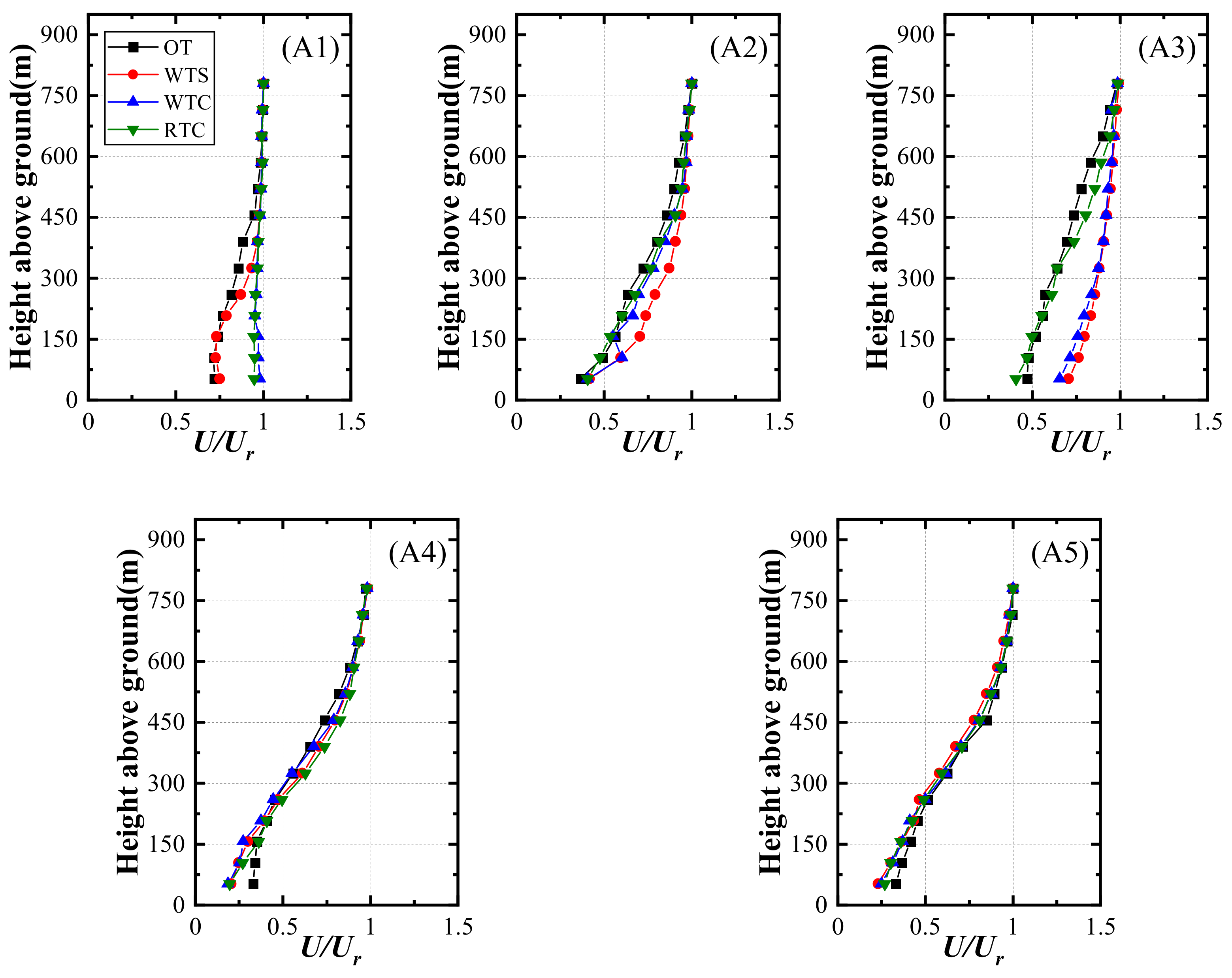
3.1. Mean Velocity

Profiles of streamwise velocity U, which were normalized by the mean velocity at the top height of each location U_r to reduce the influence of variation in incoming flow velocity, are shown in Figure 4 for four test cases with uniform inflow conditions but different forms of the transition section. For the convenience of analysis and interpretation, Figure 5 provides east-west cutting planes of measurement locations.

Figure 4 shows the normalized velocity profiles of location A1, where obvious differences in the four test cases are found near the ground. The influenced area is approximately 450 m above the ground in true magnitude, in which the profiles of WTC and RTC are higher than the other two. Because A1 sits at the windward of the center mountain near the edge of the terrain model, the speed-up effects generated by transition sections control this area. For OT and WTS, the mean velocity profiles are similar under a height of approximately 400 m. However, it should be noted that the flow behaviors in these two cases are completely different. In case OT, there is a side mountain range running northeast to southwest at the front of location A1. As shown in Figure 5, the mountain peak lies ahead of location A1 with a height of approximately 400 m, leading to a blockage effect and flow separation. Hence, the mean velocity profile in the OT case shows a smaller speed at the part below approximately 400 m. In addition, for the case WTS, the front mountain peak was truncated and created an “artificial cliff” with a height of 287 m. Owing to the larger height difference between the terrain model edge and the wind tunnel floor, separation bubbles occurred, and flow separation controlled this region. However, this does not mean that the WTS shows better performance than the WTC and RTC. It is just a special case with a mountain peak at the front of location A1. Moreover, both the WTC and RTC could accelerate the flow near the ground. When the transition section is implemented, the speed-up effect should be considered, which may considerably affect the experimental accuracy, especially for the locations close to the terrain model leading edge.

The leeward region, which includes locations A2 and A3, is on the downhill slope to the leeward of the peak. These locations are located north of the island with the location A2 at the slope and location A3 at the foot of the mountain. As shown in Figure 4, the velocity profiles of location A2 in the four cases are similar, but WTS is slightly larger at heights below approximately 600 m. From the cutting plane of location A2 in Figure 5, it shows that the truncated part of topography is the windward slope of the mountain, and the geometry is similar to the transition section of WTC and RTC. However, the case of WTS with a cliff at the edge of the model may result in flow separation. Thus, differences in velocity profiles were observed. For location A3, the results can almost be divided into two parts according to profiles. One is OT and RTC. The other one is WTS and WTC. As shown in Figure 5, there is a mountain peak in the front of location A3. When the terrain model is truncated, the mountain peak has also been cut down, which may lead to disparate flow behavior in the downwind region. Flow separation generated by the mountain peak controls the wind velocity at location A3 to a great extent. However, the ramp transition section can make up this difference instead of the mountain peak to a certain extent by generating flow separation. Coincidentally, Conan [35] studied the wind characteristics in complex terrain and successfully obtained analogous results by replacing the mountain peak with a ramp of a specific slope. Therefore, these results indicate that the flow behavior in front of the target locations should be completely simulated to improve the accuracy in wind tunnel simulation. The velocity profiles at the valley region, including the measurement locations of A4, A5, and A6, at the bottom of the valley, show virtually no distinction because these locations are considerably affected by recirculation flow in the enveloping separation bubble. The cutting planes of these three locations are shown in Figure 5. From the cutting planes, when the terrain model was truncated, most topographic features at the front of the measurement locations were retained, and only the ridge ahead of location A6 was truncated. Thus, few differences can be found in the velocity profiles.

The velocity profiles at the valley region, including the measurement locations of A4 and A5 at the bottom of the valley, show virtually no distinction because these locations are considerably affected by recirculation flow in the enveloping separation bubble. The cutting planes of these two locations are shown in Figure 5. From the cutting planes, when the terrain model has been truncated, most topography features at the front of measurement locations are retained, particularly the mountain ridge. Thus, there are few differences in the velocity profiles.

According to the above analysis, the velocity profiles of measurement locations at windward and leeward regions are deeply influenced by topographic truncation. Implementation with transition sections could not solve the problem, but accelerated the flow after it and brought inaccuracy to the location near the model edge. The measurement locations in the valley region are slightly affected by truncated terrain because the upwind flow behaviors are little changed. This means that the truncating the terrain causes a change in topographic characteristics, leading to different flow behaviors upstream, which influence the velocity characteristics downstream. Hence, repeating upwind flow behavior is essential for simulating velocity characteristics.

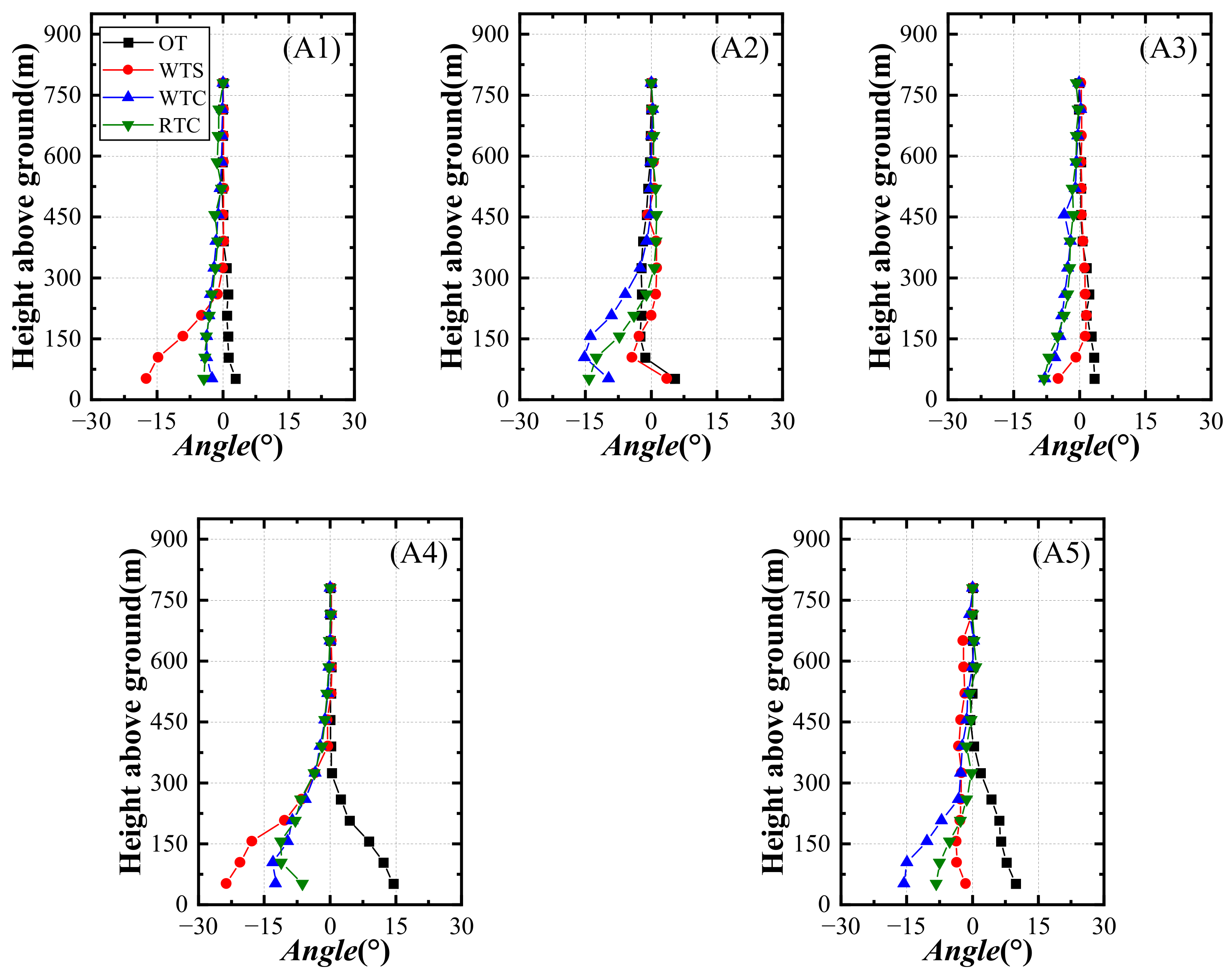
3.2. Inclination Angle

The inclination angle means the vertical flow velocity is normalized by the horizontal velocity, which is the most intractable issue in the application of the transition section. Because of transition sections with nearly slope geometry, flow is accelerated through the transition section. This could not be avoided due to the altitude difference between the model edge and the wind tunnel floor, whichever type of transition curve was used. Additionally, this issue can only be minimized by keeping the distance between measurement locations and the model edge long enough to reduce the adverse impact of the transition section.

Figure 6 shows profiles of the inclination angle at the measurement locations. The profiles are distinctly different from OT at almost every location, particularly in the region near the ground. For location A1 in the windward region, the inclination angle profiles corresponding to the terrain model with a transition section show analogous shapes to OT compared to the completely different profile in the terrain model without a transition section. The flow separation that occurred at the leading edge of the terrain model in the case of WTS greatly changed the profile and resulted in a negative value of inclination angle at the lower part.

At A2 and A3 in the leeward region, the profiles of the inclination angle in cases with transition sections are quite different from OT with a negative value. Although the profiles of WTS are not the same as those of OT, they are numerically closer, which indicates that when better velocity profile results are obtained, the additional inclination angle induced by the transition section cannot be ignored.

In the valley region, there are two measurement locations: A4 and A5. Due to the influence of flow separation in the previous analysis of mean velocity, the profiles are almost unchanged in different cases. However, it is entirely diverse in profiles of inclination angle. The inclination angle profiles in the cases of WTS, WTC, and RTC are almost opposite that of OT at heights below approximately 450 m for locations A4 and A5. Positive values have been observed in the region near the ground in the case of OT, while negative values have been found in the other cases. As shown in Figure 6, there is only a single peak ahead of locations A4 and A5. According to previous studies, flow separation off a peak or the edge of a bluff body creates a detached shear layer whose character depends strongly on the separation location [36]. For the single peak topography, separation occurs over crests and on the windward face, while the upwind topography of multiple peaks may advance the separation location. Thus, when the terrain model has been truncated, the single peak topography may be changed to multiple peaks by “artificial cliff”, and locations of the valley region show opposite inclination angles with OT. For this reason, the values of the inclination angle at locations A4 and A5 become negative in the cases with the truncated terrain model. Additionally, the differences in the cases of WTS, WTC, and RTC indicate that the separation location is determined not only by the slope of the peak but also by its geometry.

Profiles of inclination angle show more sensitivity to upwind topography than mean velocity. Although the same results of mean velocity were obtained, the opposing results were observed in inclination angle such as at locations A4 and A5. Implementing transition sections in the simulation reduces the adverse effect of flow separation at the leading edge of the terrain model to a certain extent, but there is still a discrepancy compared with the original terrain.

4. Turbulence Characteristics

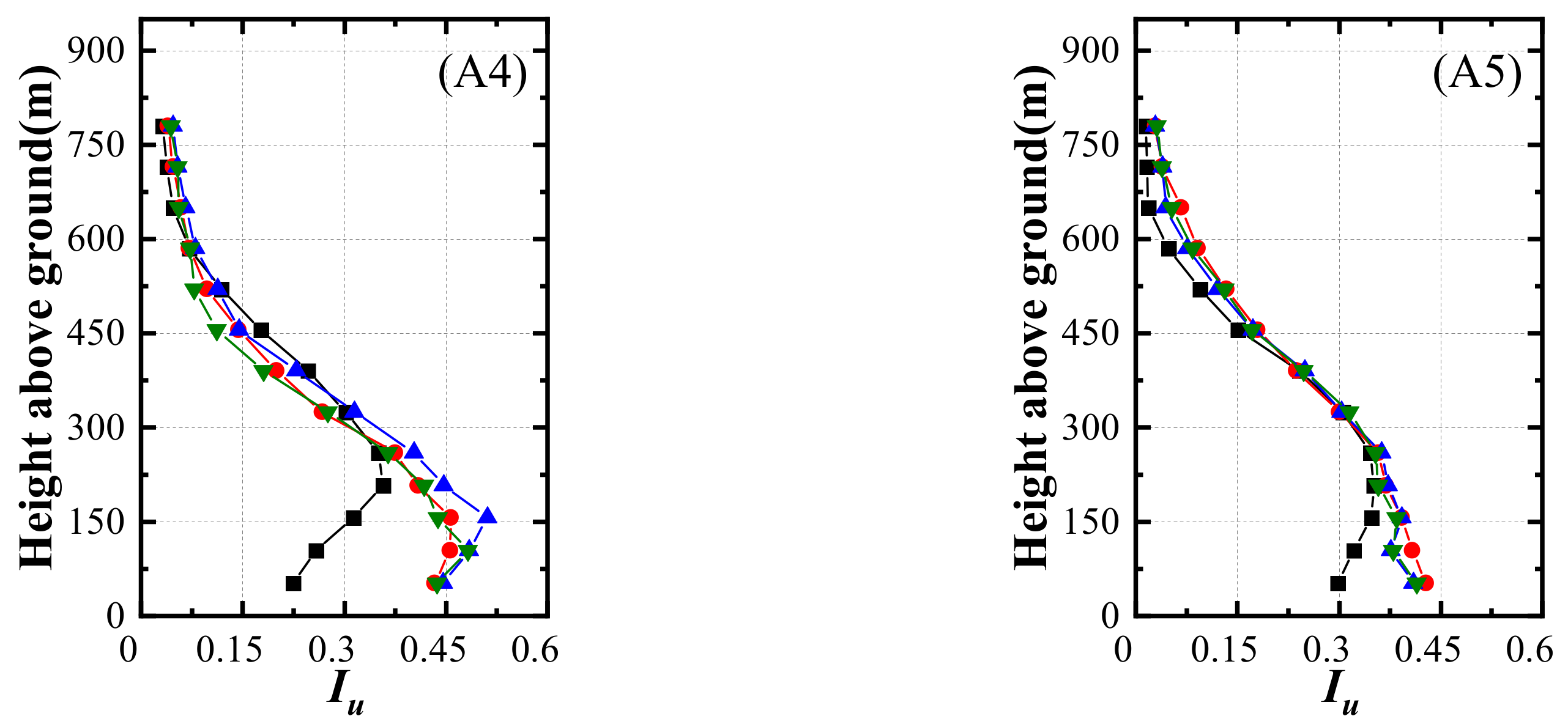
4.1. Turbulence Intensity

Turbulence intensity is given by the standard deviation of streamwise wind velocity normalized by mean velocity. The turbulence intensity profiles of the measurement locations, shown in Figure 7, intensely change in the region near the ground. Location A1 in the windward region shows higher turbulence intensities at the lower part of the profile for WTS, which indicates that flow separation induced by topographic truncation enhanced turbulence production in the region near the model edge to a greater extent, leading to inaccurate experimental results. Combined with the analysis of the mean velocity in Section 3.1, the study noted that flow separation in the case of WTS generated a similar profile in mean velocity but a different profile in turbulence intensity with OT. This means that flow separation induced by terrain truncation at the region near the terrain model edge is a difficult issue in turbulence simulation. Moreover, the lower level of turbulence intensity in cases with transition sections indicates that implementing transition sections in the experiment can effectively avoid flow separation, but there is no avoidance of the speed-up effects.

In the leeward region, for locations A2 and A3, there is at least one case with transition sections consistent with OT. Compared to WTS with lower turbulence intensity, both WTC and RTC obtained similar results with OT at location A2. As the cutting plane of location A2 is shown in Figure 5, the artificial cliff of WTS induced upwind flow separation, which was surmounted in the WTC and RTC cases. For location A3, RTC is the only case that obtained results approaching OT, which may be attributed to the fact that the ramp transition section took the place of the mountain peak in the front with producing flow separation. Coincidentally, Mcauliffe and Larose [26] used ramps to generate flow separation instead of the original topography with a mountain peak, and they also obtained acceptable results.

For the valley region, although the mean velocity profiles of the two measurement locations showed similar trends, the turbulence profiles were quite different at the elevations in the lowest 300 m above the ground. Compared with the case of OT, the other three show higher turbulence levels with decreasing height, and the largest discrepancy is found at the lower height, which is almost twice that of the OT. It seems that the increase in turbulence level caused by topographic truncation is inevitable regardless of implementation with transition sections when measurement locations are in the valley region.

4.2. Velocity Spectra

The spectra of streamwise velocity, normalized by nS_u(n)/σ², where S_u is the streamwise velocity spectra, n is the frequency, and σ is the standard deviation of velocity, are shown in Figure 8. The abscissa axis is the normalized frequency, expressed as f = nZ/U(Z), where Z is the height above ground and U(Z) is the mean velocity at height Z. The height of the spectrum shown in Figure 9 is 104 m, which is the hub height of most wind turbines.

At location A1 in the windward region, the spectra of cases with transition sections are higher than those of the WTS case, which may be attributed to flow separation suppression at the leading edge of the terrain model. Thus, large-scale vortices representing the energy of the low-frequency range are preserved. As shown in Figure 5, the side mountain range at the front of location A1 in the case of OT generated flow separation and broke up large-scale eddies into small-scale eddies, leading to lower spectra in the low-frequency range, similar to the case of WTS.

For the leeward region, spectra of four cases show little differences at location A2, but at location A3, the spectra of OT are lower than the other three in the low-frequency range. Despite the similarity in profiles of mean velocity and turbulence intensity obtained between OT and RTC, the discrepancy remains, owing to the truncation of the mountain peak ahead of location A3 in the RTC case.

According to spectra of measurement locations in the valley region, one of the distinct differences is the shift of the spectra peak toward the high-frequency range and a reduction in the low-frequency range in all cases. Strong flow separation in the valley region may account for this difference, and another peak at high-frequency might support this explanation, which is associated with a vortex-shedding process that was also measured in the wake region of an escarpment by Alvaro et al. [37]. In the case of OT, owing to the strong perturbation from complete terrain, spectra at high frequency are higher than those in the other three cases.

As indicated in Figure 8, the inertial subrange of all cases corresponds roughly with the asymptotic relation of the −2/3 slope derived by Kaimal et al. [38] in windward and leeward regions, while the slopes of spectra for measurement locations in the valley region are mismatched with less negative values, which is more significant in the case of OT. This is similar to the research of Mcauliffe and Larose [26] in which the slope of spectra is less negative in the flow separation region. In addition, experiments with the truncated terrain model may underestimate spectra in the high-frequency range due to the incompleteness of topography ahead, and the slope of spectra is also dramatically influenced with a less negative value.

5. Quantitative Analyses on Effect of Topographic Truncation

5.1. Metrics on Profiles Differences

Based on the previous analysis, topographic truncation had significant effects on mean wind characteristics and turbulence characteristics when simulating flow over an island in the wind tunnel. Hence, to quantify the differences in mean velocity, inclination angle, and turbulence intensity, the special indicators proposed by Huang et al. [17] were used, which are defined as:

$$U_x={\displaystyle \sum _{i=1}^N\frac{\left|U_i-U_{i,OT}\right|}{U_{i,OT}}}\cdot \frac{\Delta h_i}{H_w}$$

(2)

$$A_x={\displaystyle \sum _{i=1}^N\frac{\left|A_i-A_{i,OT}\right|}{\left|A_{i,OT}\right|}}\cdot \frac{\Delta h_i}{H_w}$$

(3)

$$I_x={\displaystyle \sum _{i=1}^N\frac{\left|I_i-I_{i,OT}\right|}{I_{i,OT}}}\cdot \frac{\Delta h_i}{H_w}$$

(4)

where N is the total number of measurement points along height at each measurement location, U_i is the normalized streamwise mean velocity at i-th point above the ground, U_i,OT is the normalized mean velocity at i-th point above the ground in the case of OT, Δh_i is the height difference between i-th point and (i-1)-th point, H_w is the total height at the measurement location, A_i is the inclination angle at i-th point above the ground, A_i,OT is the inclination angle at i-th point above the ground in the case of OT, I_i is the turbulence intensity at i-th point above the ground, and I_i,OT is the turbulence intensity at i-th point above the ground in the case of OT. It should be noted that in contrast to previous work [17], the absolute value is applied to Equations (2), (3), and (4) to quantify the overall differences. We also define a mean indicator (MI) to evaluate the topographic truncation effect in different cases, which can be calculated as:

$$MI={\displaystyle \sum _{j=1}^M{a}_x}\cdot \frac{1}{M}$$

(5)

where M is the total number of measurement locations and a_x means special indicators: U_x, A_x, and I_x.

Special indicators of the mean velocity, inclination angle, and turbulence intensity at each measurement location are plotted in Figure 9. The special indicator of the inclination angle shows the largest magnitude compared with the other two, while the special indicators of the mean velocity and turbulence intensity show similar magnitudes. This supports the fact that the inclination angle is likely the characteristic most influenced by topographic truncation. Hence, structures sensitive to the inclination angle should be emphasized when obtaining wind characteristics by wind tunnel simulation. As illustrated in Figure 9, the MIs of the cases with transition sections are much lower than that of the WTC in terms of the mean velocity and inclination angle. However, in terms of the inclination angle, the MIs of the cases with transition sections are slightly higher than that of the WTC. From the point of view of mean velocity and turbulence intensity, installing the transition section at the edge of the terrain model can improve the accuracy of a simulation to some extent, but only to a very limited extent. In contrast, installing transition sections at the edges of the terrain model could not improve the accuracy of the inclination angle in the wind tunnel simulation but brought additional errors in the simulation.

5.2. Metrics on Spectra Shifts

To quantify the shift of energy for spectra in frequency, three normalized frequencies [37]: f_l, f_m, and f_u, which are the cut-off frequencies of the different energy intervals, can be calculated from Equations (6) and (7):

$${\displaystyle {\int }_0^{n_c}n{s}_u(n)}/{\sigma }^{2}d[\ln (n)]-a_c=0$$

(6)

$$f_c=n_{c}Z/U(Z)$$

(7)

where n is the frequency, nS_u(n)/σ² is nonnegative and integrates to one in (−∞, +∞), and c = l, m, u. The value of a_c varies with c, and a_l = 0.05, a_m = 0.5, and a_u = 0.95. Hence, the bandwidth between f_l and f_u, which means 90% energy interval bandwidth, is calculated from Equation (8):

$$\Delta f={\log }_{10}(f_u/f_l)$$

(8)

As illustrated in Figure 10, f_m,OT and Δf_OT mean median of normalized frequency and bandwidth of normalized frequency in the case of OT, respectively. As seen in Figure 10a, the normalized median of all cases and measurement locations shows values lower than 1. This indicates that the spectra obtained from the truncation terrain model show a higher value than that from OT, which also supports our analysis in Sect. 4.2. In addition, it can be concluded that energy shifts to a low-frequency range when using the truncation terrain model to obtain spectra.

As displayed in Figure 10b, a decrease in this bandwidth is found at the measurement locations of the leeward region (A2 and A3) where the normalized bandwidth is lower than 1. However, the trend of the measurement locations at the valley region (A4 and A5) is markedly different with normalized bandwidth higher than 1. In addition, the situation for the measurement location at the windward region (A1) can be divided into two parts according to whether the transition section is applied. The value of the normalized frequency bandwidth in the case with transition section is higher than 1, while the value is lower than 1 in the case of WTS. This shows that topographic truncation brought inaccuracy into spectral bandwidth, but its effect is not certain and seems to be related to the character of the terrain where the measurement is located. Additionally, implementing transition sections at the edge of the terrain model greatly influenced the normalized frequency bandwidth, which may be attributed to the change in topography ahead leading to different flow behaviors.

6. Conclusions

A wind tunnel test for simulating flow over complex terrain was conducted in the wind tunnel laboratory of Central South University to investigate the effect of topographic truncation on wind characteristics. The analysis was carried out in two perspectives: mean wind characteristics, including mean velocity and inclination angle, and turbulence characteristics, including turbulence intensity and velocity spectra, which are fundamental parameters for flow characteristic description and are also essential for engineering applications. From the wind tunnel test, conclusions can be summarized as follows:

(1)

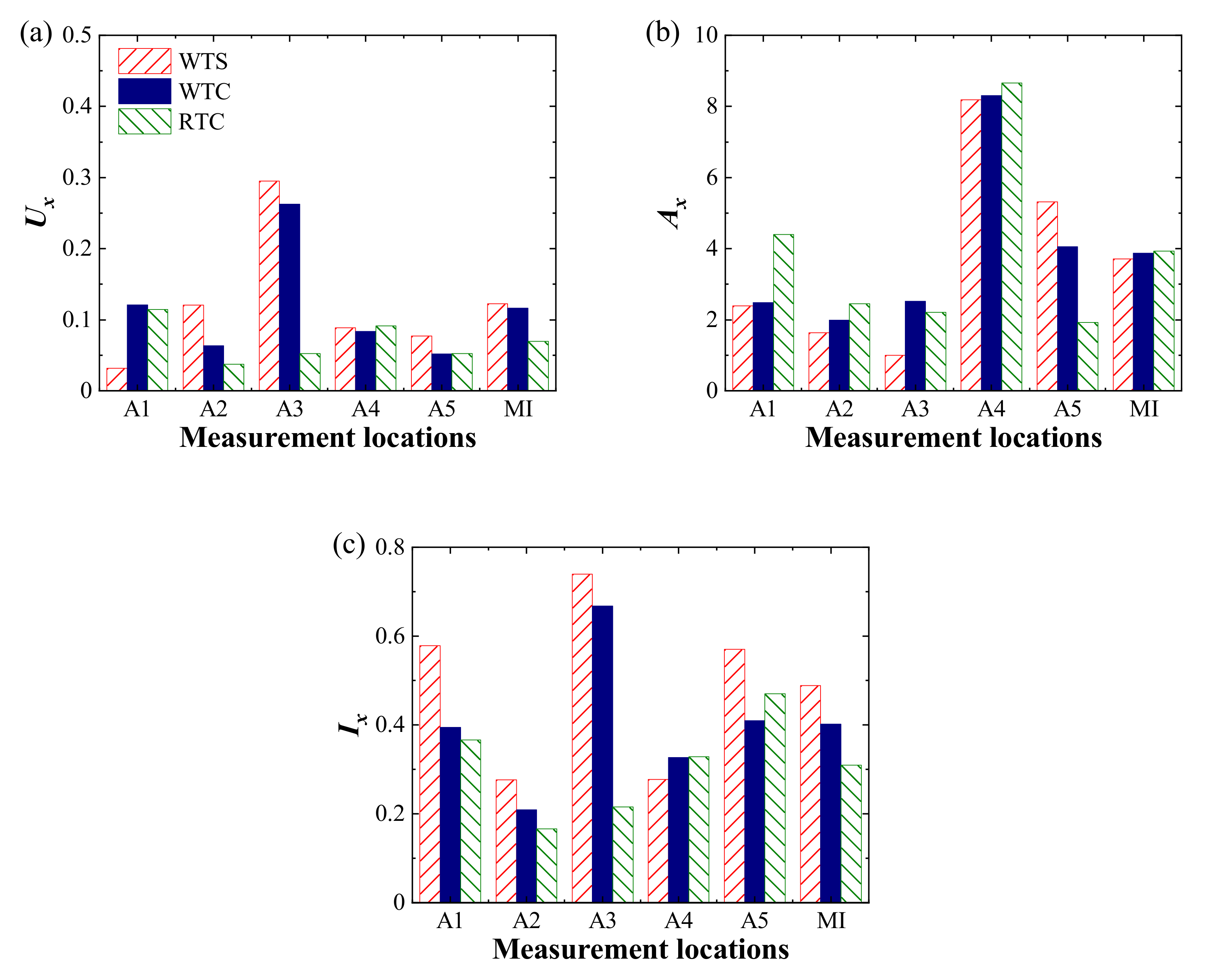
Experimental results show that the effect of topographic truncation on profiles of mean velocity and turbulence intensity is different for different regions. A greater impact of the truncation was found in windward and leeward regions. The truncation of the terrain leads to a change in topographic features, causing a change in flow behavior upwind, and is the main reason for this difference. Accurate simulation of flow behavior upwind is crucial for repeating mean velocity and turbulence intensity profiles at target locations.

(2)

By comparing the mean velocity and turbulence intensity, profiles of the inclination angle are more sensitive to topographic changes upstream, or they are more sensitive to changes in upstream flow behavior.

(3)

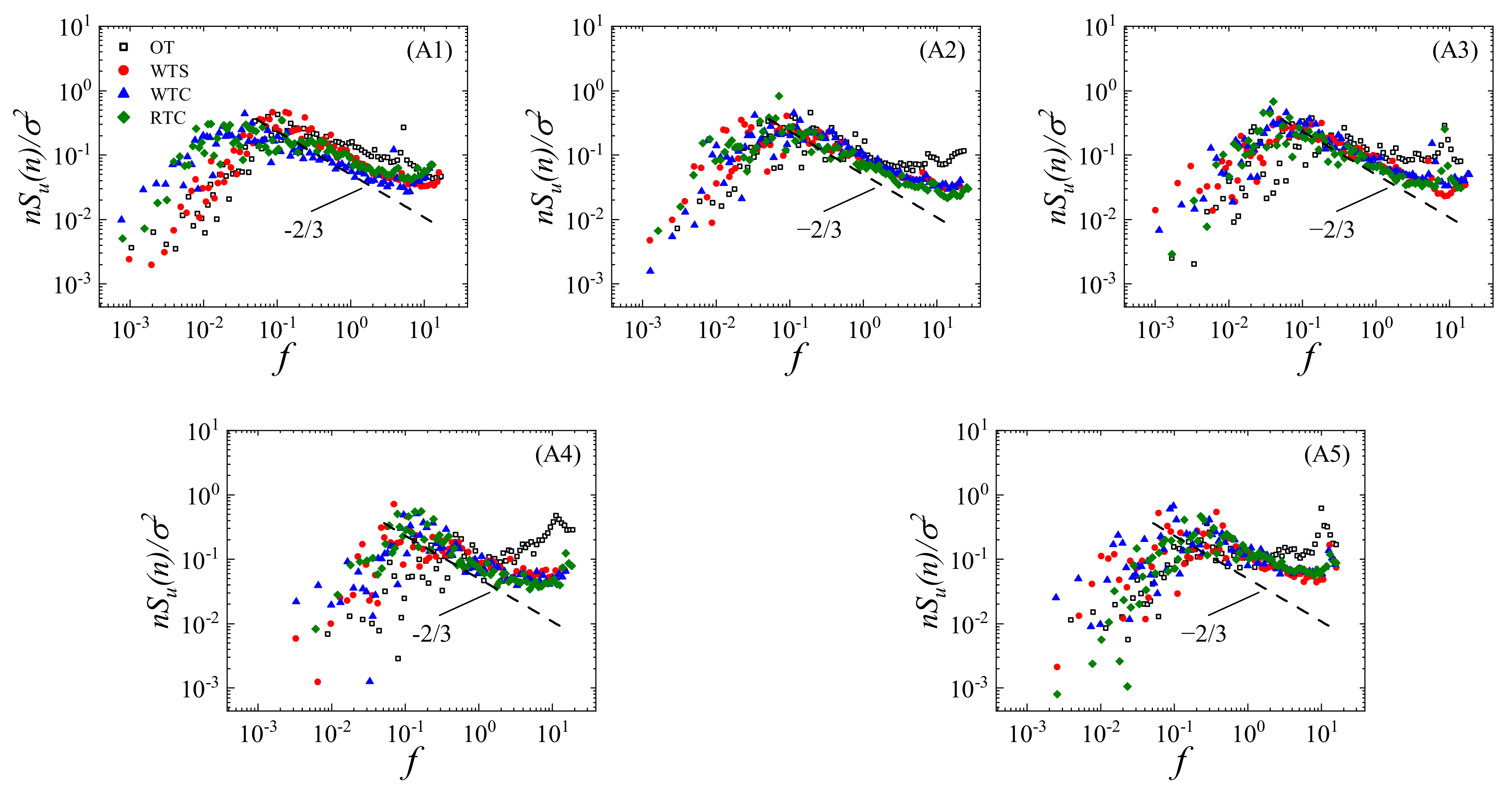
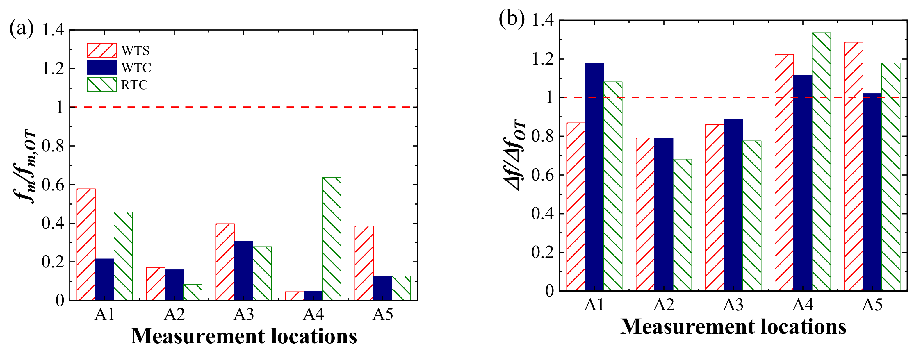
Overestimation of streamwise velocity spectra was found in cases with the truncated terrain model in the low-frequency range but underestimated in the high-frequency range. Meanwhile, the slope of the spectra is influenced by a less negative value at the inertial subrange. Moreover, the normalized bandwidth representing the 90% energy interval is influenced by the topographic truncation, but the effect relates to the measurement locations. The bandwidth of windward and leeward regions narrows down, while the bandwidth of the valley region broadens.

(4)

Transition sections used in this study have only limited effectiveness. Transition sections can only curb flow separation at the edge of the terrain model, but the change in flow behavior caused by the absence of topographic features due to topographic truncation cannot be resolved. In addition, the implementation of transition sections at the model edge may introduce additional errors into the experiment.

References

1. Kilpatrick, R.J.; Hangan, H.; Siddiqui, K.; Lange, J.; Mann, J. Turbulent Flow Characterization Near the Edge of a Steep Escarpment. J. Wind Eng. Ind. Aerodyn. 2021, 212, 104605. [Google Scholar] [CrossRef]
2. Ren, H.; Wu, Y. Turbulent Boundary Layers Over Smooth and Rough Forward-facing Steps. Phys. Fluids 2011, 23, 45102. [Google Scholar] [CrossRef]
3. Wu, Y.; Ren, H. On the Impacts of Coarse-scale Models of Realistic Roughness on a Forward-facing Step Turbulent Flow. Int. J. Heat Fluid Flow 2013, 40, 15–31. [Google Scholar] [CrossRef]
4. Conan, B.; van Beeck, J.; Aubrun, S. Sand Erosion Technique Applied to Wind Resource Assessment. J. Wind Eng. Ind. Aerodyn. 2012, 104, 322–329. [Google Scholar] [CrossRef]
5. Jiao, A.; Shen, Y.; Wang, Z.; Chen, T.; Tao, H.; Xu, Z.; Fan, C. Experimental Study on the Effect of Canyon Cross Wind Yaw Angle on Airflow and Flame Characteristics in a Tunnel. J. Wind Eng. Ind. Aerodyn. 2021, 213, 104616. [Google Scholar] [CrossRef]
6. Nanos, E.M.; Yilmazlar, K.; Zanotti, A.; Croce, A.; Bottasso, C.L. Wind Tunnel Testing of a Wind Turbine in Complex Terrain. J. Phys. Conf. Ser. 2020, 1618, 032041. [Google Scholar] [CrossRef]
7. Ayotte, K.W.; Hughes, D.E. Observations of Boundary-layer Wind-tunnel Flow Over Isolated Ridges of Varying Steepness and Roughness. Bound.-Layer Meteorol. 2004, 112, 525–556. [Google Scholar] [CrossRef]
8. Kilpatrick, R.; Hangan, H.; Siddiqui, K.; Parvu, D.; Lange, J.; Mann, J.; Berg, J. Effect of Reynolds Number and Inflow Parameters on Mean and Turbulent Flow Over Complex Topography. Wind Energ. Sci. 2016, 1, 237–254. [Google Scholar] [CrossRef] [Green Version]
9. Berg, J.; Mann, J.; Bechmann, A.; Courtney, M.S.; Jørgensen, H.E. The Bolund Experiment, Part I: Flow Over a Steep, Three-dimensional Hill. Bound.-Layer Meteorol. 2011, 141, 219. [Google Scholar] [CrossRef] [Green Version]
10. Lange, J.; Mann, J.; Berg, J.; Parvu, D.; Kilpatrick, R.; Costache, A.; Jubayer, C.; Siddiqui, K.; Hangan, H. For Wind Turbines in Complex Terrain, the Devil Is in the Detail. Environ. Res. Lett. 2017, 12, 94020. [Google Scholar] [CrossRef]
11. Yeow, T.; Cuerva-tejero, A.; Perez-alvarez, J. Reproducing the Bolund Experiment in Wind Tunnel. Wind Energy 2015, 18, 153–169. [Google Scholar] [CrossRef] [Green Version]
12. Lange, J.; Mann, J.; Angelou, N.; Berg, J.; Sjöholm, M.; Mikkelsen, T. Variations of the Wake Height Over the Bolund Escarpment Measured by a Scanning Lidar. Bound.-Layer Meteorol. 2016, 159, 147–159. [Google Scholar] [CrossRef] [Green Version]
13. Liao, H.; Jing, H.; Ma, C.; Tao, Q.; Li, Z. Field Measurement Study on Turbulence Field by Wind Tower and Windcube Lidar in Mountain Valley. J. Wind Eng. Ind. Aerodyn. 2020, 197, 104090. [Google Scholar] [CrossRef]
14. Jing, H.; Liao, H.; Ma, C.; Tao, Q.; Jiang, J. Field Measurement Study of Wind Characteristics at Different Measuring Positions in a Mountainous Valley. Exp. Therm. Fluid Sci. 2020, 112, 109991. [Google Scholar] [CrossRef]
15. Taylor, P.A.; Teunissen, H.W. The Askervein Hill Project: Overview and Background Data. Bound.-Layer Meteorol. 1987, 39, 15–39. [Google Scholar] [CrossRef]
16. Salmon, J.R.; Teunissen, H.W.; Mickle, R.E.; Taylor, P.A. The Kettles Hill Project: Field Observations, Wind-tunnel Simulations and Numerical Model Predictions for Flow Over a Low Hill. Bound.-Layer Meteorol. 1988, 43, 309–343. [Google Scholar] [CrossRef]
17. Huang, G.; Cheng, X.; Peng, L.; Li, M. Aerodynamic Shape of Transition Curve for Truncated Mountainous Terrain Model in Wind Field Simulation. J. Wind Eng. Ind. Aerodyn. 2018, 178, 80–90. [Google Scholar] [CrossRef]
18. Han, Y.; Shen, L.; Xu, G.; Cai, C.S.; Zhang, J. Multiscale Simulation of Wind Field on a Long Span Bridge Site in Mountainous Area. J. Wind Eng. Ind. Aerodyn. 2018, 177, 260–274. [Google Scholar] [CrossRef]
19. Zhang, M.; Zhang, J.; Li, Y.; Yu, J.; Wu, L. Wind Characteristics in the High-altitude Difference at Bridge Site by Wind Tunnel Tests. Wind Struct. 2020, 30, 548–557. [Google Scholar]
20. Zhang, M.; Yu, J.; Zhang, J.; Wu, L.; Li, Y. Study on the Wind-field Characteristics Over a Bridge Site Due to the Shielding Effects of Mountains in a Deep Gorge Via Numerical Simulation. Adv. Struct. Eng. 2019, 22, 3055–3065. [Google Scholar]
21. Jubayer, C.M.; Hangan, H. A Hybrid Approach for Evaluating Wind Flow Over a Complex Terrain. J. Wind Eng. Ind. Aerodyn. 2018, 175, 65–76. [Google Scholar] [CrossRef]
22. Maurizi, A.; Palma, J.; Castro, F.A. Numerical Simulation of the Atmospheric Flow in a Mountainous Region of the North of Portugal. J. Wind Eng. Ind. Aerodyn. 1998, 74–76, 219–228. [Google Scholar] [CrossRef]
23. Hu, P.; Li, Y.; Huang, G.; Kang, R.; Liao, H. The Appropriate Shape of the Boundary Transition Section for a Mountain-gorge Terrain Model in a Wind Tunnel Test. Wind Struct. 2015, 20, 15–36. [Google Scholar] [CrossRef]
24. Hu, P.; Han, Y.; Xu, G.; Li, Y.; Xue, F. Numerical Simulation of Wind Fields at the Bridge Site in Mountain-gorge Terrain Considering an Updated Curved Boundary Transition Section. J. Aerosp. Eng. 2018, 31, 4018008. [Google Scholar] [CrossRef]
25. Chen, X.; Liu, Z.; Wang, X.; Chen, Z.; Xiao, H.; Zhou, J. Experimental and Numerical Investigation of Wind Characteristics Over Mountainous Valley Bridge Site Considering Improved Boundary Transition Sections. Appl. Sci. 2020, 10, 751. [Google Scholar] [CrossRef] [Green Version]
26. Mcauliffe, B.R.; Larose, G.L. Reynolds-number and Surface-modeling Sensitivities for Experimental Simulation of Flow Over Complex Topography. J. Wind Eng. Ind. Aerodyn. 2012, 104–106, 603–613. [Google Scholar] [CrossRef]
27. Røkenes, K.; Krogstad, P. Wind Tunnel Simulation of Terrain Effects on Wind Farm Siting. Wind Energy 2009, 12, 391–410. [Google Scholar] [CrossRef]
28. Gao, D.L.; Deng, Z.; Yang, W.H.; Chen, W.L. Review of the excitation mechanism and aerodynamic flow control of vortex-induced vibration of the main girder for long-span bridges: A vortex-dynamics approach. J. Fluids Struct. 2021, 105, 103348. [Google Scholar] [CrossRef]
29. Chen, W.L.; Zhang, Q.Q.; Li, H.; Hu, H. An experimental investigation on vortex induced vibration of a flexible inclined cable under a shear flow. J. Fluids Struct. 2015, 54, 297–311. [Google Scholar] [CrossRef]
30. Li, H.; Chen, W.L.; Xu, F.; Li, F.C.; Ou, J.P. A numerical and experimental hybrid approach for the investigation of aerodynamic forces on stay cables suffering from rain-wind induced vibration. J. Fluids Struct. 2010, 26, 1195–1215. [Google Scholar] [CrossRef]
31. He, X.H.; Zuo, T.H.; Zou, Y.F.; Yan, L.; Tang, L.B. Experimental study on aerodynamic characteristics of a high-speed train on viaducts in turbulent crosswinds. J. Cent. South Univ. 2020, 27, 2465–2478. [Google Scholar] [CrossRef]
32. Bowen, A. Modelling of Strong Wind Flows Over Complex Terrain at Small Geometric Scales. J. Wind Eng. Ind. Aerodyn. 2003, 91, 1859–1871. [Google Scholar] [CrossRef]
33. Holmes, J.D. Wind Loading of Structures, 3rd ed.; CRC Press: Los Angeles, CA, USA, 2015; pp. 187–188. [Google Scholar]
34. Cermak, J.E. Physical Modelling of Flow and Dispersion Over Complex Terrain. In Boundary Layer Structure, 1st ed.; Hadassah, K., Nathan, D., Eds.; Springer: Dordrecht, The Netherlands, 1984; pp. 261–292. [Google Scholar]
35. Conan, B. Wind Resource Assessment in Complex Terrain by Wind Tunnel Modelling. Ph.D. Thesis, Orléans University, Orléans, France, 2012. [Google Scholar]
36. Derickson, R.; Peterka, J. Development of a Powerful Hybrid Tool for Evaluating Wind Power in Complex Terrain: Atmospheric Numerical Models and Wind Tunnels. In Proceedings of the 23rd Asme Wind Energy Symposium: American Institute of Aeronautics and Astronautics, Reno, NV, USA, 5–8 January 2004. [Google Scholar]
37. Cuerva-tejero, A.; Avila-sanchez, S.; Gallego-castillo, C.; Lopez-garcia, O.; Perez-alvarez, J.; Yeow, T.S. Measurement of spectra over the Bolund hill in wind tunnel. Wind Energy 2018, 21, 87–99. [Google Scholar] [CrossRef]
38. Kaimal, J.C.; Wyngaard, J.C.; Izumi, Y.; Coté, O.R. Spectral characteristics of surface-layer turbulence. Q. J. R. Meteorol. Soc. 1972, 98, 563–589. [Google Scholar] [CrossRef]
Figure 1. Topography of island and measurement locations.
Applsci 12 02477 g001
Figure 2. Transition section: (a) sketch of transition section; (b) sketch of transition curve.
Applsci 12 02477 g002
Figure 3. The test model at wind tunnel: (a) OT; (b) WTS; (c) WTC; (d) RTC.
Applsci 12 02477 g003
Figure 4. Profiles of mean velocity at measurement locations: (A1) location A1; (A2) location A2; (A3) location A3; (A4) location A4; (A5) location A5.
Applsci 12 02477 g004
Figure 5. East-West cutting planes of measurement locations: (A1) location A1; (A2) location A2; (A3) location A3; (A4) location A4; (A5) location A5.
Applsci 12 02477 g005
Figure 6. Profiles of inclination angle at measurement locations: (A1) location A1; (A2) location A2; (A3) location A3; (A4) location A4; (A5) location A5.
Applsci 12 02477 g006
Figure 7. Profiles of turbulence intensity at measurement locations: (A1) location A1; (A2) location A2; (A3) location A3; (A4) location A4; (A5) location A5.
Applsci 12 02477 g007aApplsci 12 02477 g007b
Figure 8. Normalized streamwise spectra for measurement locations at a height of 104 m: (A1) location A1; (A2) location A2; (A3) location A3; (A4) location A4; (A5) location A5.
Applsci 12 02477 g008
Figure 9. Special indexes at measurement locations: (a) mean velocity; (b) inclination angle; (c) turbulence intensity.
Applsci 12 02477 g009
Figure 10. Metrics on spectra shifts at measurement locations: (a) median of the normalized frequency; (b) the bandwidth of the normalized frequency.
Applsci 12 02477 g010
Publisher’s Note: MDPI stays neutral with regard to jurisdictional claims in published maps and institutional affiliations.