
Estimation System of Disturbance Force and Torque for Underwater Robot Based on Artificial Lateral Line


Abstract
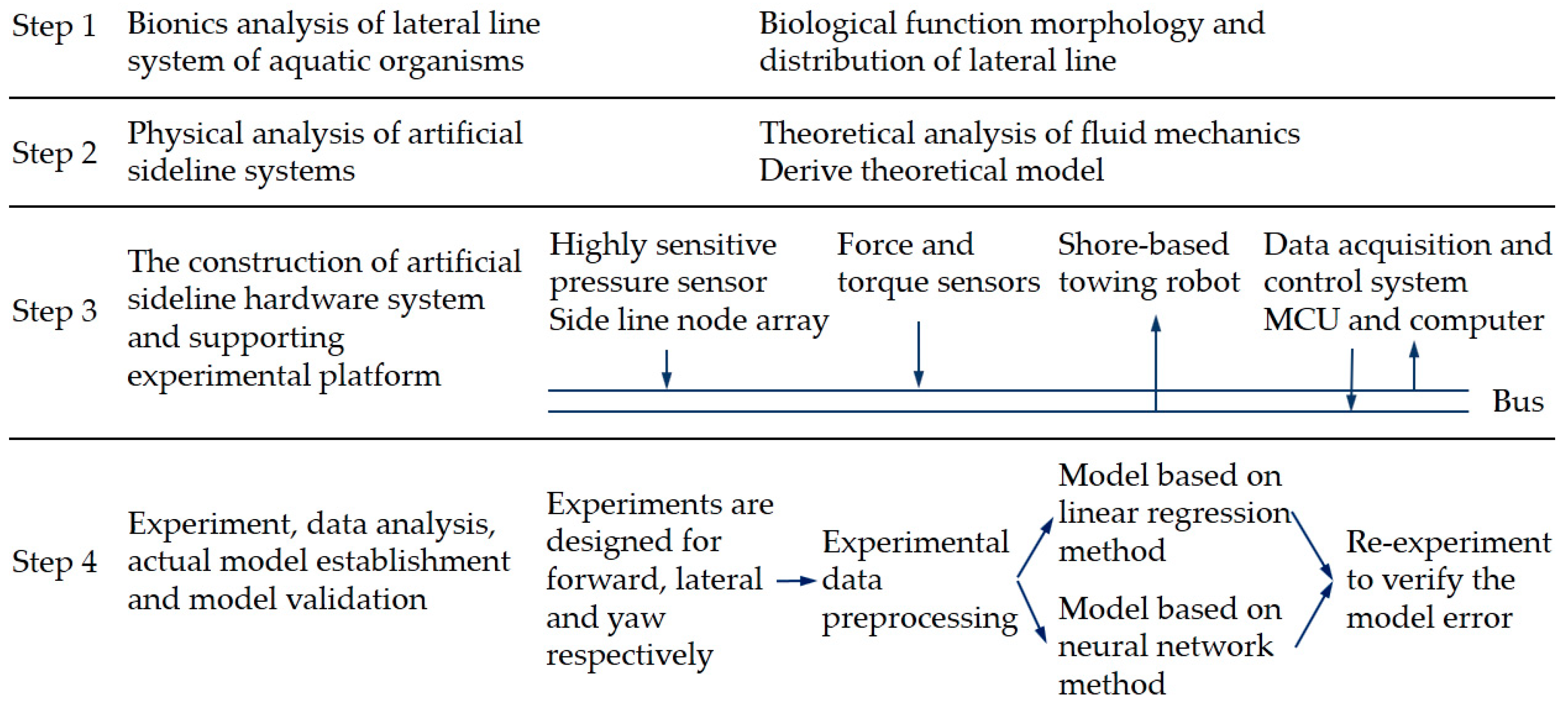
:1. Introduction
2. Lateral-Line System and Artificial Lateral-Line System
2.1. Lateral Lines of Aquatic Organisms
2.2. Physical Device of Artificial Lateral-Line System Suitable for the Underwater Robot
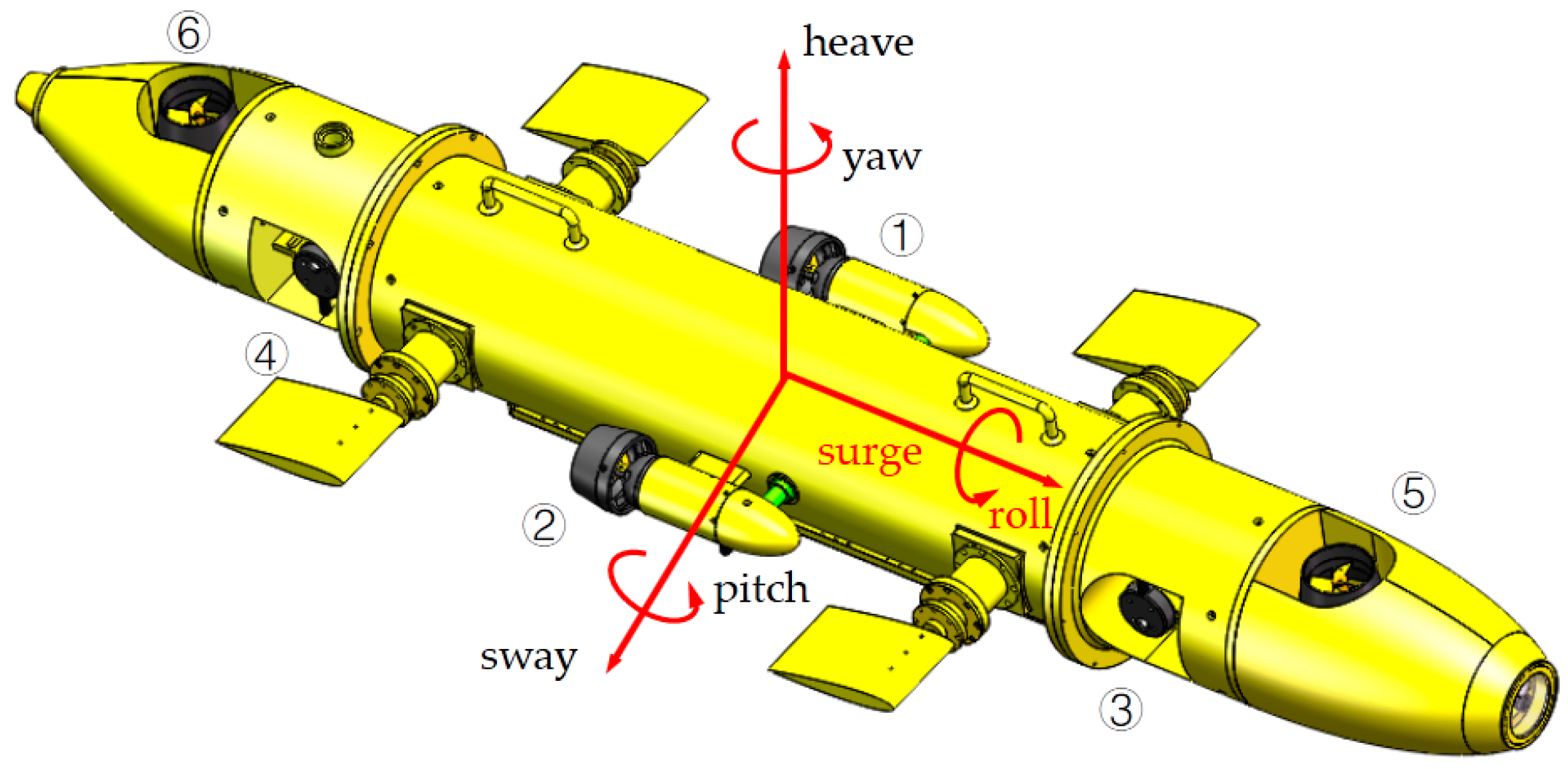
2.2.1. Introduction of Underwater Robot System
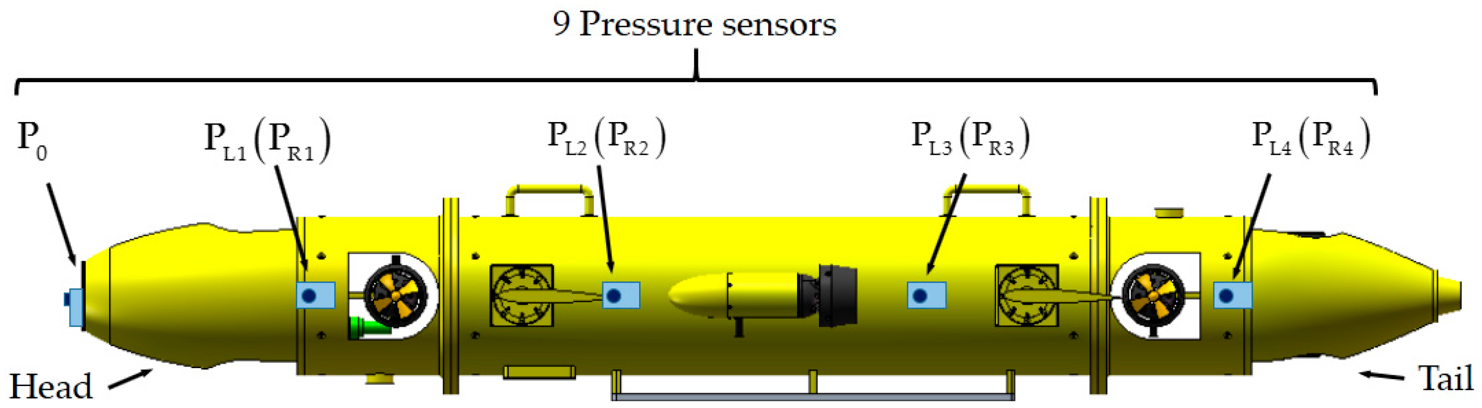
2.2.2. Introduction of the Artificial Lateral-Line System of Underwater Robot
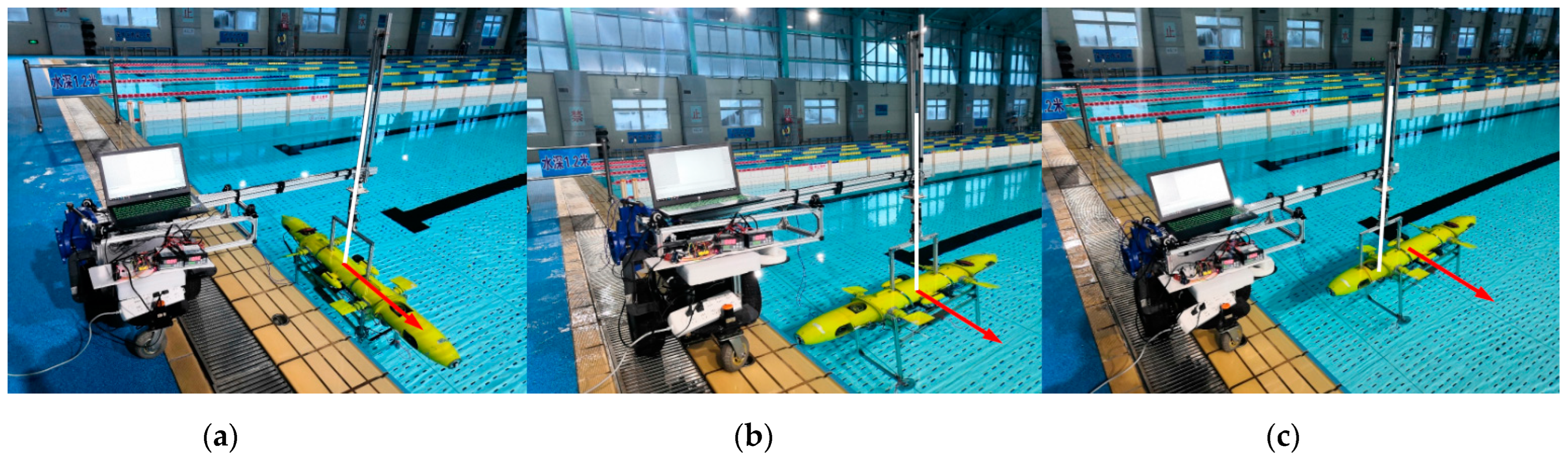
2.3. Experimental Platform for Artificial Lateral-Line System of Underwater Robot
3. Methods of Artificial Lateral-Line System for the Underwater Robot
3.1. Relationship between Disturbance Force and Lateral-Line-System Data on Surge
3.2. Relationship between Disturbance Force and Lateral-Line-System Data on Sway
3.3. Relationship between Disturbance Torque and Lateral-Line-System Data on Yaw
4. Experiment and Data Preprocessing of Artificial Lateral-Line System
4.1. Experiment of Artificial Lateral-Line System for the Underwater Robot
4.2. Experimental Results and Data Preprocessing
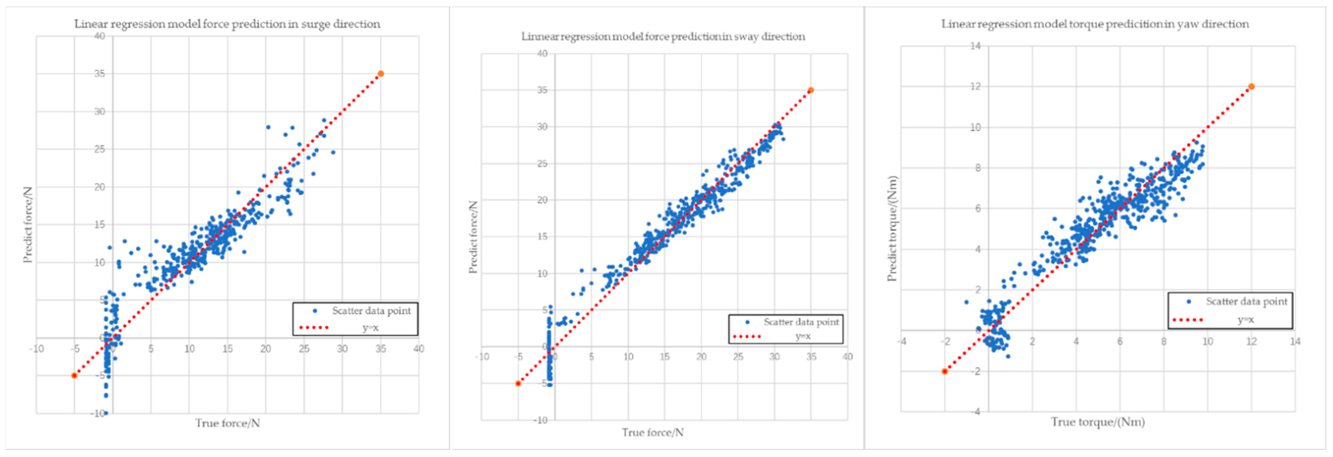
5. Experimental Data Analysis Based on Linear Regression
5.1. Data Analysis of Disturbance Force and Lateral-Line System Data on Surge
5.2. Data Analysis of Disturbance Force and Lateral-Line-System Data on Sway
5.3. Data Analysis of Disturbance Force and Lateral-Line-System Data on Yaw
5.4. Error Analysis of Linear Regression
6. Experimental Data Analysis Based on Artificial Neural Network
7. Conclusions
Author Contributions
Funding
Institutional Review Board Statement
Informed Consent Statement
Data Availability Statement
Acknowledgments
Conflicts of Interest
References
- FreiwAld, A.; Beuck, L.; Rüggeberg, A.; Taviani, M.; Hebbeln, D. The white coral community in the central Mediterranean Sea revealed by ROV surveys. Oceanography 2009, 22, 58–74. [Google Scholar] [CrossRef] [Green Version]
- Li, J.; Zhou, H.; Huang, H.; Yang, X.; Wan, Z.; Wan, L. Design and vision based autonomous capture of sea organism with absorptive type remotely operated vehicle. IEEE Access 2018, 6, 73871–73884. [Google Scholar]
- Khatib, O.; Yeh, X.; Brantner, G.; Soe, B.; Kim, B.; Ganguly, S.; Stuart, H.; Wang, S.; Cutkosky, M.; Edsinger, A. Ocean one: A robotic avatar for oceanic discovery. IEEE Robot. Autom. Mag. 2016, 23, 20–29. [Google Scholar] [CrossRef]
- Jiang, Y.; Ma, Z.; Zhang, D.J.B. Flow field perception based on the fish lateral line system. Bioinspiration Biomim. 2019, 14, 041001. [Google Scholar] [CrossRef]
- Shao, X.; Liu, J.; Cao, H.; Shen, C.; Wang, H. Robust dynamic surface trajectory tracking control for a quadrotor UAV via extended state observer. Int. J. Robust Nonlinear Control 2018, 28, 2700–2719. [Google Scholar] [CrossRef]
- Wu, Y.; Low, K.H.; Lv, C. Cooperative path planning for heterogeneous unmanned vehicles in a search-and-track mission aiming at an underwater target. IEEE Trans. Veh. Technol. 2020, 69, 6782–6787. [Google Scholar] [CrossRef]
- Bleckmann, H.; Zelick, R. Lateral line system of fish. Integr. Zool. 2009, 4, 13–25. [Google Scholar] [CrossRef]
- Mogdans, J.; Bleckmann, H. The mechanosensory lateral line of jawed fishes. In Sensory Biology of Jawed Fishes; New Insights Science Publishers Inc.: Enfield, NH, USA, 2001. [Google Scholar]
- Parker, G.H. The Function of the Lateral-Line Organs in Fishes; US Government Printing Office: Washington, DC, USA, 1904.
- Dijkgraaf, S. The functioning and significance of the lateral-line organs. Biol. Rev. 1963, 38, 51–105. [Google Scholar] [CrossRef]
- Lloyd, E.; Olive, C.; Stahl, B.A.; Jaggard, J.B.; Amaral, P.; Duboué, E.R.; Keene, A.C. Evolutionary shift towards lateral line dependent prey capture behavior in the blind Mexican cavefish. Dev. Biol. 2018, 441, 328–337. [Google Scholar] [CrossRef]
- Oteiza, P.; Odstrcil, I.; Lauder, G.; Portugues, R.; Engert, F. A novel mechanism for mechanosensory-based rheotaxis in larval zebrafish. Nature 2017, 547, 445–448. [Google Scholar] [CrossRef] [Green Version]
- Schwaner, M.; Hsieh, S.; Swalla, B.; McGowan, C. An Introduction to an Evolutionary Tail: EvoDevo, Structure, and Function of Post-Anal Appendages. Integr. Comp. Biol. 2021, 61, 352–357. [Google Scholar] [CrossRef] [PubMed]
- Abdulsadda, A.T.; Tan, X. An artificial lateral line system using IPMC sensor arrays. Int. J. Smart Nano Mater. 2012, 3, 226–242. [Google Scholar] [CrossRef] [Green Version]
- Shizhe, T. Underwater artificial lateral line flow sensors. Microsyst. Technol. 2014, 20, 2123–2136. [Google Scholar] [CrossRef]
- Ristroph, L.; Liao, J.C.; Zhang, J. Lateral line layout correlates with the differential hydrodynamic pressure on swimming fish. Phys. Rev. Lett. 2015, 114, 018102. [Google Scholar] [CrossRef] [PubMed] [Green Version]
- Yang, Y.; Chen, J.; Engel, J.; Pandya, S.; Chen, N.; Tucker, C.; Coombs, S.; Jones, D.L.; Liu, C. Distant touch hydrodynamic imaging with an artificial lateral line. Proc. Natl. Acad. Sci. USA 2006, 103, 18891–18895. [Google Scholar] [CrossRef] [PubMed] [Green Version]
- Bora, M.; Kottapalli, A.G.P.; Miao, J.; Triantafyllou, M.S. Sensing the flow beneath the fins. Bioinspiration Biomim. 2018, 13, 025002. [Google Scholar] [CrossRef]
- Han, Z.; Liu, L.; Wang, K.; Song, H.; Chen, D.; Wang, Z.; Niu, S.; Zhang, J.; Ren, L. Artificial hair-like sensors inspired from nature: A review. J. Bionic Eng. 2018, 15, 409–434. [Google Scholar] [CrossRef]
- Tao, J.; Yu, X.B. Hair flow sensors: From bio-inspiration to bio-mimicking—A review. Smart Mater. Struct. 2012, 21, 113001. [Google Scholar] [CrossRef]
- Chen, X.; Zhu, G.; Yang, X.; Hung, D.L.; Tan, X. Model-based estimation of flow characteristics using an ionic polymer–metal composite beam. IEEE/ASME Trans. Mechatron. 2012, 18, 932–943. [Google Scholar] [CrossRef]
- Klein, A.; Bleckmann, H. Determination of object position, vortex shedding frequency and flow velocity using artificial lateral line canals. Beilstein J. Nanotechnol. 2011, 2, 276–283. [Google Scholar] [CrossRef] [Green Version]
- Chambers, L.D.; Akanyeti, O.; Venturelli, R.; Ježov, J.; Brown, J.; Kruusmaa, M.; Fiorini, P.; Megill, W. A fish perspective: Detecting flow features while moving using an artificial lateral line in steady and unsteady flow. J. R. Soc. Interface 2014, 11, 20140467. [Google Scholar] [CrossRef] [PubMed] [Green Version]
- Venturelli, R.; Akanyeti, O.; Visentin, F.; Ježov, J.; Chambers, L.D.; Toming, G.; Brown, J.; Kruusmaa, M.; Megill, W.M.; Fiorini, P. Hydrodynamic pressure sensing with an artificial lateral line in steady and unsteady flows. Bioinspiration Biomim. 2012, 7, 036004. [Google Scholar] [CrossRef] [PubMed]
- Wang, W.; Zhang, X.; Zhao, J.; Xie, G. Sensing the neighboring robot by the artificial lateral line of a bio-inspired robotic fish. In Proceedings of the 2015 IEEE/RSJ International Conference on Intelligent Robots and Systems (IROS), Hamburg, Germany, 28 September–2 October 2015; pp. 1565–1570. [Google Scholar]
- DeVries, L.; Lagor, F.D.; Lei, H.; Tan, X.; Paley, D.A. Distributed flow estimation and closed-loop control of an underwater vehicle with a multi-modal artificial lateral line. Bioinspiration Biomim. 2015, 10, 025002. [Google Scholar] [CrossRef] [PubMed]
- Bleckmann, H. Role of the lateral line in fish behaviour. In The Behaviour of Teleost Fishes; Springer: Berlin/Heidelberg, Germany, 1986; pp. 177–202. [Google Scholar]
- Ghysen, A.; Dambly-Chaudière, C. The lateral line microcosmos. Genes Dev. 2007, 21, 2118–2130. [Google Scholar] [CrossRef] [Green Version]
- Liu, G.; Wang, A.; Wang, X.; Liu, P. A review of artificial lateral line in sensor fabrication and bionic applications for robot fish. Appl. Bionics Biomech. 2016, 2016, 4732703. [Google Scholar] [CrossRef]
- Ai, X.; Kang, S.; Chou, W. System design and experiment of the hybrid underwater vehicle. In Proceedings of the 2018 International Conference on Control and Robots (ICCR), Hong Kong, China, 15–17 September 2018; pp. 68–72. [Google Scholar]
- Kang, S.; Rong, Y.; Chou, W. Antidisturbance control for AUV trajectory tracking based on fuzzy adaptive extended state Observer. Sensors 2020, 20, 7084. [Google Scholar] [CrossRef]
- Fossen, T.I. Handbook of Marine Craft Hydrodynamics and Motion Control; John Wiley & Sons: Hoboken, NJ, USA, 2011. [Google Scholar]
- Zdravkovich, M.M. Flow around Circular Cylinders: Volume 2: Applications; Oxford University Press: Oxford, UK, 1997; Volume 2. [Google Scholar]
- Bauman, R.P.; Schwaneberg, R. Interpretation of Bernoulli’s equation. Phys. Teach. 1994, 32, 478–488. [Google Scholar] [CrossRef]
- Mello, R.G.; Oliveira, L.F.; Nadal, J. Digital Butterworth filter for subtracting noise from low magnitude surface electromyogram. Comput. Methods Programs Biomed. 2007, 87, 28–35. [Google Scholar] [CrossRef]
- Montgomery, D.C.; Peck, E.A.; Vining, G.G. Introduction to Linear Regression Analysis; John Wiley & Sons: Hoboken, NJ, USA, 2021. [Google Scholar]
- Seber, G.A.; Lee, A.J. Linear Regression Analysis; John Wiley & Sons: Hoboken, NJ, USA, 2012. [Google Scholar]
- Wang, S.-C. Artificial neural network. In Interdisciplinary Computing in Java Programming; Springer: Berlin/Heidelberg, Germany, 2003; pp. 81–100. [Google Scholar]


| Author | Achievements |
|---|---|
| Abdulsadda et al. [14] | An ALL system based on IPMC sensors was presented to localize the dipole source (vibrating sphere) underwater. |
| Ristroph et al. [16] | The locations with the largest pressure change were concentrated, and a simulation was presented to mimic the flows encountered during swimming. |
| Yang et al. [17] | An ALL system with a distributed linear array was presented, which can successfully perform dipole-source localization and hydrodynamic wake detection. |
| Chen et al. [21] | A dynamic model was developed for the IPMC beam under the flow to estimate fluid properties and flow parameters. |
| Klein et al. [22] | An ALL system equipped with optical-flow sensors was presented to detect water motions, vortices or water (air) movement. |
| Chambers et al. [23] | To detect and navigate turbulent flows and sense fluid interactions for underwater vehicles, a total of 33 pressure sensors were used under Karman vortex streets at different parameters. |
| Venturelli et al. [24] | To sense the underwater environment better, 20 pressure sensors were used to distinguish the Karman vortex streets and uniform flow. |
| Wang et al. [25] | A fish robot with ALL system was presented to detect the beating frequency of its neighboring robot and the distance between the robots. |
| DeVries et al. [26] | Theoretically justified nonlinear estimation strategies were presented to perceive the environment using 4 pressure sensors, and to use the strategies to construct a feedback-control system. |
| Direction | |||
|---|---|---|---|
| surge | |||
| sway | |||
| yaw |
| Direction | |||
|---|---|---|---|
| surge | |||
| sway | |||
| yaw |
Publisher’s Note: MDPI stays neutral with regard to jurisdictional claims in published maps and institutional affiliations. |
© 2022 by the authors. Licensee MDPI, Basel, Switzerland. This article is an open access article distributed under the terms and conditions of the Creative Commons Attribution (CC BY) license (https://creativecommons.org/licenses/by/4.0/).
Share and Cite
Kang, S.; Chou, W.; Yu, J. Estimation System of Disturbance Force and Torque for Underwater Robot Based on Artificial Lateral Line. Appl. Sci. 2022, 12, 3060. https://doi.org/10.3390/app12063060
Kang S, Chou W, Yu J. Estimation System of Disturbance Force and Torque for Underwater Robot Based on Artificial Lateral Line. Applied Sciences. 2022; 12(6):3060. https://doi.org/10.3390/app12063060
Chicago/Turabian StyleKang, Song, Wusheng Chou, and Junhao Yu. 2022. "Estimation System of Disturbance Force and Torque for Underwater Robot Based on Artificial Lateral Line" Applied Sciences 12, no. 6: 3060. https://doi.org/10.3390/app12063060
APA StyleKang, S., Chou, W., & Yu, J. (2022). Estimation System of Disturbance Force and Torque for Underwater Robot Based on Artificial Lateral Line. Applied Sciences, 12(6), 3060. https://doi.org/10.3390/app12063060