Interval Analysis of Vibro-Acoustic Systems by the Enclosing Interval Finite-Element Method

Abstract

Traditional interval analysis methods for interior vibro-acoustic system with uncertain-but-bounded parameters are based on interval perturbation theory. However, the solution sets by traditional interval finite-element methods are intrinsically not capable of reflecting the actual bounds of results, due to the non-conservative approximation for neglecting the high-order terms of both Taylor and Neumann series. In order to cope with this problem, this paper introduces the concept of unimodal components from structural mechanics to factorize the uncertainties, and a new enclosing interval-finite element method (enclosing-IFEM) is proposed to predict the uncertain vibro-acoustic response. In the enclosing-IFEM, the global matrix is assembled with the mixed-nodal-element strategy (MNE), which is different from the element-by-element assembly strategy. Thus, the vibro-acoustic coupling equation can be transformed into an iterative enclosure formula, and it avoids conflicts between the Lagrange multiplier matrix and the coupling sub-block matrix. The focus of this research is to reduce the overestimation caused by dependency phenomenon in the result of the enclosing-IFEM, therefore, both Rump’s and Neumaier–Pownuk methods are analyzed in residual convergence. Furthermore, taking the results of the Monte Carlo approach and other interval finite-element methods as the cross-references, both the efficiency and accuracy of the enclosing-IFEM are examined through two numerical validation examples.

1. Introduction

Numerical method has become a very precise simulative tool of deterministic vibro-acoustic problems since the numerous deterministic methods were proposed. However, in engineering, the response of a vibro-acoustic system is extremely sensitive to variability and uncertainty in geometrical and physical parameters when frequency increases [1,2]. Facing these problems, the most widely used numerical method is the interval finite-element method, which is based on the interval analysis. By the definition of non-deterministic property with upper and lower bounds rather than the distribution types of the ranges, interval analysis tends to be more cost-effective to infer the worst-case response of the uncertain systems [3,4,5]. An important factor in evaluating the interval solution sets is the degree of conservativeness, that an interior result should be guaranteed to contain the actual results of the interval as much as possible [6]. However, due to the hyper-cubic approximation and neglecting possible dependency between output parameters, most of the embryonic forms of interval finite-element methods would yield meaningless and overly-wide results [7].

Many researchers attempt to improve the prediction of the interval finite-element method (IFEM), and a clear distinction can be made between two basic approaches for tackling the interval finite-element solutions. The first one is the global optimization strategy (GOS), where the dependency of uncertainties can be implicitly taken into account from the inside input-parameters; therefore, the output result of optimization is absolutely immune to the excessive conservativeness [6]. The most representative method for this methodology is the interval perturbation finite-element method (IPFEM) [8,9], in which the interval matrix and vector are expanded by the finite-order of both Taylor series and Neumann series. However, the non-conservative approximation of neglecting higher-order terms of series expansion may result in overly-narrow results and unpredictable distortion. The second approach is the modified interval arithmetic strategy (MIAS), where the main body of modification is dedicated towards limiting the overestimation [10,11] by tracing the parametric dependency throughout the whole solving process [3]. With the techniques of unimodal components’ decomposition [12,13] and iterative enclosure method [14], a standard procedure called element-by-element-based interval finite-element method (EBE-IFEM) was proposed to analyze the uncertain truss system [11,15] and uncertain interior acoustic field [16]. As the theoretical derivation of EBE-IFEM is based on the variational formulation for an uncoupled analytical field [11], none of the functional expressions can describe the vibro-acoustic coupling field with the element-by-element assembling strategy. Thus, it fails to build the iterative enclosure formula for the vibro-acoustic coupling problem, due to the direct conflicts between Lagrange multipliers matrix and coupling sub-block matrix in the vibro-acoustic governing equation.

As the focus of interval analysis has been shifted to uncertain vibro-acoustic analysis [6], researchers have proposed many interval vibro-acoustic modeling methods, such as perturbation statistical energy analysis [2,17,18], and Kriging-based response surface method [19]. However, the mainstream approaches for low-frequency prediction are still various forms of IPFEMs, with some improvements to overcome the shortcoming of the non-conservative approximation. The pioneering work was carried out by Xia [9] to cope with the vibro-acoustic problem with large uncertain level, by employing the sub-interval technique [20]. In order to retain higher-order terms in the Neumann series expansion, Xia [21,22] and Wang [23], respectively, presented the Taylor–Neumann-series-based modified interval perturbation finite-element method (TN-MIPFEM). Recently, Wu [24] extended the perturbation theory to analyze the vibro-acoustic system with FE-BEM coupling; moreover, this hybrid numerical method for vibro-acoustic problem can achieve higher precision by introducing the smooth finite-element analysis [25]. With other global optimization means, Xu presented a dimension-wise technique for IPFEM to reduce the effects of the non-conservativeness [26,27,28]. By integrating the homogenization-based finite-element method and IPFEM, Chen proposed a homogenization-based interval analysis method to analyze the vibro-acoustic problem involving periodical composites and multi-scale uncertain parameters, which expand the application of IPFEM [29]. In addition, to avoid part of the truncation error from Taylor series expansion, another type of IPFEM, called the Sherman–Morrison–Woodbury-series-based IPFEM (SMW-IPFEM) [30], adopted the dyadic product forms to factorize the uncertainty. As the dyadic product formula is hard to derive in dynamic analysis, the direct application of the SMW-IPFEM has not been extended to vibro-acoustic problem in previous research [22]. Ultimately, in order to carry out the conservative prediction for the uncertain vibro-acoustic problem, the modified interval arithmetic strategy turns into the best choice.

This paper is organized as follows: in Section 2, an iterative interval analysis approach named enclosing-IFEM is proposed for solving the uncertain vibro-acoustic coupling problem, inspired by both the EBE-IFEM and mixed-nodal-element assemblage of unimodal components’ decomposition. In this method, the vibro-acoustic coupling problem can be transformed into the iterative enclosure formula just as the EBE-IFEM, excluding the interference from Lagrange multiplier. In Section 3, two different iterative methods, called Rump’s inclusion method and Neumaier–Pownuk method, for the iterative enclosure formula are introduced, as the purpose to search the best optimal bounds of solution sets by comparison. In Section 4, to demonstrate the performance of Monte Carlo simulation, TN-MIPFEM, SMW-IPFEM, and enclosing-IFEM, all of these approaches are implemented for two examples, and then the convergence of iteration and relative errors of different IFEMs are analyzed, respectively. At last, conclusion is drawn in Section 5.

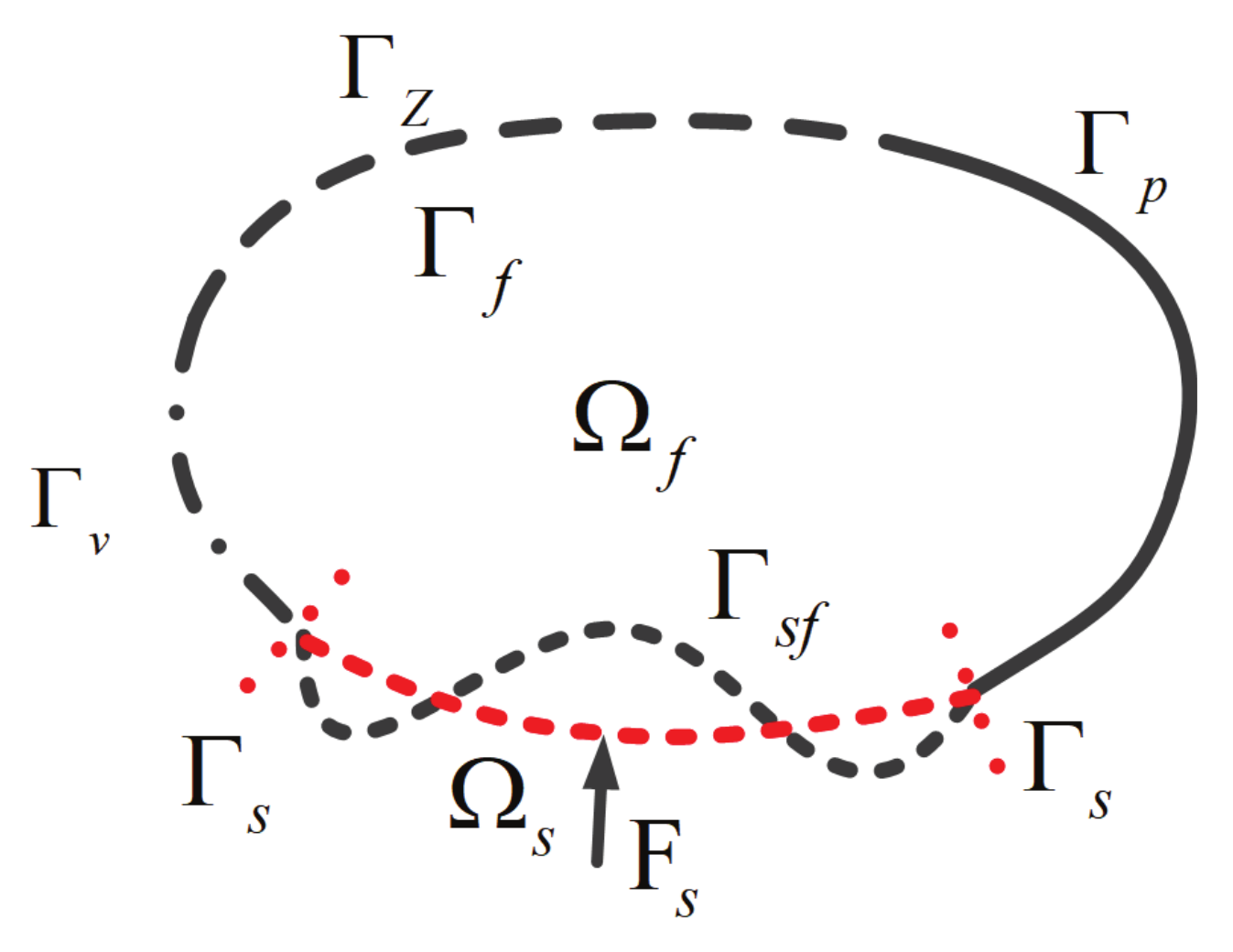
2. Formulation of Vibro-Acoustic Coupling System with Uncertain-But-Bounded Parameters

2.1. Interval Vibro-Acoustic Coupling Equation

For a deterministic interior coupled vibro-acoustic system, as shown in Figure 1, the structure, fluid, and coupling are, respectively, described with the following governing equations [31].

$$\begin{array}{c}\hfill {\nabla }^{\top }{\sigma }_s+{\mathbf{F}}_s={\rho }_s\frac{{\partial }^2{w}_s}{\partial t^2}{\mathsf{\Omega }}_s,{\mathsf{\Gamma }}_s\end{array}$$

(1)

$$\begin{array}{c}\hfill \frac{{\partial }^{2}p}{{\partial }^{2}t}-c_0^2{\nabla }^{2}p=0{\mathsf{\Omega }}_f,{\mathsf{\Gamma }}_f\end{array}$$

(2)

$$\begin{array}{c}\hfill \begin{array}{cc}{\left.w_s\right|}_n={\left.w_f\right|}_n& {\mathsf{\Gamma }}_{fs}\\ {\left.{\sigma }_s\right|}_n=-p& {\mathsf{\Gamma }}_{fs}\end{array}\end{array}$$

(3)

where ${\sigma }_s,{\mathbf{F}}_s$ represent stresses and external force respectively, $w_s,p$ denote the deflection and sound pressure, the subscript n denotes the outward normal direction, and ${\rho }_s,c_0$ represent the density of structures and sound speed of acoustic fluid, respectively. The boundary of fluid subsystem can be divided into two categories, one is the original acoustic boundary denoted as ${\mathsf{\Gamma }}_f$, which includes three types in detail, the pressure boundary (Dirichlet boundary) ${\mathsf{\Gamma }}_p$, the velocity boundary (Neumann boundary) ${\mathsf{\Gamma }}_v$, and the impedance boundary (Robin boundary) ${\mathsf{\Gamma }}_Z$.

As a matter of fact, the interaction between structure and acoustic can be simplified as the additional boundary conditions, respectively [32]. One of the effects from structural bending vibration can be regarded as the velocity boundary for acoustic, while the other is acoustic influence to structure, regarded as the stress boundary condition. If neglecting the damping of structure and the impedance boundary of acoustic domain, after the finite-element discretization, the coupling process would be described with the following formulations [32].

$$\begin{array}{c}\hfill \left({\mathbf{K}}_s-{\omega }^2·{\mathbf{M}}_s\right) · {\mathbf{w}}_s-{\mathbf{R}}_{cp}·{\mathbf{p}}_a={\mathbf{F}}_s\end{array}$$

(4)

$$\begin{array}{c}\hfill \left({\mathbf{K}}_a-{\omega }^2·{\mathbf{M}}_a\right) · \left\{p_j\right\} - {\rho }_a{\omega }^2·{\mathbf{R}}_{cp}^{\top }\left\{w_i\right\} = {\mathbf{F}}_a^v+{\mathbf{F}}_a^p\end{array}$$

(5)

$$\begin{array}{c}\hfill {\mathbf{R}}_{cp}={\int }_{{\mathsf{\Gamma }}_{sf}}{\mathbf{N}}_s^{\top }{\mathbf{n}}_f{\mathbf{N}}_{a}d\mathsf{\Omega }\end{array}$$

(6)

$$\begin{array}{c}\hfill {\mathbf{F}}_a^v={\int }_{{\mathsf{\Gamma }}_v}\left(-\mathrm{j}{\rho }_a\omega {\left\{N_i\right\}}_a{v}_n\right) · d\mathsf{\Omega }\end{array}$$

(7)

$$\begin{array}{c}\hfill {\mathbf{F}}_a^p={\int }_{{\mathsf{\Gamma }}_p}\left(-\mathrm{j}{\rho }_a\omega {\left\{N_i\right\}}_a\mathbf{v}·{\mathbf{n}}_f\right) · d\mathsf{\Omega }\end{array}$$

(8)

where ${\mathbf{K}}_s,{\mathbf{M}}_s,{\mathbf{K}}_a,{\mathbf{M}}_a$ represent stiffness and mass matrix for structure and acoustic, respectively, and ${\rho }_a$ is the density of acoustic fluid inside the cavity. When considering the velocity and pressure boundaries, the corresponding loads are defined with input velocity load $v_n$ on ${\mathbf{F}}_a^v$ and input pressure load ${\mathbf{F}}_a^p$. By employing the coupling matrix ${\mathbf{R}}_{cp}$ for two-way coupling, Equations (4)–(8) can be rewritten into a non-symmetrical form.

$$\left\{\left[\begin{array}{cc}{\mathbf{K}}_s& -{\mathbf{R}}_{cp}\\ \mathbf{0}& {\mathbf{K}}_a\end{array}\right]- {\omega }^2\left[\begin{array}{cc}{\mathbf{M}}_s& \mathbf{0}\\ {\rho }_a{\mathbf{R}}_{cp}^{\top }& {\mathbf{M}}_a\end{array}\right]\right\}\left\{\begin{array}{c}{\mathbf{w}}_s\hfill \\ {\mathbf{p}}_a\hfill \end{array}\right\} = \left\{\begin{array}{c}{\mathbf{F}}_s\hfill \\ {\mathbf{F}}_a\hfill \end{array}\right\}$$

(9)

If the density of fluid is light as air, it is apparently that the effect by structure plays the leading role to the interaction. Assuming that the interval uncertain properties are mainly assembled in structure, and then the structure is subject to uncertain variability, Equation (9) is transferred into the new form to analyze the uncertain vibro-acoustic coupling system.

$$\begin{array}{c}\hfill \begin{array}{cc}& {\mathbf{Z}}^I·{\mathbf{P}}^I={\mathbf{F}}^I\hfill \\ & {\mathbf{Z}}^I= \left[\begin{array}{cc}{\mathbf{K}}_s^I-{\omega }^2{\mathbf{M}}_s^I& -{\mathbf{R}}_{cp}\\ -{\rho }_a{\omega }^2{\mathbf{R}}_{cp}^{\top }& {\mathbf{K}}_a-{\omega }^2{\mathbf{M}}_a\end{array}\right]\hfill \\ & {\mathbf{P}}^I= \left\{\begin{array}{c}{\mathbf{w}}_s^I\hfill \\ {\mathbf{p}}_a^I\hfill \end{array}\right\};{\mathbf{F}}^I= \left\{\begin{array}{c}{\mathbf{F}}_s^I\hfill \\ {\mathbf{F}}_a\hfill \end{array}\right\}\hfill \end{array}\end{array}$$

(10)

where both the global matrices for structure ${\mathbf{K}}_s^I,{\mathbf{M}}_s^I,{\mathbf{F}}_s^I$ and response ${\mathbf{w}}_s^I,{\mathbf{p}}_a^I$ become the interval quantities with respect to the interval parameters ${\mathbf{u}}^I$, and then the uncertainties can be expressed as the n-dimensional closed interval vector with the equivalent form of midpoint value and maximum width,

$$\begin{array}{c}\hfill \begin{array}{cc}\hfill {\mathbf{u}}^I=[\underline{\mathbf{u}},\overline{\mathbf{u}}]& ={\left(u_i^I\right)}_n={\left\{u_i^c+ \left[-\Delta u_i,\Delta u_i\right]\right\}}_n\hfill \\ & ={\mathbf{u}}^c+[-\Delta \mathbf{u},\Delta \mathbf{u}]\hfill \\ & ={\mathbf{u}}^c+\Delta {\mathbf{u}}^{I}i=1,2\dots n\hfill \end{array}\end{array}$$

(11)

2.2. Unimodal Components’ Decomposition for Uncertain Structures

Since Chen introduced the Taylor series expansion in interval analysis [33,34], the Taylor series expanding method has become the most widely used tool in perturbation-based IFEMs, but it suffers from the non-conservative approximation for neglecting high-order terms in Neumann series expansion [8]. An alternative tracing method originates from the unimodal components’ decomposition [12,13], which can be also regarded as the practice to the suggestion of uncertainty factorization proposed by Köylüoğlu [35]. With the Sherman–Morrison–Woodbury series expansion [13], the previous concept of unimodal components’ decomposition is derived from the approximate explicit solutions of structural mechanics. Moreover, the basic and simple element expressions such as truss, space frame, and 2D constant strain triangle have been provided in literature [13,36] with explicit formulas. In order to build the “plate-cavity coupling model”, MITC4 (four-node mixed interpolation of tensorial components) for bending plate element [37] would be derived with approximate formulas by the proposed “generalized unimodal components’ decomposition” method. Here, using $E,{\rho }_s,h,v$ as the Young’s modulus, density, thickness of plate, and Poisson’s ratio for material, the MITC4 element can be decomposed as follows with Gaussian integration.

$$\begin{array}{c}\hfill \begin{array}{cc}\hfill {\mathbf{K}}_e^I=& \sum _{s=1}^N\sum _{t=1}^N\left(\begin{array}{c}{\mathbf{B}}_b^{\top }\left({\xi }_s,{\eta }_t\right){\mathbf{D}}_b{\mathbf{B}}_b\left({\xi }_s,{\eta }_t\right)\\ +{\mathbf{B}}_s^{\top }\left({\xi }_s,{\eta }_t\right){\mathbf{D}}_s{\mathbf{B}}_s\left({\xi }_s,{\eta }_t\right)\end{array}\right)w_{st}{J}_{st}\hfill \\ & ={\mathbf{A}}_{ke}diag\left({\mathbf{\Lambda }}_{ke}{\mathbf{\alpha }}_k^I\right){\mathbf{A}}_{ke}^{\top }\hfill \\ & = \left\{{\mathbf{A}}_{ke}^1\left({\xi }_1,{\eta }_1\right)\cdots {\mathbf{A}}_{ke}^{N\times N}\left({\xi }_N,{\eta }_N\right)\right\}\hfill \\ & ·diag\left(\left(\begin{array}{c}{\mathbf{\Lambda }}_{ke}^1\left({\xi }_1,{\eta }_1\right)\\ ⋮\\ {\mathbf{\Lambda }}_{ke}^{N\times N}\left({\xi }_N,{\eta }_N\right)\end{array}\right){\mathbf{\alpha }}_k^I\right) · \left\{\begin{array}{c}{\mathbf{A}}_{ke}^1{\left({\xi }_1,{\eta }_1\right)}^{\top }\\ ⋮\\ {\mathbf{A}}_{ke}^{N\times N}{\left({\xi }_N,{\eta }_N\right)}^{\top }\end{array}\right\}\hfill \end{array}\end{array}$$

(12)

$$\begin{array}{c}\hfill \begin{array}{cc}& {\mathbf{A}}_{ke}^i={\left\{\begin{array}{c}{\mathbf{B}}_b\left({\xi }_s,{\eta }_t\right)\hfill \\ {\mathbf{B}}_s\left({\xi }_s,{\eta }_t\right)\hfill \end{array}\right\}}^{\top }\left[\begin{array}{c}1,0,0,0,0\hfill \\ v,1,0,0,0\hfill \\ 0,0,1,0,0\hfill \\ 0,0,0,1,0\hfill \\ 0,0,0,0,1\hfill \end{array}\right]\sqrt{w_{st}{J}_{st}}\hfill \\ & {\mathbf{\Lambda }}_{ke}^i={\left\{\begin{array}{c}\frac{1}{12\left(1-v^2\right)},\frac{1}{12},\frac{1}{24(1+v)},0,0\\ 0,0,0,\frac{\kappa }{2(1+v)},\frac{\kappa }{2(1+v)}\end{array}\right\}}^{\top },{\mathbf{\alpha }}_k^I={\left[E{h}^3,Eh\right]}^{\top }\hfill \end{array}\end{array}$$

(13)

$$\begin{array}{c}\hfill {\mathbf{B}}_b= \left[\begin{array}{ccccc}& 0& N_{i,x}& 0& \\ \cdots & 0& 0& N_{i,y}& \cdots \\ & 0& N_{i,y}& N_{i,x}\end{array}\right],\left\{\begin{array}{c}{N}_{i,x}\hfill \\ N_{i,y}\hfill \end{array}\right\} = \mathbf{J}· \left\{\begin{array}{c}{N}_{i,\xi }\hfill \\ N_{i,\eta }\hfill \end{array}\right\}i=1,2,3,4\end{array}$$

(14)

$$\begin{array}{c}\hfill \begin{array}{cc}& {\mathbf{B}}_s=1/8·{\mathbf{J}}^{-1}{\mathbf{N}}_{\gamma }{\mathbf{A}}_{\gamma }\hfill \\ & {\mathbf{N}}_{\gamma }= \left[\begin{array}{c}\frac{1}{2}(1-\eta ),0,\frac{1}{2}(1+\eta ),0\hfill \\ 0,\frac{1}{2}(1+\xi ),0,\frac{1}{2}(1-\xi )\hfill \end{array}\right]\hfill \\ & {\mathbf{A}}_{\gamma }= \left[\begin{array}{cccccccccccc}-2& -x_{12}& -y_{12}& 2& -x_{12}& -y_{12}& 0& 0& 0& 0& 0& 0\\ 0& 0& 0& -2& -x_{23}& -y_{23}& 2& -x_{23}& -y_{23}& 0& 0& 0\\ 0& 0& 0& 0& 0& 0& 2& x_{34}& y_{34}& -2& x_{34}& y_{34}\\ -2& x_{41}& y_{41}& 0& 0& 0& 0& 0& 0& 2& x_{41}& y_{41}\end{array}\right]\hfill \end{array}\end{array}$$

(15)

$$\begin{array}{c}\hfill \begin{array}{cc}& {\mathbf{D}}_b=\frac{E{h}^3}{12\left(1-v^2\right)}\left[\begin{array}{ccc}1& v& 0\\ v& 1& 0\\ 0& 0& (1-v)/2\end{array}\right]\hfill \\ & {\mathbf{D}}_s=\frac{\kappa Eh}{2(1+v)}\left[\begin{array}{cc}1\hfill & 0\hfill \\ 0\hfill & 1\hfill \end{array}\right]\hfill \end{array}\end{array}$$

(16)

$$\begin{array}{c}\hfill \begin{array}{cc}\hfill {\mathbf{M}}_e^I=& \sum _{s=1}^N\sum _{t=1}^N\left({\mathbf{N}}_m^{\top }\left({\xi }_s,{\eta }_t\right){\mathbf{I}}_m{\mathbf{N}}_m\left({\xi }_s,{\eta }_t\right)\right)w_{st}{J}_{st}\hfill \\ & ={\mathbf{A}}_{me}diag\left({\mathbf{\Lambda }}_{me}{\mathbf{\alpha }}_m^I\right){\mathbf{A}}_{me}^{\top }\hfill \\ & = \left\{{\mathbf{A}}_{me}^1\left({\xi }_1,{\eta }_1\right)\cdots {\mathbf{A}}_{me}^{N\times N}\left({\xi }_N,{\eta }_N\right)\right\}\hfill \\ & ·diag\left(\left(\begin{array}{c}{\mathbf{\Lambda }}_{me}^1\left({\xi }_1,{\eta }_1\right)\\ ⋮\\ {\mathbf{\Lambda }}_{me}^{N\times N}\left({\xi }_N,{\eta }_N\right)\end{array}\right){\mathbf{\alpha }}_m^I\right) · \left\{\begin{array}{c}{\mathbf{A}}_{me}^1{\left({\xi }_1,{\eta }_1\right)}^{\top }\\ ⋮\\ {\mathbf{A}}_{me}^{N\times N}{\left({\xi }_N,{\eta }_N\right)}^{\top }\end{array}\right\}\hfill \end{array}\end{array}$$

(17)

$$\begin{array}{c}\hfill \begin{array}{cc}& {\mathbf{A}}_{\mathrm{me}}^i={\mathbf{N}}_m^{\top }\sqrt{w_{st}{J}_{st}}= \left[\begin{array}{c}{N}_1,0,0,N_2,0,0,N_3,0,0,N_4,0,0\\ 0,N_1,0,0,N_2,0,0,N_3,0,0,N_4,0\\ 0,0,N_1,0,0,N_2,0,0,N_3,0,0,N_4\end{array}\right]\sqrt{w_{st}{J}_{st}}\hfill \\ & {\mathbf{\Lambda }}_{me}^i={\left\{\begin{array}{ccc}1& 0& 0\\ 0& 1/12& 1/12\end{array}\right\}}^{\top }{\rho }_s,{\mathbf{\alpha }}_m^I={\left[\begin{array}{c}h,h^3\hfill \end{array}\right]}^{\top }\hfill \end{array}\end{array}$$

(18)

$$\begin{array}{c}\hfill {\mathbf{I}}_m= \left[\begin{array}{ccc}\rho h& 0& 0\\ 0& \rho h^3/12& 0\\ 0& 0& \rho h^3/12\end{array}\right]\end{array}$$

(19)

where ${\mathbf{A}}_{ke},{\mathbf{A}}_{me},{\mathbf{\Lambda }}_{ke},{\mathbf{\Lambda }}_{me}$ are deterministic matrices, ${\mathbf{\alpha }}_k^I,{\mathbf{\alpha }}_m^I$ are uncertain vectors, $w_{st},J_{st}$ represent weight and Jacob’s ratio of the Gaussian integral method, ${\xi }_s,{\eta }_t$ are both the corresponding Gaussian integral points for two-dimensional case, $\kappa$ is the shear correction factor (usually 5/6 for an isotropic homogeneous plate), and ${\mathbf{I}}_m$ is the inertia matrix in Ressiner–Mindlin plate theory. The representations $x_{ij},y_{ij}$ in Equation (15) are simplified for the formula $x_{ij}=x_i-x_j,y_{ij}=y_i-y_j$.

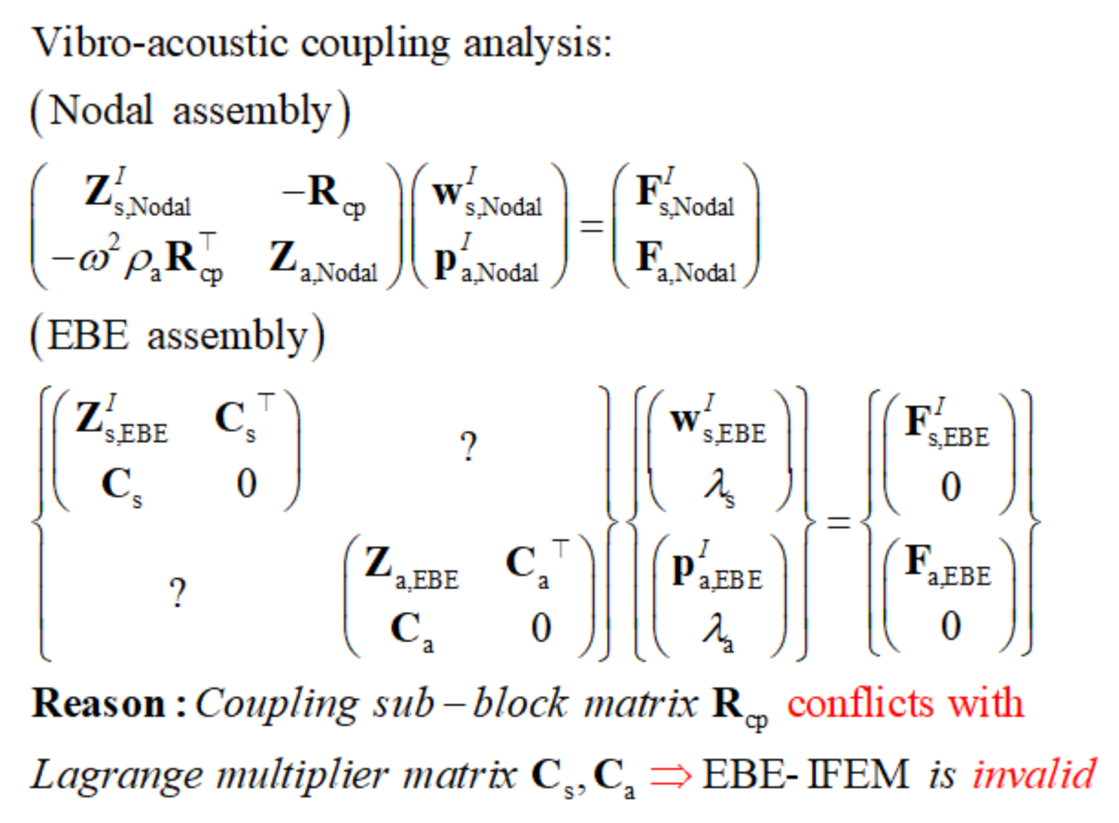
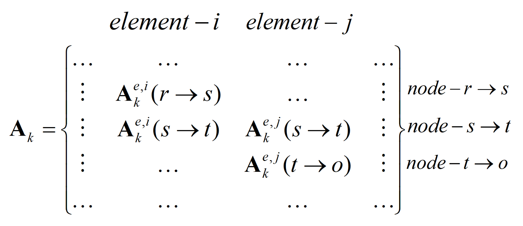
2.3. Different Assembly Strategies for Interval Coupling System

As the abovementioned in Section 1, the EBE-IFEM cannot be applied in vibro-acoustic analysis, and the direct explanation for the problem is shown in Figure 2. As the Lagrange multiplier in element-by-element assemblage is incompatible with the coupling sub-block matrix, the application of the EBE-IFEM is restricted to uncoupled problem [11]. To deal with this dilemma, the assemblage of element-by-element should be replaced by another one with the attributes of nodal indexes, so that the modified interval arithmetic approach would be applicable in the coupling problem. As expected, the answer is found in the unimodal components’ analysis as well [12,13]. Subsequently, in order to distinguish the referred three methods of elemental assembly, apart from the traditional nodal assemblage and element-by-element type, the new one is named with the mixed-nodal-element assemblage (MNE) [12] because this new assembly method has adopted their technical advantages, not only satisfying the coupling equation but also applying to the factorization of uncertainties. In addition, it may save the computational cost with the reduced model, in contrast to EBE-IFEM, when solving the uncoupled field.

As per the above analysis, the effective assembly methods for coupling problem are the nodal assembly method and the mixed-nodal-element assemblage. The detail of the mixed-nodal-element assembling is depicted in Figure 3 for the general case of ${\mathbf{A}}_k^{e,i}$ to ${\mathbf{A}}_k$ assembling. In brief, each line-vector of the deterministic matrix ${\mathbf{A}}_k^{e,i}$ should be assembled by the nodal index similar to the traditional nodal assemblage, but each column-vector of ${\mathbf{A}}_k^{e,i}$ should be assembled by element index similar to the EBE-assemblage. For the other deterministic matrix ${\mathbf{\Lambda }}_k^i$, it is the same as the element-by-element type [38]; the system matrix ${\mathbf{\Lambda }}_k$ with N sub-matrices is assembled as

$$\begin{array}{c}\hfill {\mathbf{\Lambda }}_k= \left[\begin{array}{ccc}{\mathbf{\Lambda }}_k^1;\hfill & \cdots \hfill & ;{\mathbf{\Lambda }}_k^N\hfill \end{array}\right]\end{array}$$

(20)

Observing the different methodologies in the preprocessing phase, it is instructive to clarify the logic and relationship among the different IFEMs applied to the vibro-acoustic coupling problem. As shown in Figure 4, the existing methods for the coupling problem can be sorted into two classes: the perturbation-based method and the modified interval arithmetic strategy. With the two types of uncertain tracing means and assembly ways, the next step is to give an approximation of the inverse corresponding to the interval matrix. Referring to Neumann series approximation, SMW series approximation, and iterative enclosure solution, three kinds of IFEMs are finally established theoretically. The point to emphasize here is that the TN-MIPFEM is inspired by the SMW-IPFEM with two reasons [8,21,22]: on one hand, the SMW-IPFEM creatively provides a special Neumann series expansion to retain more high-order terms of the non-conservative approximation [21]; on the other hand, the interval-value SMW approximation is confined to the specific dyadic-product formula [8,21,22], which hinders the dynamic application of SMW-IPFEM.

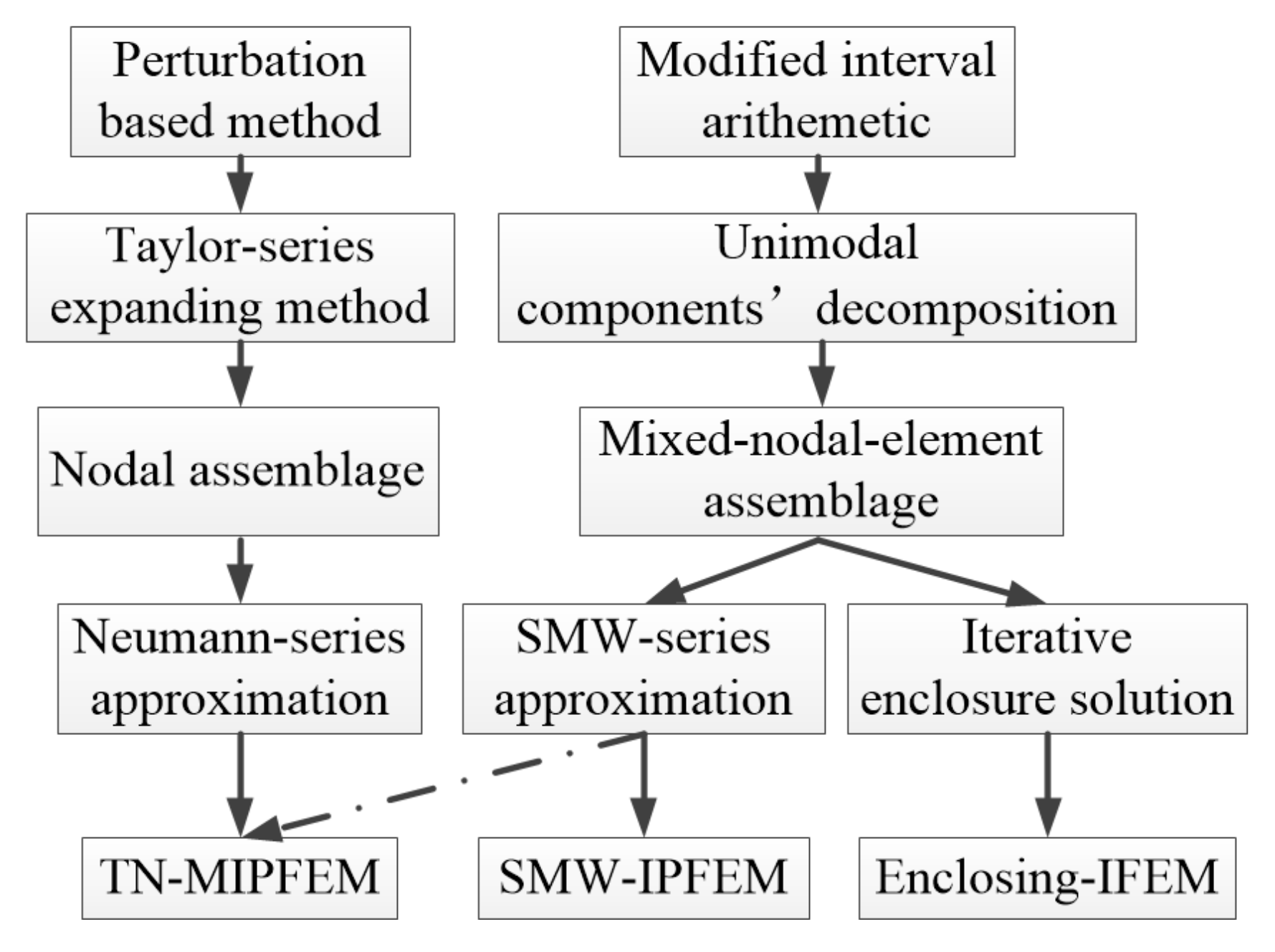
2.4. The Construction of the Interval Coupling Governing Equations

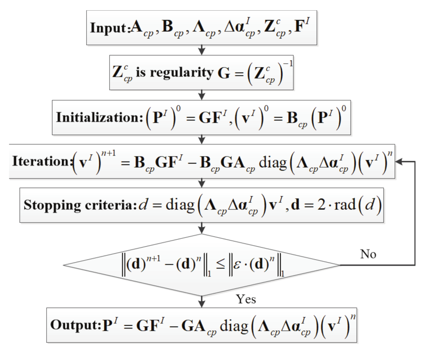
2.4.1. The Iterative Enclosure Formula of Interval Coupling Governing Equations

In Section 2.2, the decompositions of stiffness and mass matrices were given. By the mixed-nodal-element assemblage (MNE) referred to in Section 2.3, the decomposition after assembling becomes

$$\begin{array}{c}\hfill \begin{array}{cc}& {\mathbf{K}}_{\mathrm{MNE}}^I={\mathbf{A}}_{k}diag\left({\mathbf{\Lambda }}_k{\mathbf{\alpha }}_k^I\right){\mathbf{A}}_k^{\top }={\mathbf{K}}^I\hfill \\ & {\mathbf{M}}_{\mathrm{MNE}}^I={\mathbf{A}}_{m}diag\left({\mathbf{\Lambda }}_m{\mathbf{\alpha }}_m^I\right){\mathbf{A}}_m^{\top }={\mathbf{M}}^I\hfill \end{array}\end{array}$$

(21)

where ${\mathbf{K}}_{\mathrm{MNE}}^I$ and ${\mathbf{M}}_{\mathrm{MNE}}^I$ with mixed-nodal-element assemblage are equal to the ${\mathbf{K}}^I$ and ${\mathbf{M}}^I$ with traditional nodal assemblage, respectively.

Supposing that the uncertainty is just restricted in structures and no damping is taken into account, by the same method as EBE-IFEM, the interval dynamic stiffness matrix is expressed with the formula similar to the generalized unimodal components’ decomposition,

$$\begin{array}{c}\hfill \begin{array}{cc}& {\mathbf{D}}_s^I={\mathbf{A}}_{s}diag\left({\mathbf{\Lambda }}_s{\mathbf{\alpha }}_s^I\right){\mathbf{B}}_s\hfill \\ & {\mathbf{A}}_s= \left\{{\mathbf{A}}_k,-{\omega }^2{\mathbf{A}}_m\right\}\hfill \\ & {\mathbf{\Lambda }}_s= \left\{\begin{array}{cc}{\mathbf{\Lambda }}_k& 0\\ 0& {\mathbf{\Lambda }}_m\end{array}\right\}\hfill \\ & {\mathbf{\alpha }}_s^I= \left\{{\mathbf{\alpha }}_k^I;{\mathbf{\alpha }}_m^I\right\},{\mathbf{B}}_s={\left\{{\mathbf{A}}_k,{\mathbf{A}}_m\right\}}^{\top }\hfill \end{array}\end{array}$$

(22)

where ${\mathbf{A}}_s,{\mathbf{\Lambda }}_s,{\mathbf{B}}_s$ are all deterministic matrices for the coupling system, and the uncertainties are only isolated in ${\mathbf{\alpha }}_s^I$.

Then, substituting ${\mathbf{D}}_s^I$ to Equation (10), the coupling equation is equivalent to

$$\begin{array}{c}\hfill \left[\begin{array}{cc}{\mathbf{D}}_s^I& -{\mathbf{R}}_{cp}\\ -{\rho }_a{\omega }^2{\mathbf{R}}_{cp}^{\top }& {\mathbf{K}}_a-{\omega }^2{\mathbf{M}}_a\end{array}\right]{\mathbf{P}}^I={\mathbf{F}}^I\end{array}$$

(23)

Since only ${\mathbf{D}}_s^I$ is uncertain in the dynamic matrix ${\mathbf{Z}}^I$, by introducing the centered-form from Equation (11), ${\mathbf{\alpha }}_s^I={\mathbf{\alpha }}_s^c+\Delta {\mathbf{\alpha }}_s^I$, the coupling Equation (23) can be transformed into

$$\begin{array}{c}\hfill \begin{array}{cc}& \left\{\left[\begin{array}{cc}{\mathbf{D}}_s^c& -{\mathbf{R}}_{cp}\\ -{\rho }_a{\omega }^2{\mathbf{R}}_{cp}^{\top }& {\mathbf{K}}_a-{\omega }^2{\mathbf{M}}_a\end{array}\right]+ {\mathbf{A}}_{cp}diag\left({\mathbf{\Lambda }}_{cp}\Delta {\mathbf{\alpha }}_{cp}^I\right){\mathbf{B}}_{cp}\right\}{\mathbf{P}}^I={\mathbf{F}}^I\hfill \end{array}\end{array}$$

(24)

$$\begin{array}{c}\hfill \begin{array}{cc}& {\mathbf{A}}_{cp}= \left\{\begin{array}{c}{\mathbf{A}}_s\\ 0\end{array}\right\};{\mathbf{B}}_{cp}= \left\{\begin{array}{cc}{\mathbf{B}}_s\hfill & 0\hfill \end{array}\right\}\hfill \\ & {\mathbf{\Lambda }}_{cp}={\mathbf{\Lambda }}_s;\Delta {\mathbf{\alpha }}_{cp}^I=\Delta {\mathbf{\alpha }}_s^I\hfill \end{array}\end{array}$$

(25)

Further defining the deterministic matrix in Equation (24) as ${\mathbf{Z}}_{cp}^c$, it can be rewritten with simplified formula, which is called iterative enclosure formula [14]:

$$\begin{array}{c}\hfill \left({\mathbf{Z}}_{cp}^c+{\mathbf{A}}_{cp}diag\left({\mathbf{\Lambda }}_{cp}\Delta {\mathbf{\alpha }}_{cp}^I\right){\mathbf{B}}_{cp}\right){\mathbf{P}}^I={\mathbf{F}}^I\end{array}$$

(26)

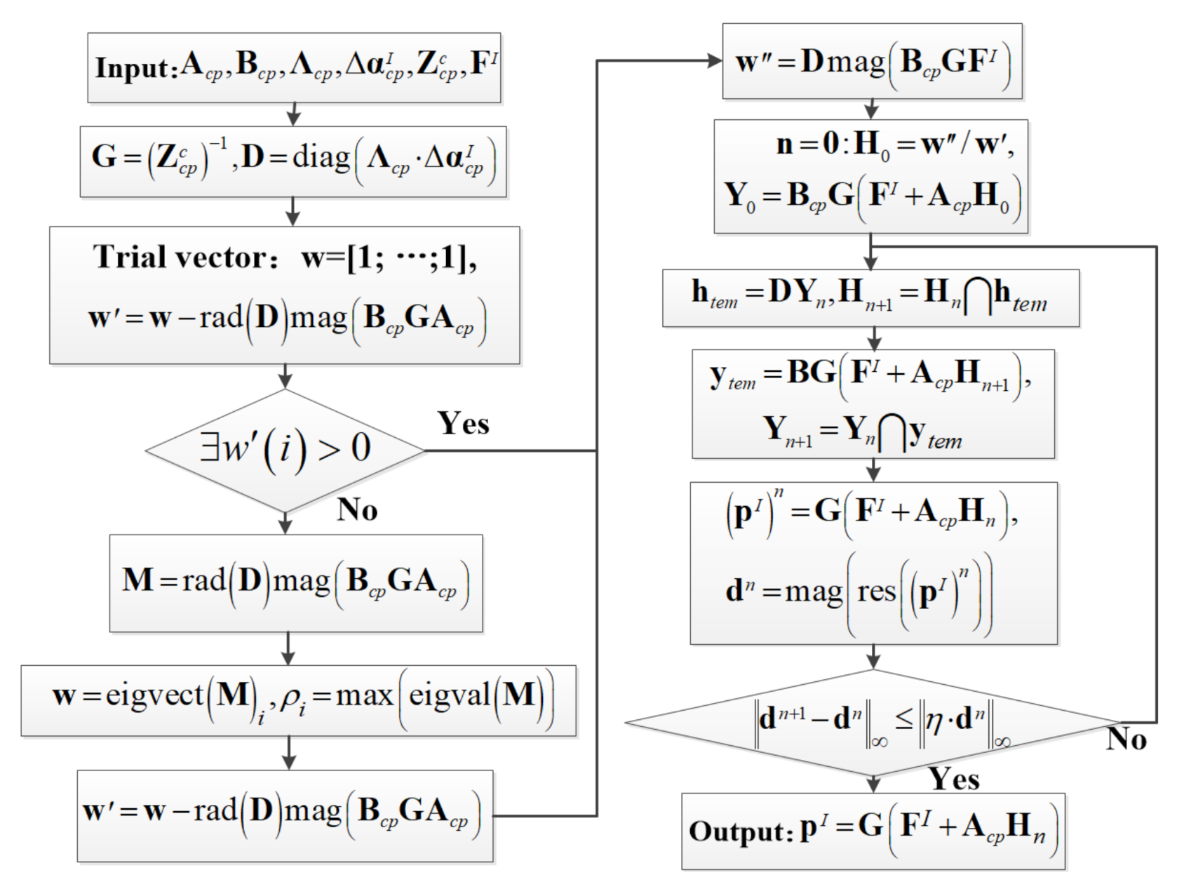
2.4.2. The Dyadic-Product Formula of Interval Coupling Governing Equation for the Dynamic Extended SMW-IPFEM

As Xia [8,22] pointed out, with the difficulty to derive the dyadic-product expressions in dynamic analysis, the application of SMW-IPFEM [30] is restricted in static analysis. However, in order to extend the SMW-IPFEM to vibro-acoustic analysis or dynamic analysis, the formula of dyadic-product can be derived from the iterative enclosure Equation (26) with the proposed mixed-nodal-element assemblage.

$$\begin{array}{c}\hfill \begin{array}{cc}& \left({\mathbf{Z}}_{cp}^c+\sum _{i=1}^r{\gamma }_i^I{\mathbf{a}}_i{\mathbf{b}}_i\right){\mathbf{P}}^I={\mathbf{F}}^I\hfill \\ & {\gamma }^I=diag\left({\mathbf{\Lambda }}_{cp}\Delta {\mathbf{\alpha }}_s^I\right) =diag\left(\begin{array}{ccc}{\gamma }_1^I\hfill & \cdots \hfill & {\gamma }_r^I\hfill \end{array}\right)\hfill \\ & {\mathbf{A}}_{cp}= \left[\begin{array}{ccc}{\mathbf{a}}_1,\hfill & \cdots \hfill & ,{\mathbf{a}}_r\hfill \end{array}\right]\hfill \\ & {\mathbf{B}}_{cp}= \left[\begin{array}{ccc}{\mathbf{b}}_1;\hfill & \cdots \hfill & ;{\mathbf{b}}_r\hfill \end{array}\right]\hfill \end{array}\end{array}$$

(27)

Apparently, based on the dyadic-product Equation (27) and solution expressions of SMW-IPFEM [30], it is possible for SMW-IPFEM to calculate the approximated upper and lower bounds of ${\mathbf{P}}^I$. Thus, the applied theory for the SMW-IPFEM in vibro-acoustic analysis is perfected.

3. Enclosing Interval Finite-Element Method for Coupling Problem

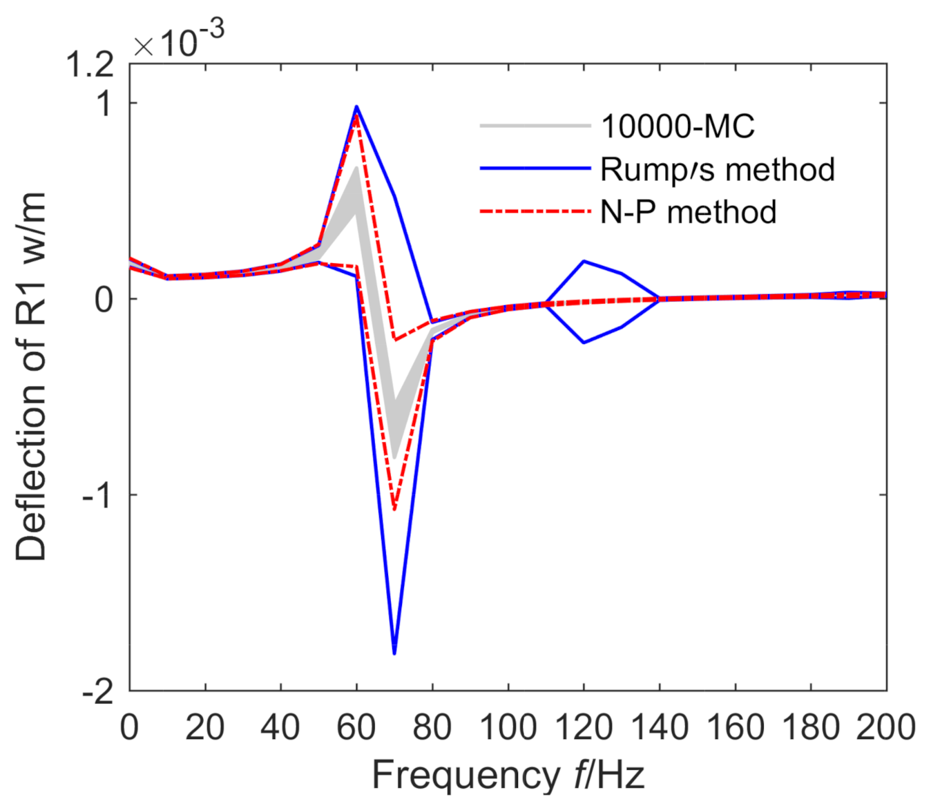
3.1. Rump’s Inclusion Method in Vibro-Acoustic Coupling Problem

In order to confine the overestimation of results, Rump’s inclusion method is developed by employing the fixed point theorem [7] to solve the interval uncertain system. Based on the fixed point theorem [15,38], Equation (26) can be also rewritten as the fixed point form,

$$\begin{array}{c}\hfill {\mathbf{Z}}_{cp}^c{\mathbf{P}}^I={\mathbf{F}}^I-{\mathbf{A}}_{cp}diag\left({\mathbf{\Lambda }}_{cp}\Delta {\mathbf{\alpha }}_{cp}^I\right){\mathbf{B}}_{cp}{\mathbf{P}}^I\end{array}$$

(28)

For practice, the Rump’s inclusion method procedure is illustrated with a flow chart, given in Figure 5. Apparently, the matrix ${\mathbf{Z}}_{cp}^c$ is non-singular and invertible by means of physical problem at the midpoint value of parametric interval. Therefore, with the special definition $\mathbf{G}={\left({\mathbf{Z}}_{cp}^c\right)}^{-1}$, ${\mathbf{P}}^I$ satisfies the fixed point form, as follows:

$$\begin{array}{cc}\hfill {\left({\mathbf{P}}^I\right)}^{n+1}& =\mathbf{G}{\mathbf{F}}^I-\mathbf{G}{\mathbf{A}}_{cp}·diag\left({\mathbf{\Lambda }}_{cp}\Delta {\mathbf{\alpha }}_{cp}^I\right){\mathbf{B}}_{cp}{\left({\mathbf{P}}^I\right)}^n\end{array}$$

(29)

Although the approximate solution set can be figured out by Equation (29), the accuracy of interval may be influenced by the redundant intermediate operation ${\mathbf{B}}_{cp}\left({\mathbf{P}}^I\right)$ so that, with the auxiliary variable ${\mathbf{v}}^I={\mathbf{B}}_{cp}{\mathbf{P}}^I$, the iterative form is transformed into

$$\begin{array}{cc}\hfill {\left({\mathbf{v}}^I\right)}^{n+1}& ={\mathbf{B}}_{cp}\mathbf{G}{\mathbf{F}}^I-{\mathbf{B}}_{cp}\mathbf{G}{\mathbf{A}}_{cp}·diag\left({\mathbf{\Lambda }}_{cp}\Delta {\mathbf{\alpha }}_{cp}^I\right){\left({\mathbf{v}}^I\right)}^n\end{array}$$

(30)

In addition, two basic aspects need be under consideration for the iteration: one is the initial value and another is the stopping criteria. It has been verified by Xiao [36] that ${\mathbf{v}}^I={\mathbf{B}}_{cp}\mathbf{G}{\mathbf{F}}^I$ is feasible to be the initialization of iteration. Additional stopping criteria by employing convergence condition is given by

$$\begin{array}{c}\hfill \begin{array}{cc}& d=diag\left({\mathbf{\Lambda }}_{cp}\Delta {\mathbf{\alpha }}_{cp}^I\right){\mathbf{v}}^I\hfill \\ & \mathbf{d}= \left\{{\overline{d}}_i-{\underline{d}}_i\right\} =2·rad\left(d\right)\hfill \\ & {\parallel {\left(\mathbf{d}\right)}^{n+1}-{\left(\mathbf{d}\right)}^n\parallel }_1\le {∥\epsilon ·{\left(\mathbf{d}\right)}^n∥}_1\hfill \end{array}\end{array}$$

(31)

where $\mathbf{d}$ is a vector to represent the width of the given interval vector d. ${∥·∥}_1$ is the 1-norm of the vector, which represents the absolute sum of the elements of the vector. $\epsilon$ is the tolerance of the iteration. Assuming that after n times of steps, the output satisfies the stopping criteria, the final solution set is given by

$$\begin{array}{c}\hfill {\mathbf{P}}^I=\mathbf{G}{\mathbf{F}}^I-\mathbf{G}{\mathbf{A}}_{cp}diag\left({\mathbf{\Lambda }}_{cp}\Delta {\mathbf{\alpha }}_{cp}^I\right){\left({\mathbf{v}}^I\right)}^n\end{array}$$

(32)

Generally, the Rump’s inclusion method is functional to approach the actual interval with high accuracy (less than 10 times the steps). However, it should be pointed out that it would fail in some cases with large-scale dimension (the curse of dimensionality), even if the uncertain level is small [14]. As a consequence, it calls for another algorithm to ensure the convergence of iteration.

3.2. Neumaier–Pownuk Method in Vibro-Acoustic Coupling Problem

Although the parametric uncertain truss systems were analyzed by Neumaier [14] and Popova [39] in their respective research work, the application of iterative procedure constituted by the Neumaier–Pownuk method has not been widely accepted in interval finite-element analysis, due to lack of the generic finite-element framework to transform the interval parametric system into the specific interval linear equation (called the iterative enclosure formula).

To carry out the iteration of the Neumaier–Pownuk method, the following definitions should be given first. The radius $rad\left({\mathbf{u}}^I\right)$, the magnitude $mag\left({\mathbf{u}}^I\right)$ of an interval vector ${\mathbf{u}}^I$, and the residual of the approximate solution $res\left({\mathbf{x}}^{\ast }\right)$ of the interval uncertain linear system ${\mathbf{A}}^I{\mathbf{x}}^{\ast }={\mathbf{b}}^I$ are described by these formulas:

$$\begin{array}{c}\hfill \begin{array}{cc}\hfill rad\left({\mathbf{u}}^I\right)& = \left|\left({\mathbf{u}}^I-{\mathbf{u}}^c\right)\right|\hfill \\ \hfill mag\left({\mathbf{u}}^I\right)& = |{\mathbf{u}}^I| =max(\underline{\mathbf{u}},\overline{\mathbf{u}})\hfill \\ \hfill res\left({\mathbf{x}}^{\ast }\right)& ={\mathbf{b}}^I-{\mathbf{A}}^I{\mathbf{x}}^{\ast }\hfill \end{array}\end{array}$$

(33)

The flow chart of the Neumaier–Pownuk method is shown in Figure 6. The Neumaier–Pownuk method does not require strong regularity of the coefficient matrix ${\mathbf{Z}}_{cp}^c$, as long as the matrix is invertible, and $\mathbf{G}={\left({\mathbf{Z}}_{cp}^c\right)}^{-1}$ and defines the diagonal matrix as $\mathbf{D}$. Let the initial vector $\mathbf{w}$ be a unit vector, which means all the elements of the unit vector are equal to 1; then the trial vector becomes

$$\begin{array}{c}\hfill \begin{array}{cc}\hfill {\mathbf{w}}^{\prime }& =\mathbf{w}-rad\left(\mathbf{D}\right)mag\left({\mathbf{B}}_{cp}\mathbf{G}{\mathbf{A}}_{cp}\right)\hfill \\ \hfill {\mathbf{w}}^{″}& =\mathbf{D}mag\left({\mathbf{B}}_{cp}\mathbf{G}{\mathbf{F}}^I\right)\hfill \end{array}\end{array}$$

(34)

If there exists an entry in the trial vector greater than zero, the initial value of the iteration can be written as

$$\begin{array}{c}\hfill {\mathbf{H}}_0={\mathbf{w}}^{″}/{\mathbf{w}}^{\prime },{\mathbf{Y}}_0={\mathbf{B}}_{cp}\mathbf{G}\left({\mathbf{F}}^I+{\mathbf{A}}_{cp}{\mathbf{H}}_0\right)\end{array}$$

(35)

Otherwise, by the eigenvalue calculation, the eigenvector with respect to the largest one of eigenvalue takes place of $\mathbf{w}$, and participates in the initialization. Repeat the loop, until satisfying the stopping criteria; for the n steps’ intermediate results of ${\mathbf{H}}_n$, the iteration sometimes can be relaxed to ${\mathbf{h}}_{tem}$.

$$\begin{array}{c}\hfill \begin{array}{cc}& {\mathbf{h}}_{\mathrm{tem}}=\mathbf{D}{\mathbf{Y}}_n,{\mathbf{H}}_{n+1}={\mathbf{H}}_n\cap {\mathbf{h}}_{\mathrm{tem}}\hfill \\ & {\mathbf{y}}_{\mathrm{tem}}={\mathbf{B}}_{cp}\mathbf{G}\left({\mathbf{F}}^I+{\mathbf{A}}_{cp}{\mathbf{H}}_{n+1}\right),{\mathbf{Y}}_{n+1}={\mathbf{Y}}_n\cap {\mathbf{y}}_{\mathrm{tem}}\hfill \end{array}\end{array}$$

(36)

Distinguished from the Rump’s inclusion method and original Neumaier–Pownuk method, the truncation technique of residual is introduced to accelerate the iteration. In detail, the algorithm will stop when there is no further improvement for residual,

$$\begin{array}{c}\hfill \begin{array}{cc}& {\left({\mathbf{P}}^I\right)}^n=\mathbf{G}\left({\mathbf{F}}^I+{\mathbf{A}}_{cp}{\mathbf{H}}_n\right)\hfill \\ & {\mathbf{d}}^n=mag\left(res\left({\left({\mathbf{P}}^I\right)}^n\right)\right)\hfill \\ & {∥{\left(\mathbf{d}\right)}^{n+1}-{\left(\mathbf{d}\right)}^n∥}_{\infty }\le {∥\eta ·{\left(\mathbf{d}\right)}^n∥}_{\infty }\hfill \end{array}\end{array}$$

(37)

where the ${∥·∥}_{\infty }$ represents the maximum absolute value belonging to vector’s component, which is widely used in the iterative method.

In order to achieve optimal solution of the enclosing-IFEM, it is essential to make a quantitative analysis of the two iterative procedures, especially in the analysis of residual convergence, which is the key to guaranteeing the accuracy of the solution. For next section, the comparative study among three different IFEMs (TN-MIPFEM [21,22], the dynamic extended SMW-IPFEM [30], and enclosing-IFEM), focus on both the conservativeness of solution sets and the time cost of computation. All the numerical applications will be computed in the platform of Matlab version R2017a, together with the INTLAB version 12 toolbox [40] by a Intel 2.90-GHz Core CPU i5-9400F.

4. Numerical Applications in Vibro-Acoustic Coupling Problem

A comprehensive presentation of the general application by the proposed enclosing-IFEM is given by this section, which contains a two-dimensional vibro-acoustic coupling problem of the actual car and a vibro-acoustic coupling problem of the regular-shaped three-dimensional model. Damping is also neglected with the uncertainties only caused by the structure, thus the TN-MIPFEM, SMW-IPFEM, and enclosing-IFEM can all be applied to this type of coupling problem. If enough samples are available to approach the exact solution [9,22], with the cross-reference by Monte Carlo sampling of FEM, both the conservativeness and computational efficiency for the enclosing-IFEM can be obtained by comparative analysis in the fields of inclusion relations and computational time, respectively. As an illustration, if all the results of enclosing-IFEM in the following numerical applications are preformed by the better iterative algorithm “Neumaier–Pownuk method”, it will be specially verified in the subsection C with the analysis of residual convergence.

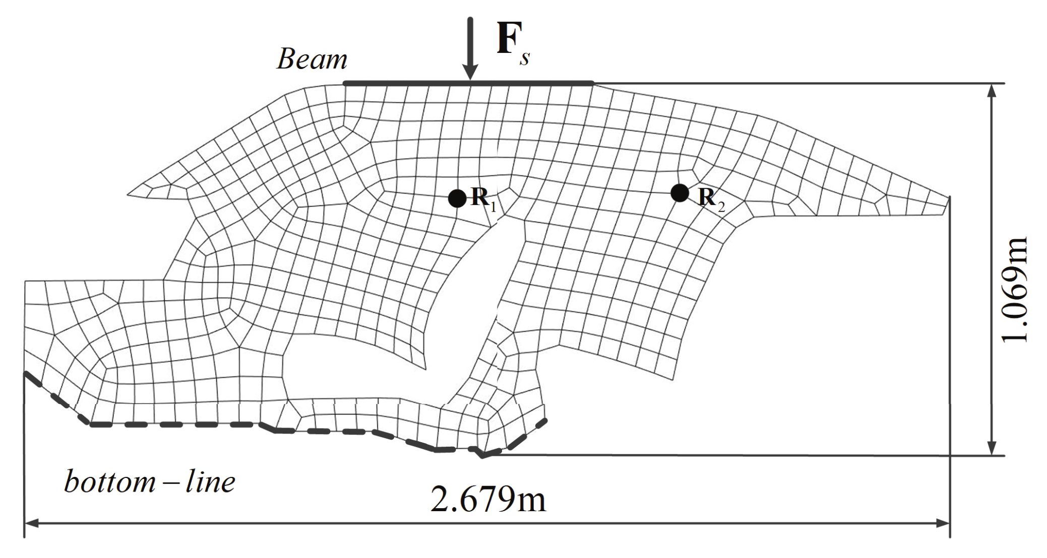
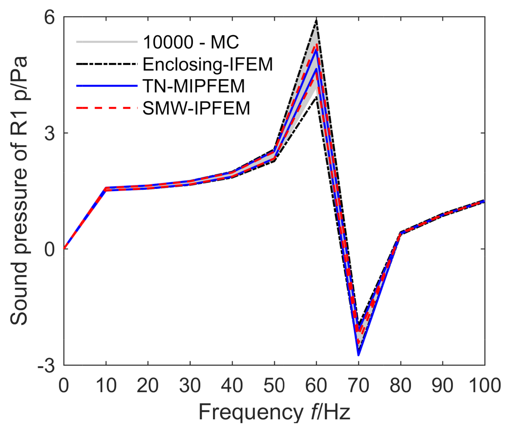
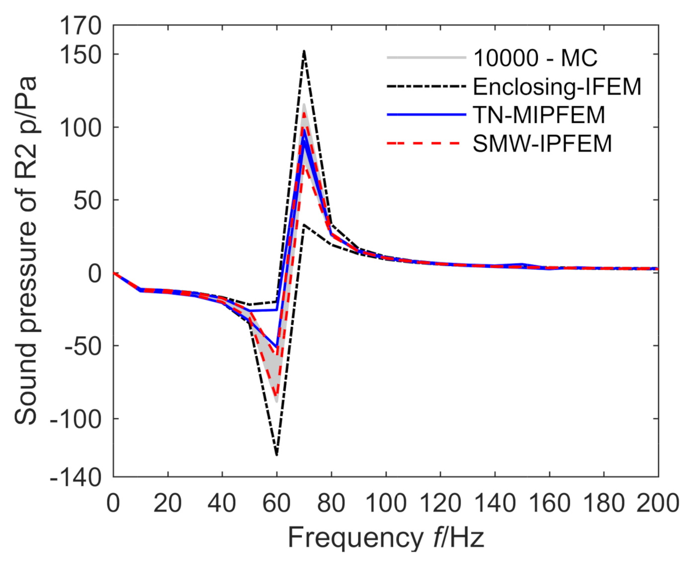
4.1. Numerical Analysis of a 2D Interior-Car Vibro-Acoustic Coupling Model

Few researchers have paid attention to the 2D uncertain vibro-acoustic coupling problem in previous literature [26], especially for the actual model with wide analytical band. The first application is implemented in 2D vibro-acoustic coupling system with uncertain-but-bounded parameters. As the prediction of a car’s interior-acoustic field is available as a benchmark problem in many uncoupled acoustical studies with uncertainties [8,21], it is valuable and innovative to characterize response of the 2D car’s acoustic field under the influence of the uncertain structural coupling. Figure 7 shows a 2D interior-acoustic field of a car, whose top face is attached to the simple support Euler beam (space frame [36]), and the remaining boundary of the acoustic field is supposed to be rigid. The vibro-acoustic coupling system is excited by a unit point load ${\mathbf{F}}_s$ on the midpoint of the beam. The beam is made by steel with material parameters $E=210\mathrm{Gpa},{\rho }_s=7800\mathrm{kg}/{\mathrm{m}}^3,\mu =0.3$, and the cross-section parameters $A=1\times {10}^{-5}{\mathrm{m}}^2\mathrm{and}I=8.3\times {10}^{-11}{\mathrm{m}}^4$. The cavity is filled with air with a density of ${\rho }_f=1.21\mathrm{kg}/{\mathrm{m}}^3$, and sound speed of $c=343\mathrm{m}/\mathrm{s}$. The number of elements and nodes corresponding to beam are 12 and 13, respectively, and to the acoustic domain become 501 and 579, respectively. Considering the unpredictability of structural parameters, the Young’s modulus E and density ${\rho }_s$ are assumed to be uncertain-but-bounded variables; with the preset uncertain level $\mathbf{\alpha }=0.05$, the uncertainties can be rewritten as

$$\begin{array}{c}\hfill \begin{array}{cc}& E^I=E^c+[-\mathbf{\alpha },\mathbf{\alpha }]\times E^c\hfill \\ & {\rho }_s^I={\rho }_s^c+[-\mathbf{\alpha },\mathbf{\alpha }]\times {\rho }_s^c\hfill \end{array}\end{array}$$

(38)

Assuming the uncertain parameters defined above are independent, the Monte Carlo method, the TN-MIPFEM, and the SMW-IPFEM are all used to compare with the proposed enclosing-IFEM, in terms of recovering the 2D vibro-acoustic coupling field. The Monte Carlo method is simulated with 10,000 samples by the deterministic FEM, shown as the gray lines. Subsequently, based on these methods, from 0 to $100\mathrm{Hz}$ by the interval of $10\mathrm{Hz}$, both the lower and upper bounds of the sound pressure at receiving points, R1 for front-passenger and R2 for back-passenger, are plotted in Figure 8 and Figure 9, respectively. Additionally, the crisp bounds of sound pressure along the bottom line at a fixed frequency of $f=90\mathrm{Hz}$ are presented in Figure 10.

From Figure 8, Figure 9 and Figure 10, the solution sets by the enclosing-IFEM perfectly coincide with the results of the Monte Carlo method, as the complement of them can be neglected. It illustrates that the enclosing-IFEM can really confine the dependency phenomenon to avoid overestimation in 2D uncertain vibro-acoustic coupling prediction. However, for the non-conservative approximation by neglecting high-order terms, neither the TN-MIPFEM nor the SMW-IPFEM can eliminate the effect of non-conservativeness. Furthermore, the solution sets of these two perturbation-based methods are similar, except that the interval results near the resonant frequency are slightly broadened.

Table 1. The total calculation time by 10,000 MC, TN-MIPFEM, SMW-IPFEM, and enclosing-IFEM for 2D interior-car vibro-acoustic coupling model.

MC	TN-MIPFEM		SMW-IPFEM		Enclosing-IFEM
${\mathrm{T}}_{\mathrm{MC}}$	${\mathrm{T}}_1$	${\mathrm{T}}_1/{\mathrm{T}}_{\mathrm{MC}}$	${\mathrm{T}}_2$	${\mathrm{T}}_2/{\mathrm{T}}_{\mathrm{MC}}$	${\mathrm{T}}_3$	${\mathrm{T}}_3/{\mathrm{T}}_{\mathrm{MC}}$
9667.2 s	3.7 s	$3.8\times {10}^{-4}$	10.1 s	$1.0\times {10}^{-3}$	4.6 s	$4.7\times {10}^{-4}$

gives the computational time by different methods; although the fastest method is the TN-MIPFEM, the difference between the enclosing-IFEM and TN-MIPFEM is not significant. On the contrary of Monte Carlo simulation method, all the inferred IFEMs’ computational time is appropriate and acceptable, even to the longest SMW-IPFEM.

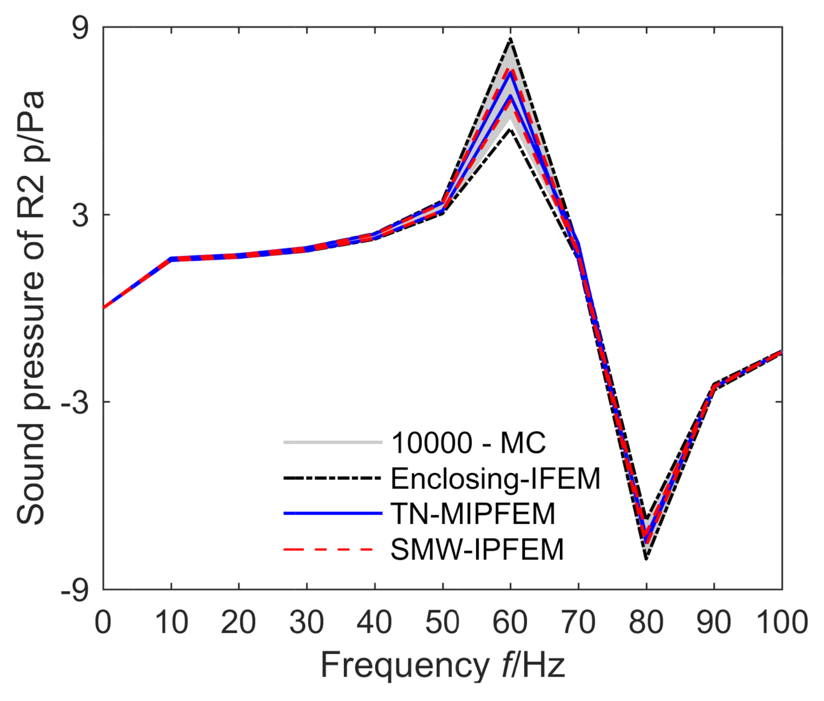
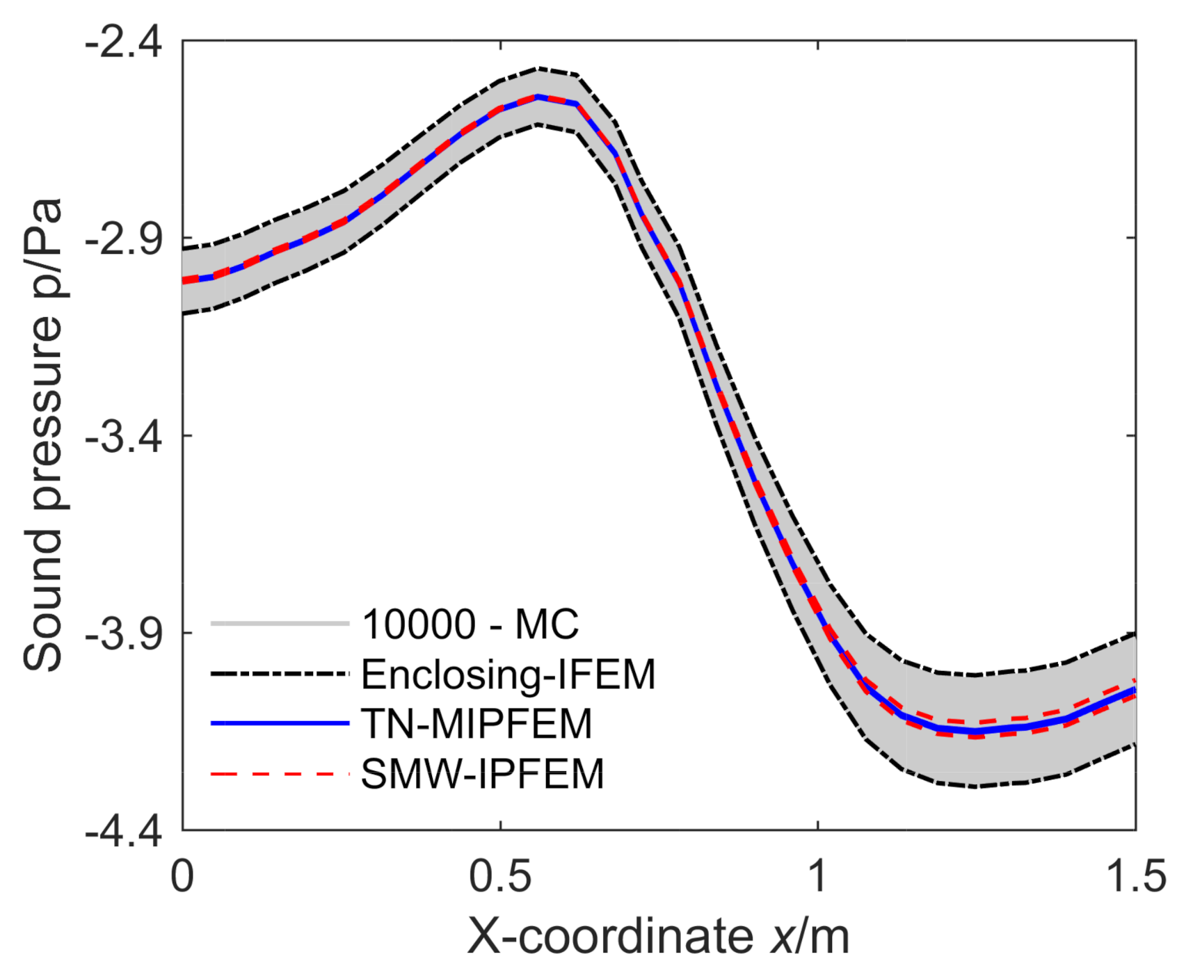
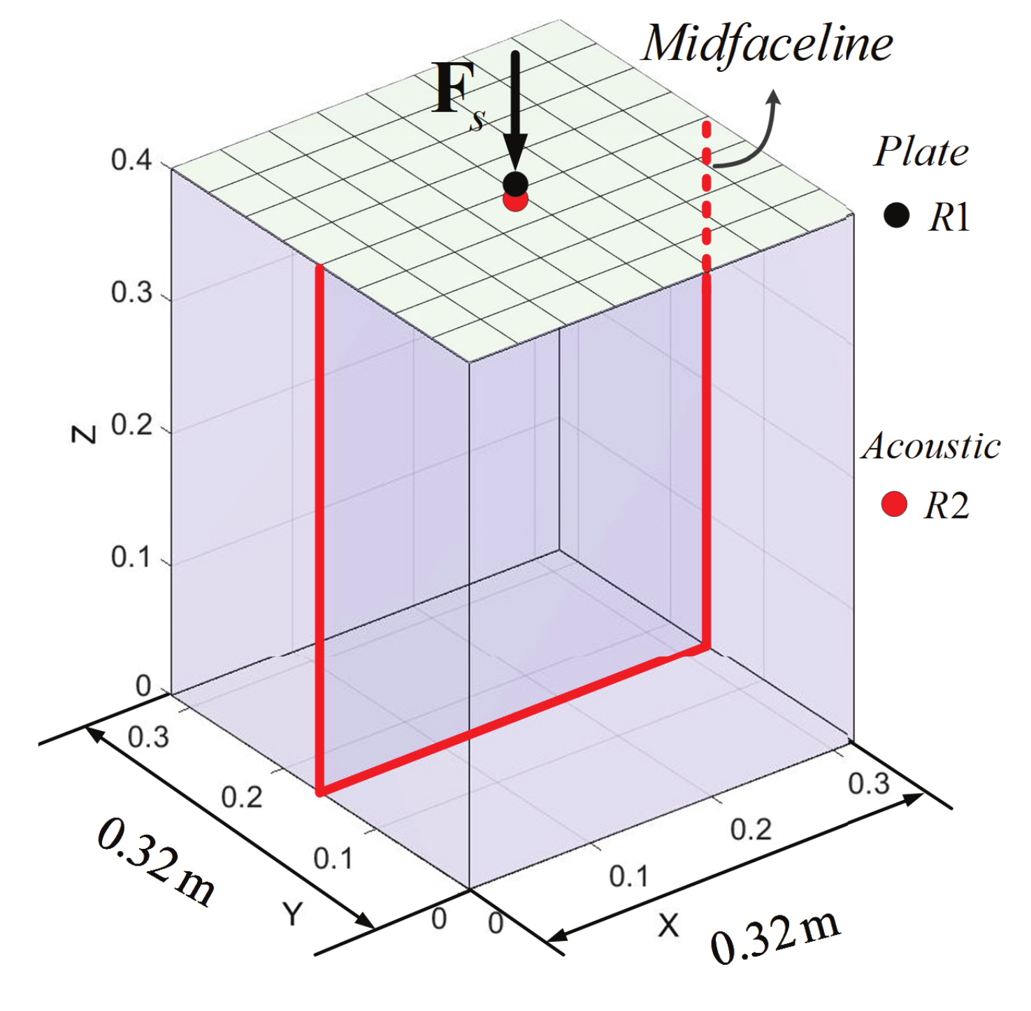
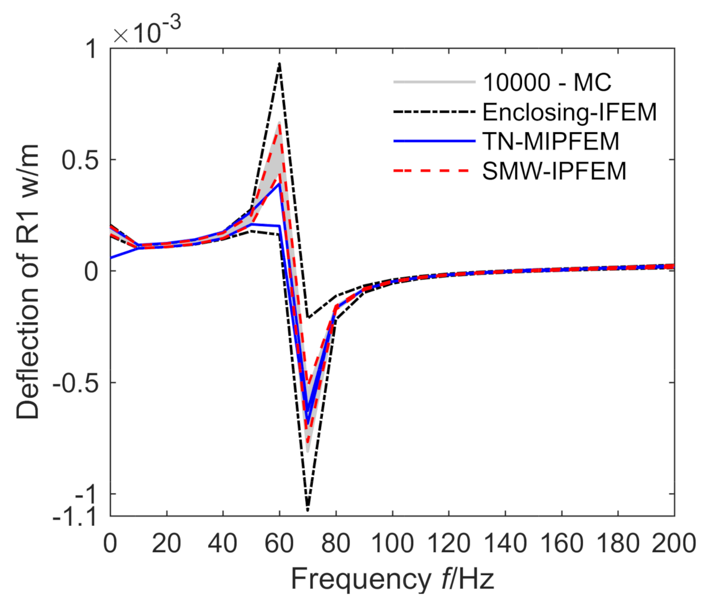
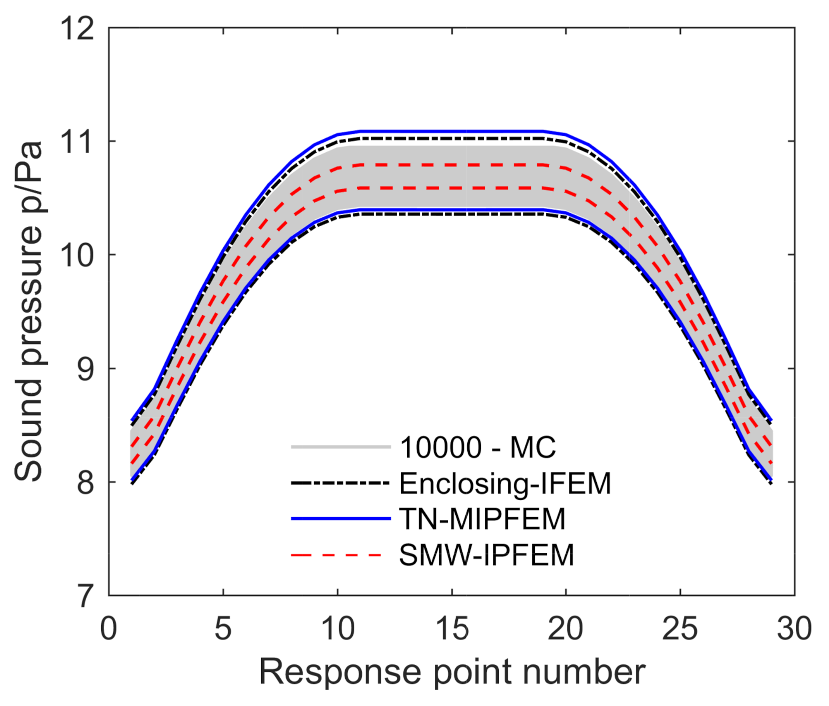
4.2. Numerical Analysis of a 3D Classical Vibro-Acoustic Coupling Model

The second application is focusing on the classical 3D vibro-acoustic coupling system with uncertain-but-bounded parameters, as this regular-shaped model has been examined by other suitable interval coupling analysis methods [24,25]. Figure 11 depicts a 3D Mindlin plate vibro-acoustic coupling model: the rectangular plate is located at the top of the cavity, and all edges are supposed to be simple support. The flexible plate is made of aluminum, with material parameters being $E=71\mathrm{Gpa},{\rho }_s=2700\mathrm{kg}/{\mathrm{m}}^3,\mu =0.3$, and the thickness of plate is $t=0.001\mathrm{m}$. The cuboid cavity is filled with air with a density of ${\rho }_f=1.21\mathrm{kg}/{\mathrm{m}}^3$ and sound speed of $c=343\mathrm{m}/\mathrm{s}$. The other boundary of acoustic cavity is presumed to be rigid, and the external load of the vibro-acoustic system is located on the central point of the plate by a unit force in the norm direction. In total, for the MITC4-element mesh of the plate, the number of elements and nodes are 64 and 81, while for the acoustic mesh with 8-nodes element, the numbers are 640 and 891, respectively. With the same estimation of uncertain level $\mathbf{\alpha }=0.025$ to structural parameters, the Young’s modulus E and the thickness of plate can be regarded as the interval variables

$$\begin{array}{c}\hfill \begin{array}{cc}& E^I=E^c+[-\mathbf{\alpha },\mathbf{\alpha }]\times E^c\hfill \\ & t^I=t^c+[-\mathbf{\alpha },\mathbf{\alpha }]\times t^c\hfill \end{array}\end{array}$$

(39)

Based on the previously mentioned IFEMs and Monte Carlo simulation with 10,000 samples, both of the frequency response at fixed response points and deterministic frequency response in the fixed locations are analyzed, and plotted in Figure 12, Figure 13 and Figure 14, respectively. Unlike other research, the fixed receiving points R1 and R2 are represented for the plate and acoustic differently, though these two nodes share the same coordinate. As such, it may be reasonable to obtain the results with significant difference. The analytical frequency band is from 0 to $200\mathrm{Hz}$ by the interval of $10\mathrm{Hz}$; both the upper and lower bounds of the solutions by different IFEMs will be described in the these figures, together with the large amount of Monte Carlo solution sets, that are represented with gray lines.

From Figure 12 and Figure 13, we can find that the reference solution by Monte Carlo method is included in the result by enclosing-IFEM; although the overestimation is happened in the resonant frequency, the conservativeness of the whole frequency band is fine compared with other perturbation-based methods. Another highlight is that the performance of the extension of SMW-IPFEM is better than the TN-MIPFEM, not only for the aspects of conservativeness, but also to the general trends of prediction. It means that the unimodal components’ decomposition turns to be a better choice in the process of tracing uncertainties. Nevertheless, in Figure 14, the conclusion is opposite, that the conservativeness of SMW-IPFEM is worse than the TN-MIPFEM, due to the unpredictable and non-conservative effect in SMW series approximation. Apparently, regardless of cases, the enclosing-IFEM still achieves the best trade-off in prediction, particularly in Figure 14 for the response of a single frequency, which is away from the resonant frequency $f=70\mathrm{Hz}$.

In

Table 2. The total calculation time by 10,000 MC, TN-MIPFEM, SMW-IPFEM, and enclosing-IFEM for 3D classical vibro-acoustic coupling model.

MC	TN-MIPFEM		SMW-IPFEM		Enclosing-IFEM
${\mathrm{T}}_{\mathrm{MC}}$	${\mathrm{T}}_1$	${\mathrm{T}}_1/{\mathrm{T}}_{\mathrm{MC}}$	${\mathrm{T}}_2$	${\mathrm{T}}_2/{\mathrm{T}}_{\mathrm{MC}}$	${\mathrm{T}}_3$	${\mathrm{T}}_3/{\mathrm{T}}_{\mathrm{MC}}$
4855.6 s	16.5 s	$3.4\times {10}^{-3}$	1422.8 s	$2.9\times {10}^{-1}$	35.8 s	$7.3\times {10}^{-3}$

, it is clear to see that the IFEMs is more efficient than the traditional probabilistic methods, especially compared to the TN-IPFEM and the new proposed enclosing-IFEM. As the increasing sizes for dyadic product shown in Equation (27), it spends more time for the SMW-IPFEM to calculate the approximate results.

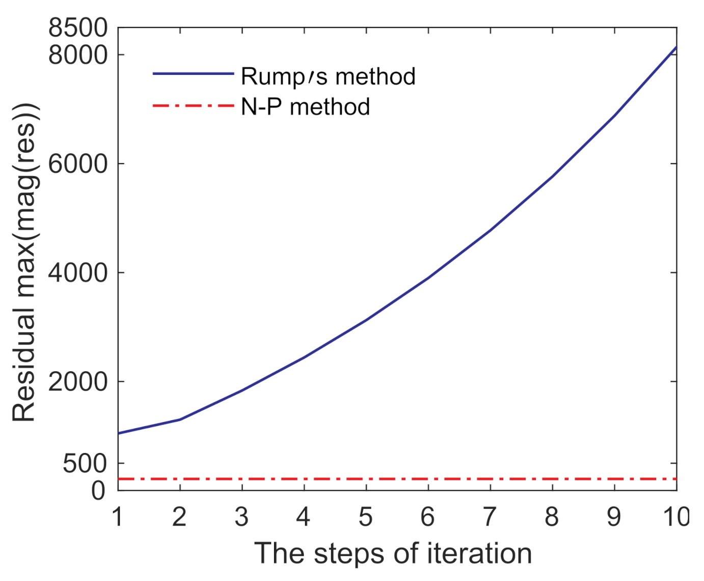
4.3. Convergence of Residual between Two Iterative Methods

The last concern for the proposed enclosing-IFEM is the residual of convergence, as the final solution of enclosing-IFEM is computed by iteration rather than other directed inversion or approximation. Most iterative methods terminate when the residual is sufficiently small, and the bad convergence of residual will result in overestimation in enclosing-IFEM. In order to tackle the overly-wide results in enclosing-IFEM, it is important to measure the residual convergence between the existing two iterative algorithms such that the former 3D classical coupling model is examined in both the conservativeness of bounds and the convergence of residual.

Figure 15 and Figure 16 depict the frequency response of receiving points R1 and R2, located in plate and acoustic field, respectively. With the same steps of iteration, it is clear to find that the bounds by the Neumaier–Pownuk iteration are more accurate than those by Rump’s algorithm. The reason is given in Figure 17, as it depicts that, after each step of iterative loop, the residual of the uncertain vibro-acoustic coupling system can be derived from the Equation (40), specified as

$$\begin{array}{c}\hfill Residual\left(n\right)=max\left(mag\left(res\left({\mathbf{x}}^n\right)\right)\right) =max\left(mag\left({\mathbf{b}}^I-\mathbf{A}{\mathbf{x}}^n\right)\right)\end{array}$$

(40)

As a result, the residual of Rump’s iteration is divergent, and the residual by Neumaier–Pownuk algorithm is much smaller than the Rump’s one. Hence, it cannot guarantee the accuracy of output solution by Rump’s theorem in coupling problems. Additionally, whereas the convergence is fast, the calculation time of Neumaier–Pownuk is also dominant compared with the other one.

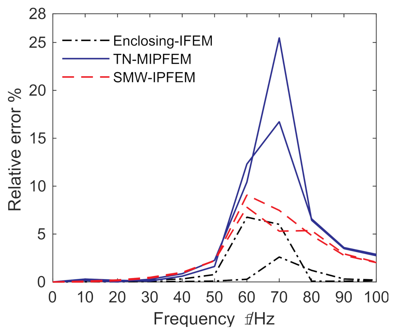
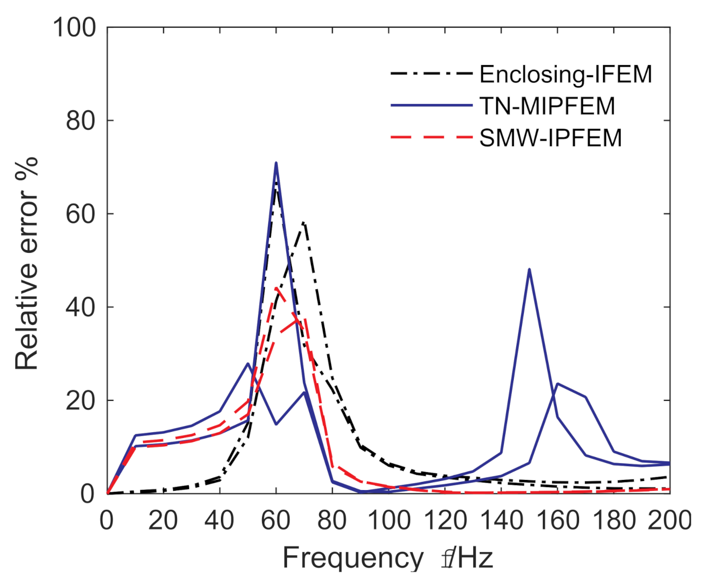
4.4. Analysis of the Relative Error

As Figure 8, Figure 9 and Figure 10 and Figure 12, Figure 13 and Figure 14 depict, although the conservativeness of solution sets can be guaranteed by the enclosing-IFEM, the error analysis needs to be introduced for evaluating the fluctuated effect of response [34]. By taking the Monte Carlo results as the reference of exact solution, the relative error of interval solutions of different IFEMs can be further expressed as the following formulas:

$$\begin{array}{c}\hfill \mathrm{Relative}\mathrm{error}=\left\{\begin{array}{c}\underline{Er}=\frac{\left|{\underline{\mathbf{p}}}_{IFEMs}-min\left({\mathbf{p}}_{MC}\right)\right|}{min\left({\mathbf{p}}_{MC}\right)}\times 100\%\hfill \\ \overline{Er}=\frac{\left|{\overline{\mathbf{p}}}_{IFEMs}-max\left({\mathbf{p}}_{MC}\right)\right|}{max\left({\mathbf{p}}_{MC}\right)}\times 100\%\hfill \end{array}\right.\end{array}$$

(41)

From Figure 18, the relative error of the proposed enclosing-IFEM is much smaller than others in 2D vibro-acoustic system with parametric uncertainties, while in Figure 19, it seems slightly larger than the solution by the SMW-IPFEM. However, from the single frequency response shown in Figure 20, the average relative error of enclosing-IFEM is still lower than the one by the SMW-IPFEM. To sum up, the relative error of the enclosing-IFEM maintains a reasonably low level compared with other IFEMs.

5. Conclusions

This research mainly proposed a new enclosing-IFEM for the applications of vibro-acoustic coupling problems with uncertain-but-bounded parameters. By introducing the technique of unimodal components’ decomposition and mixed-nodal-element (MNE) assemblage, the enclosing-IFEM based on the modified interval arithmetic strategy (MIAS) can be applied to the special case of uncertain vibro-acoustic problem (no damping and structural uncertainties). Comparative research on the perturbation-based methods and modified interval arithmetic strategy is objectively to provide some evaluation criterion for the numerical result analysis. From the numerical applications on 2D and 3D coupling cases, both of the validity and computational efficiency of the enclosing-IFEM are examined in the comparative studies, which include the Monte Carlo simulation, TN-MIPFEM, and SMW-IPFEM. Apparently, for the advantages of modified interval arithmetic strategy (MIAS), the upper and lower bounds of the solution sets by the enclosing-IFEM are more rational and conservative than other interval perturbation finite-element methods. Although the computational efficiency of the enclosing-IFEM is a little less than the TN-IPFEM from Table 1 and Table 2, the enclosing-IFEM is superior to SMW-IPFEM in calculation speed. With the better convergent iterative procedure (Neumaier–Pownuk method), we can reveal that the enclosing-IFEM achieves the best performance in both conservative bounds and computational efficiency. However, in engineering application, two difficulties hinder the application of the enclosing-IFEM; one is the high consumption of memory for iteration, the other is the inherent property of invasion in programming the enclosing-IFEM, which limits the application in present FE commercial software.

References

1. Atalla, N.; Sgard, F. Finite Element and Boundary Methods in Structural Acoustics and Vibration; CRC Press: Boca Raton, FL, USA, 2015. [Google Scholar]
2. Chen, Q.; Fei, Q.; Wu, S.; Li, Y. Uncertainty propagation of the energy flow in vibro-acoustic system with fuzzy parameters. Aerosp. Sci. Technol. 2019, 94, 105367. [Google Scholar]
3. Faes, M.; Moens, D. Recent trends in the modeling and quantification of non-probabilistic uncertainty. Arch. Comput. Methods Eng. 2020, 27, 633–671. [Google Scholar] [CrossRef]
4. Wang, L.; Liu, Y.; Liu, Y. An inverse method for distributed dynamic load identification of structures with interval uncertainties. Adv. Eng. Softw. 2019, 131, 77–89. [Google Scholar]
5. Wang, L.; Liu, J.; Yang, C.; Wu, D. A novel interval dynamic reliability computation approach for the risk evaluation of vibration active control systems based on PID controllers. Appl. Math. Model. 2021, 92, 422–446. [Google Scholar]
6. Moens, D.; Hanss, M. Non-probabilistic finite element analysis for parametric uncertainty treatment in applied mechanics: Recent advances. Finite Elem. Anal. Des. 2011, 47, 4–16. [Google Scholar]
7. Dessombz, O.; Thouverez, F.; Laîné, J.P.; Jézéquel, L. Analysis of mechanical systems using interval computations applied to finite element methods. J. Sound Vib. 2001, 239, 949–968. [Google Scholar]
8. Xia, B.; Yu, D. Interval analysis of acoustic field with uncertain-but-bounded parameters. Comput. Struct. 2012, 112, 235–244. [Google Scholar] [CrossRef]
9. Xia, B.; Yu, D.; Liu, J. Interval and subinterval perturbation methods for a structural-acoustic system with interval parameters. J. Fluids Struct. 2013, 38, 146–163. [Google Scholar] [CrossRef]
10. Moore, R.E. Interval Analysis; Prentice-Hall: Englewood Cliffs, NJ, USA, 1966; Volume 4. [Google Scholar]
11. Muhanna, R.L.; Mullen, R.L. Uncertainty in mechanics problems—Interval–based approach. J. Eng. Mech. 2001, 127, 557–566. [Google Scholar]
12. Fuchs, M. Unimodal formulation of the analysis and design problems for framed structures. Comput. Struct. 1997, 63, 739–747. [Google Scholar] [CrossRef]
13. Impollonia, N. A method to derive approximate explicit solutions for structural mechanics problems. Int. J. Solids Struct. 2006, 43, 7082–7098. [Google Scholar] [CrossRef] [Green Version]
14. Neumaier, A.; Pownuk, A. Linear systems with large uncertainties, with applications to truss structures. Reliab. Comput. 2007, 13, 149–172. [Google Scholar] [CrossRef]
15. Yaowen, Y.; Zhenhan, C.; Yu, L. Interval analysis of frequency response functions of structures with uncertain parameters. Mech. Res. Commun. 2013, 47, 24–31. [Google Scholar] [CrossRef]
16. Xiang, Y.; Shi, Z. Interval Analysis of Interior Acoustic Field with Element-By-Element-Based Interval Finite-Element Method. J. Eng. Mech. 2021, 147, 04021085. [Google Scholar] [CrossRef]
17. Chen, Q.; Fei, Q.; Wu, S.; Li, Y. Statistical energy analysis for the vibro-acoustic system with interval parameters. J. Aircr. 2019, 56, 1869–1879. [Google Scholar] [CrossRef]
18. Dong, J.; Ma, F.; Hao, Y.; Gu, C. An interval statistical energy method for high-frequency analysis of uncertain structural–acoustic coupling systems. Eng. Optim. 2020, 52, 2100–2124. [Google Scholar] [CrossRef]
19. Baklouti, A.; Dammak, K.; El Hami, A. Uncertainty Analysis Based on Kriging Meta-Model for Acoustic-Structural Problems. Appl. Sci. 2022, 12, 1503. [Google Scholar] [CrossRef]
20. Qiu, Z.; Chen, S.; Elishakoff, I. Bounds of eigenvalues for structures with an interval description of uncertain-but-non-random parameters. Chaos Solitons Fractals 1996, 7, 425–434. [Google Scholar] [CrossRef]
21. Xia, B.; Yu, D. Modified sub-interval perturbation finite element method for 2D acoustic field prediction with large uncertain-but-bounded parameters. J. Sound Vib. 2012, 331, 3774–3790. [Google Scholar] [CrossRef]
22. Xia, B.; Yu, D. Modified interval perturbation finite element method for a structural-acoustic system with interval parameters. J. Appl. Mech. 2013, 80, 041027. [Google Scholar] [CrossRef]
23. Wang, C.; Qiu, Z.; Wang, X.; Wu, D. Interval finite element analysis and reliability-based optimization of coupled structural-acoustic system with uncertain parameters. Finite Elem. Anal. Des. 2014, 91, 108–114. [Google Scholar] [CrossRef]
24. Wu, F.; Gong, M.; Ji, J.; Peng, G.; Yao, L.; Li, Y.; Zeng, W. Interval and subinterval perturbation finite element-boundary element method for low-frequency uncertain analysis of structural-acoustic systems. J. Sound Vib. 2019, 462, 114939. [Google Scholar] [CrossRef]
25. Wu, F.; Gong, M.; Yao, L.; Hu, M.; Jie, J. High precision interval analysis of the frequency response of structural-acoustic systems with uncertain-but-bounded parameters. Eng. Anal. Bound. Elem. 2020, 119, 190–202. [Google Scholar] [CrossRef]
26. Xu, M.; Du, J.; Wang, C.; Li, Y. A dimension-wise analysis method for the structural-acoustic system with interval parameters. J. Sound Vib. 2017, 394, 418–433. [Google Scholar] [CrossRef]
27. Xu, M.; Du, J.; Wang, C.; Li, Y. Hybrid uncertainty propagation in structural-acoustic systems based on the polynomial chaos expansion and dimension-wise analysis. Comput. Methods Appl. Mech. Eng. 2017, 320, 198–217. [Google Scholar] [CrossRef]
28. Xu, M.; Du, J.; Wang, C.; Li, Y.; Chen, J. A dual-layer dimension-wise fuzzy finite element method (DwFFEM) for the structural-acoustic analysis with epistemic uncertainties. Mech. Syst. Signal Process. 2019, 128, 617–635. [Google Scholar] [CrossRef]
29. Chen, N.; Xia, S.; Yu, D.; Liu, J.; Beer, M. Hybrid interval and random analysis for structural-acoustic systems including periodical composites and multi-scale bounded hybrid uncertain parameters. Mech. Syst. Signal Process. 2019, 115, 524–544. [Google Scholar] [CrossRef]
30. Impollonia, N.; Muscolino, G. Interval analysis of structures with uncertain-but-bounded axial stiffness. Comput. Methods Appl. Mech. Eng. 2011, 200, 1945–1962. [Google Scholar] [CrossRef]
31. Sandberg, G.; Wernberg, P.A.; Davidsson, P. Fundamentals of fluid-structure interaction. In Computational Aspects of Structural Acoustics and Vibration; Springer: Berlin/Heidelberg, Germany, 2008; pp. 23–101. [Google Scholar]
32. Desmet, W.; Vandepitte, D. Finite element modeling for acoustics. In ISAAC13-International Seminar on Applied Acoustics; Citesee: Leuven, Belgium, 2005; pp. 37–85. [Google Scholar]
33. Chen, S.H.; Wu, J. Interval optimization of dynamic response for structures with interval parameters. Comput. Struct. 2004, 82, 1–11. [Google Scholar] [CrossRef]
34. Chen, N.; Yu, D.; Xia, B.; Liu, J.; Ma, Z. Homogenization-based interval analysis for structural-acoustic problem involving periodical composites and multi-scale uncertain-but-bounded parameters. J. Acoust. Soc. Am. 2017, 141, 2768–2778. [Google Scholar] [CrossRef]
35. Köylüoğlu, H.U.; Çakmak, Ş.A.; Nielsen, S.R. Interval algebra to deal with pattern loading and structural uncertainties. J. Eng. Mech. 1995, 121, 1149–1157. [Google Scholar] [CrossRef]
36. Xiao, N.; Muhanna, R.L.; Fedele, F.; Mullen, R.L. Interval finite element analysis of structural dynamic problems. SAE Int. J. Mater. Manuf. 2015, 8, 382–389. [Google Scholar] [CrossRef]
37. Katili, I.; Batoz, J.L.; Maknun, I.J.; Lardeur, P. A comparative formulation of DKMQ, DSQ and MITC4 quadrilateral plate elements with new numerical results based on s-norm tests. Comput. Struct. 2018, 204, 48–64. [Google Scholar] [CrossRef]
38. Xiao, N. Interval Finite Element Approach for Inverse Problems under Uncertainty. Ph.D. Thesis, Georgia Institute of Technology, Atlanta, GA, USA, 2015. [Google Scholar]
39. Popova, E.D. Rank one interval enclosure of the parametric united solution set. BIT Numer. Math. 2019, 59, 503–521. [Google Scholar] [CrossRef]
40. Rump, S.M. INTLAB—Interval laboratory. In Developments in Reliable Computing; Springer: Berlin/Heidelberg, Germany, 1999; pp. 77–104. [Google Scholar]
Figure 1. The interior vibro-acoustic coupling system.
Applsci 12 03061 g001
Figure 2. The failure reason for EBE-IFEM to analyze the vibro-acoustic coupling problem.
Applsci 12 03061 g002
Figure 3. The assembly method for the mixed-nodal-element assemblage.
Applsci 12 03061 g003
Figure 4. Relationship between three different IPFEMs.
Applsci 12 03061 g004
Figure 5. Flow chart of Rump’s inclusion method.
Applsci 12 03061 g005
Figure 6. Flow chart of Neumaier–Pownuk method.
Applsci 12 03061 g006
Figure 7. 2D interior-car vibro-acoustic model.
Applsci 12 03061 g007
Figure 8. The sound pressure at the point of R1.
Applsci 12 03061 g008
Figure 9. The sound pressure at the point of R2.
Applsci 12 03061 g009
Figure 10. The sound pressure along the bottom-line at frequency 90 Hz.
Applsci 12 03061 g010
Figure 11. 3D classical vibro-acoustic model.
Applsci 12 03061 g011
Figure 12. The sound pressure at the point of R1.
Applsci 12 03061 g012
Figure 13. The sound pressure at the point of R2.
Applsci 12 03061 g013
Figure 14. The sound pressure along the midfaceline at frequency 100 Hz.
Applsci 12 03061 g014
Figure 15. The conservativeness comparison of sound pressure at the point of R1 by Rump’s method and Neumaier–Pownuk method.
Applsci 12 03061 g015
Figure 16. The conservativeness comparison of sound pressure at the point of R2 by Rump’s method and Neumaier–Pownuk method.
Applsci 12 03061 g016
Figure 17. The comparison of the residual convergence by Rump’s method and Neumaier–Pownuk method.
Applsci 12 03061 g017
Figure 18. Comparison of the relative errors of different IFEMs for the 2D interior-car vibro-acoustic coupling model at the receiving point of R2.
Applsci 12 03061 g018
Figure 19. Comparison of the relative errors of different IFEMs for the 3D classical vibro-acoustic coupling model at the receiving point of R2.
Applsci 12 03061 g019
Figure 20. Comparison of the relative errors of different IFEMs for the 3D classical vibro-acoustic coupling model along the midface line at frequency 100 Hz.
Applsci 12 03061 g020