Abstract
Photovoltaic panels can be affected by partial shading, which causes some shaded cells to consume the energy generated by other cells of the panel. That is, shaded cells stop operating in the first quadrant and start operating in the second quadrant, with negative voltage at their terminals, causing power losses and other negative effects in the cells. The Bishop model is an accurate representation of the cells behavior at the second quadrant, but estimating its parameters is not a trivial task. Therefore, this paper presents a procedure to estimate the parameters of the Bishop model by using the Chu–Beasley optimization technique. The effectiveness of this procedure was evaluated using different accuracy measures such as RMSE and MAPE, obtaining values lower than 0.5%. In addition, the results of this study demonstrate that it is essential to estimate all the parameters of the Bishop model, illustrate the variation in the parameters according to the cell technology and show the strong influence of the shunt resistance into the behavior at the second quadrant.
1. Introduction
Photovoltaic (PV) cells are devices that convert solar irradiance into electricity. This type of energy source has three main advantages: (1) it has an estimated lifespan of 25 years, (2) it does not require short-term maintenance and (3) its raw material is renewable [1,2]. However, the energy production of a PV system depends on the weather conditions of the place where the system is installed, which can quickly change. The behavior of the PV cell under particular environmental conditions is often described by using the current–voltage (I–V) curve, because it provides relevant information about the transformed energy and it can be used to calculate the maximum power that can be delivered to a load [3]. The cell behavior for different irradiance and temperature conditions can be modeled using an equivalent electrical circuit, which is designed to represent the electrical phenomena associated with the energy transformation process [4,5,6,7].
The most commonly studied circuital models are the single-diode model (SDM) [8,9,10,11] and the double-diode model (DDM) [12,13,14,15]. Both have been used to model commercial PV cells, modules and panels made of monocrystalline silicon (mc-SI) or polycrystalline silicon (pc-SI). However, when a PV panel is under partial shading, the shaded PV cells might not generate energy; on the contrary, they might consume the energy produced by the other cells of the panel. In this phenomenon, known as reverse bias, the cell exhibits a negative voltage at its terminals; therefore, it operates in the second quadrant (negative voltage and positive current). It is worth noting that neither SDM or DDM can accurately represent this phenomenon at the cell level.
The previous condition has been addressed by using the avalanche mechanism to represent the reverse bias at the cell level. This is the case of the Bishop model [16,17], which introduces a variation to the SDM that affects the shunt resistance current () by means of an ohmic term and a non-linear multiplication factor. Such a model, proposed in [18], was implemented to analyze the database, which contains the I–V profiles of mc-SI cells. In particular, the parameters proposed in [18] correspond to the average value of the parameters obtained for each cell in the database; unfortunately, that study does not include a detailed description of the procedure used to estimate the model parameters. Other authors have used this Bishop model to analyze PV systems [19,20,21] because it estimates the cell behavior under partial shading conditions at the cell level. In general, the parameters suggested by Bishop are adopted when the second quadrant is analyzed [18].
A simulation method was developed in [19] to diagnose PV systems, where the PV current of the shaded region is calculated as a relationship between the current under standard operating conditions, the irradiance value and the applied shadow. Although that work does not emphasize the estimation of the parameters related to the first quadrant, the parameters associated with the second quadrant are selected equal to the values reported by Bishop in [18]. A more general approach was proposed in [21], where a method for modeling PV arrays and modules was based on calculating the I–V relationship regardless of whether the arrays or modules have different electrical connections. The general equations system was obtained by applying Kirchhoff’s laws and the damped Newton method was used for calculating the system solution. The PV system in that work was built in layers; the first one from cell to module and the second one from module to array. Nevertheless, that study does not specify the method adopted to estimate the model parameters. The Bishop model has also been used to develop tools (such as PVSIM) to evaluate the performance of PV cells, modules, arrays and large-scale PV systems [20]; for example, PVSIM also includes elements such as bypass diodes and blocking diodes. Concerning the model parameters, PVSIM incorporates information for different operating points (irradiance and temperature) to interpolate the parameters values for a particular temperature defined by the user. In addition, the user can define a set of parameters; thus, cell-level information should be obtained to estimate those parameters. However, that work does not describe the procedure adopted to find the parameters values incorporated into the tool database.
The parameters of a PV cell can be estimated by different approaches, where the most commonly adopted ones are analytical methods and stochastic techniques (such as heuristics and metaheuristics) [22,23,24,25,26], which are often called optimization techniques. Analytical methods are based on equations that relate the output current and voltage of the system and, despite those approaches determine the parameters of a PV model, those depend on variables under standard test conditions (STC). Thus, if those parameters are not adequately defined, analytical methods are unable to reproduce the variations in PV profiles due to changes in temperature and irradiance. Although these methods are simple, the resulting models have low performance in the reproduction of different real operating conditions [27,28,29].
The optimization techniques are classified in two important groups, the deterministic and the stochastic ones. For the deterministic ones, there are solution methods, such as Newton–Raphson [30], Gauss–Seidel [31] and other methods [32], which are related to methods that require a convex, continuous and differentiable expression of an equation or mathematical model; given this context, it is necessary to clarify that the convergence of an algorithm can stay within a local minimum due to the complexity and non-linearity of the Bishop model.
On the other hand, the stochastic methodology is divided into two groups, heuristics and metaheuristics. For the parametric estimation, the metaheuristics approach has been more notable; it contains a randomness factor. In this case, aspects related to the procedure for the selection of candidate solutions, setting parameters and objective function impact the reached solution; further, a statistical analysis is required to validate the results [25,33].
Optimization algorithms are also widely adopted to estimate the parameters that best fit an I–V profile of a PV cell, module, or panel. Those methods can be used to minimize the energy consumption and costs or maximize the profits, production, performance, or energy efficiency. One of the most used techniques for parameter estimation of the SDM is the genetic algorithm (GA). For example, in [34], a GA is used to analyze the behavior of the estimated parameters as irradiation and temperature changes. Similarly, in [35], a comparative analysis of the parameter estimation of the SDM is performed, evaluating the results provided by the Newton–Raphson algorithm against optimization techniques such as GA and particle swarm optimization (PSO). Besides, hybrid techniques which use analytical formulations and numerical algorithms have been proposed to improve computation time or accuracy. In [36], mathematical formulations to translate I–V curves and a moth-flame algorithm are used to take into account the PV cell parameters sensitivity to weather conditions on the SDM.
In short, optimization techniques can be applied in many PV applications as long as the equation to be optimized can be expressed in terms of an objective function, i.e., a mathematical model that can be used in an iterative process [25,37,38]. However, the use of optimization techniques require trade-offs between accuracy, computation time and computational resources, which are defined by the method programming and objective function. As it can be noticed in the literature review, optimization techniques have been widely used for estimating the parameters of cells or modules mostly using the SDM or the DDM, which do not represent the behavior of the cell in the second quadrant in a proper way. On the other hand, the Bishop model improves the representation of the cell behavior at the second quadrant, but eight parameters of an implicit model must be determined. However, to the best of the authors’ knowledge, procedures for estimating its parameters are not reported in the literature. Instead, most of the works concerning PV cell or array analysis based on Bishop model adopt the parameters from other studies previously reported. Therefore, the purpose of this paper is to propose a methodology to estimate the parameters of the Bishop mathematical model to represent a PV cell in both the first and second quadrants. Because the high number of parameters to be identified and the implicit and non-linear relationship between output current and voltage of Bishop model, an optimization approach based on a Chu–Beasley genetic algorithm was used. The estimation process is divided into two stages; in the first stage, the curve in the first quadrant is modeled based on the estimation of SDM parameters; then, using the first five calculated parameters, the Bishop parameters are estimated to reproduce the I–V curve in both the first and second quadrants. In the second stage, the behavior in the first and second quadrants is modeled entirely by the Bishop model. Both estimation stages are validated based on the I–V curves of two PV cells (that are constructed with different technologies) using the root mean square error (RMSE).
The rest of the paper is organized as follows: Section 2 presents the Bishop model using an equivalent circuit, describing the equation that relates the output current and voltage of a PV cell and defining the set of parameters to be estimated. In addition, Section 2 also defines the objective function and the search ranges for the parameters. Then, Section 3 describes the GA method implemented in this work to perform the proposed parameter estimation, which is based on the Bishop mathematical model. Section 4 presents the experimental analysis and reports the results of the parameter estimation process of two PV cells (one mc-SI and one pc-SI). Those results are analyzed with the average values and standard deviation of the parameters, the objective function value, the computation time and the evaluation of accuracy metrics, such as RMSE, MAPE and MBE. Moreover, that section also provides a summary of the proposed methodology. Finally, the last section discusses the most relevant findings of this study in the conclusions.
2. Bishop PV Model
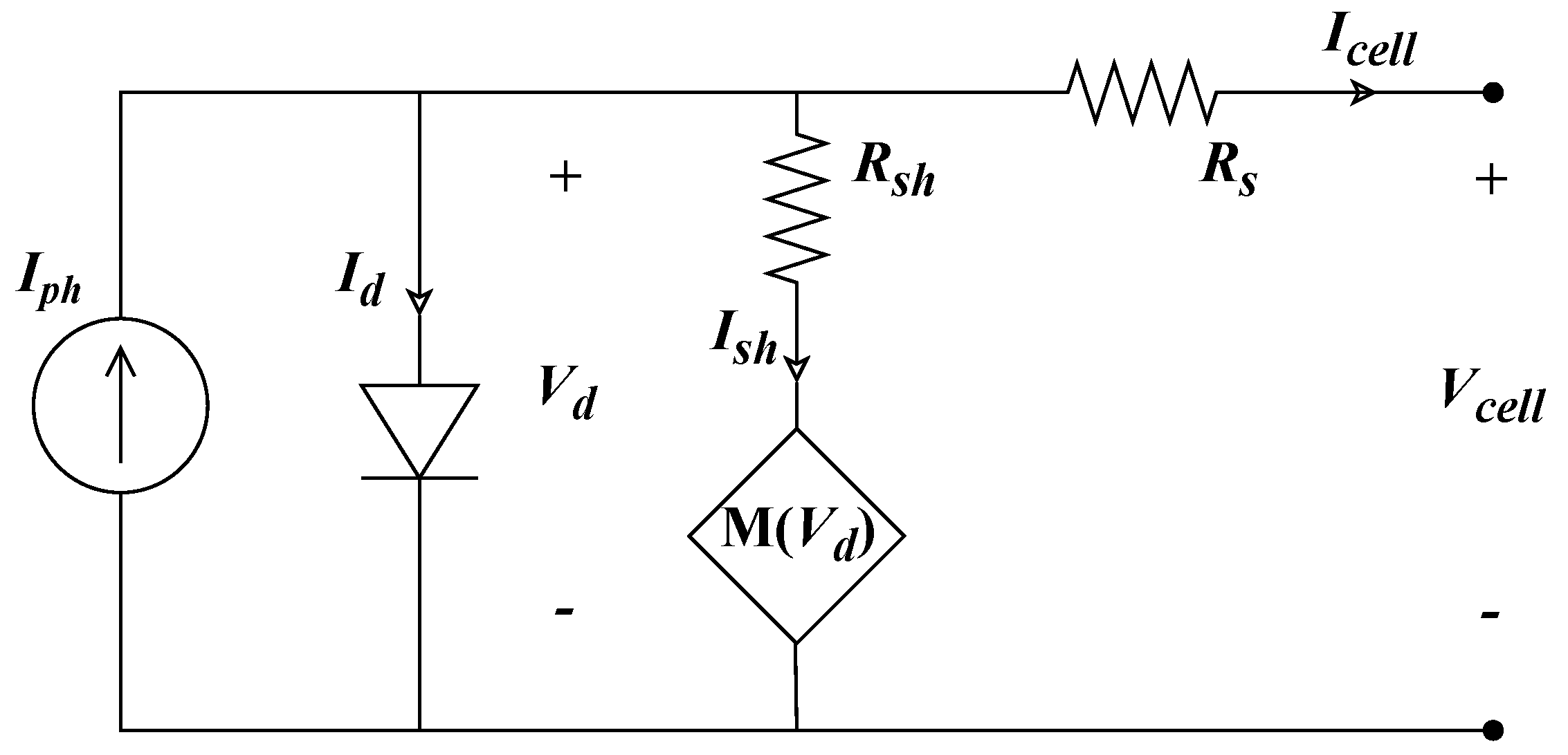
Figure 1 shows the circuital model of a PV cell proposed by Bishop [39]. It consists of a current source, associated with the generation of photovoltaic current (); a diode, representing the energy level threshold so that photons can trigger a significant production and circulation of electron–hole pairs across the junction; a series resistance (), representing losses due to contact resistance; and a shunt resistance (), representing leakage currents along the cell edges.

Figure 1.
The Bishop model of a photovoltaic cell.
To calculate the output current of the cell (), a summation of currents is performed as shown below in Equation (1).
The current–voltage relationship of the diode (, ) can be represented by the Shockley equation as given in Equation (2), where is the saturation current; is the ideality factor; k is the Boltzman constant; T is the cell temperature in kelvin degrees (K); and q is the electron charge.
Finally, the current through the shunt resistance () can be written as reported in Equation (3), where a is the fraction of the ohmic current related to the breakdown of the semiconductor; is the breakdown voltage; and m is the avalanche exponent.
The voltage across the diode can be expressed as follows:
In conclusion, eight model parameters should be estimated to reproduce the behavior of a PV cell using the Bishop model: , , , , , a, and m. Moreover, the relationship between the output current and the voltage at the cell terminals is implicit and non-linear; thus, it requires iterative techniques for its evaluation.
3. Mathematical Formulation of the Optimization Problem
The parameter estimation of the Bishop model was performed by means of a GA, which is a metaheuristic optimization technique. The optimization process was based on the objective function given in (5), which corresponds to the root mean square error (RMSE) between the current measured in the experimental tests () and the estimated value (). For this purpose, both data vectors should be taken from the same voltage vector and have the same size (n).
The constraints of the optimization problem correspond to the search ranges of the parameters to be estimated, which are defined in Equations (6)–(13). Those search ranges should be respected to ensure a correct estimation of the current using Equation (1).
Regarding the parameters associated with the SDM (, , , and ), it is possible to find defined ranges for different cell technologies in the literature. However, the parameters’ ranges that affect the second quadrant behavior (a, and m) have not been extensively studied; therefore, those ranges are described in Section 4.2.2.
3.1. Chu–Beasley Genetic Algorithm Applied to the Problem of Parameter Estimation
Equation (5) in Section 2 represents the problem addressed in this study and shows that iterative methods should be applied to find a solution. This study proposes two stages to solve said problem: (1) estimation of the SDM parameters and (2) estimation of Bishop parameters that can be used to represent the cell-level PV profiles in the first and second quadrants, where the GA is used to find the optimal parameter configuration. The following subsection describes the five fundamental steps of the GA.
3.1.1. Generation of the Initial Population
The first step is defining the coding of the estimation problem. In this case, each individual is represented as a row vector and each position in the vector represents each one of the parameters to be estimated.
The initial population is a matrix , where p is the number of individuals in the population and r is the number of parameters in the problem. The values of each position in the matrix (15) can be randomly generated, but they should fall within the search ranges defined in the set of constraints of the problem, as shown in the Equation (16), where is a random number. Therefore, the population is a different set each time the algorithm is executed. In this way, the neighborhood of the global minimum is reached taking different paths for each solution; those solutions could be different, but all of them exhibit an acceptable accuracy. In addition, the criterion of diversity should be satisfied, i.e., all individuals in the population should be different.
The objective function of each individual of the initial population must be evaluated. Then, the individual with the lowest objective function value (best solution found so far) is selected as the incumbent, because the goal is to obtain the lowest RMSE value between the estimated and the measured data.
3.1.2. Descendant Generation
In this iterative process, a child is produced in each generation as a result of three steps: (1) selection of individuals from the initial population, known as parents; (2) recombination of the information contained in the selected parents; (3) mutation of the combined information of the parents. These three steps are explained in detail below.
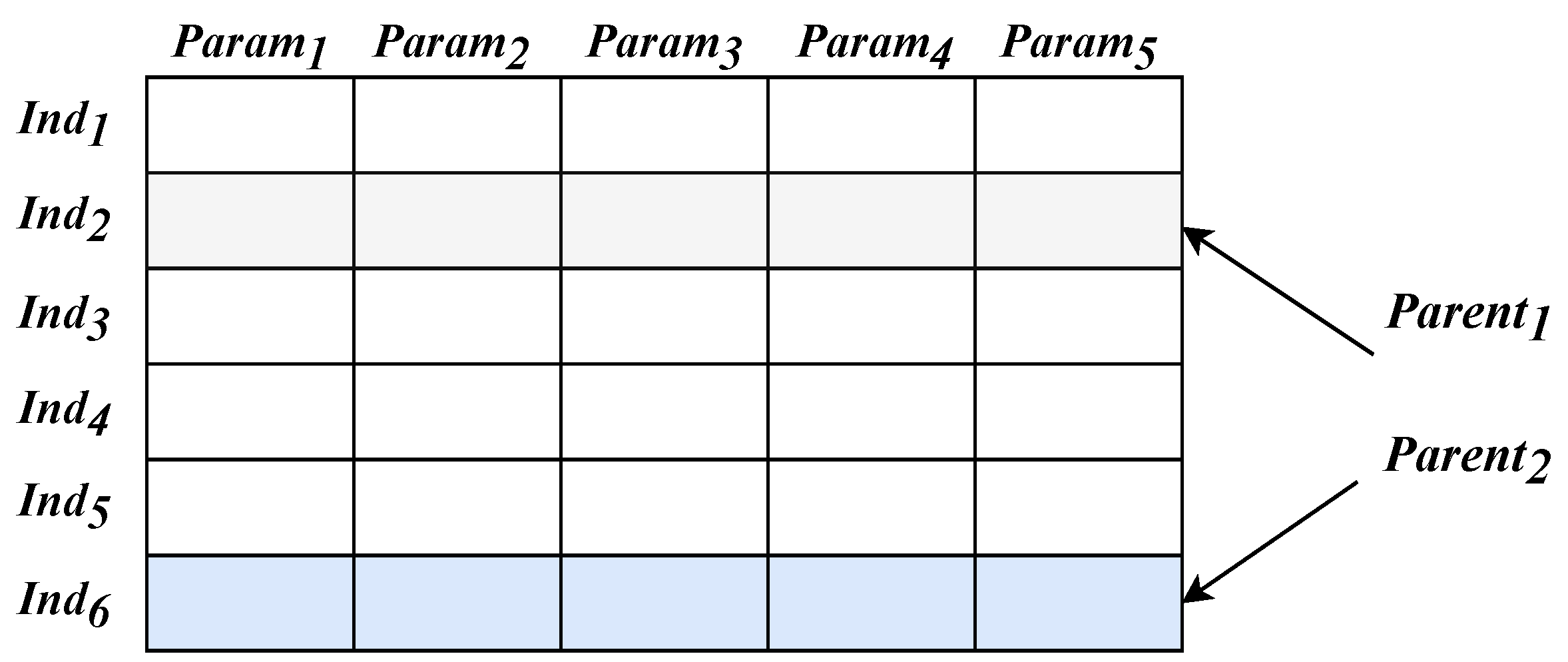
- Selection:Two parents are randomly selected from the initial population, where the two parents should be different individuals. In this work, the function from MATLAB was used, which returns a vector with two unique integers selected randomly from 1 to p. Figure 2 shows an example population with five parameters and six individuals, where Individuals 2 and 6 have been randomly selected as parents.
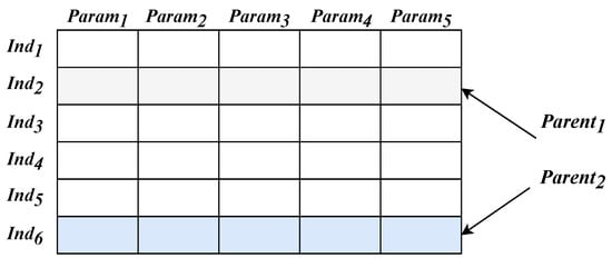 Figure 2. Selection process in the genetic algorithm.
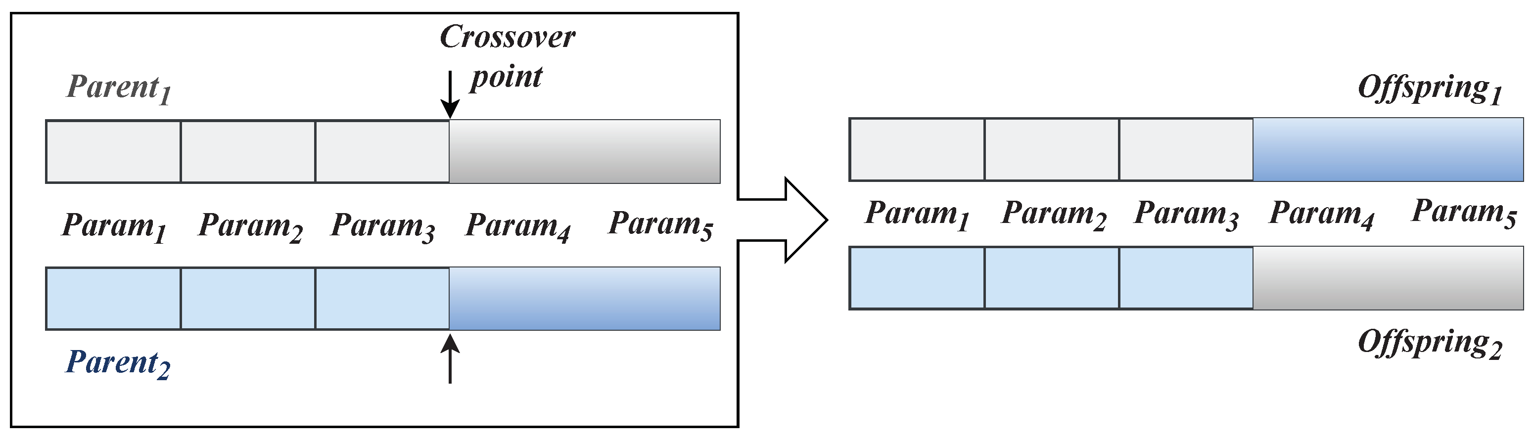
 - Crossover:At this step, information from both parents is combined to obtain descendants (offspring). For this purpose, a crossover point should be randomly selected in the vectors of the individuals selected as parents. The function from MATLAB allows users to generate a value, vector, or matrix with random integers uniformly distributed in a predefined interval; thus, it was used in this work to obtain the crossover point. In this case, since this work is intended for parameters with real values, the position of each one of the parameters should be respected because their search ranges are usually different. Figure 3 shows an example of recombination where Parameter 3 was selected as the crossover point.
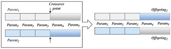 Figure 3. Crossover process in the genetic algorithm.
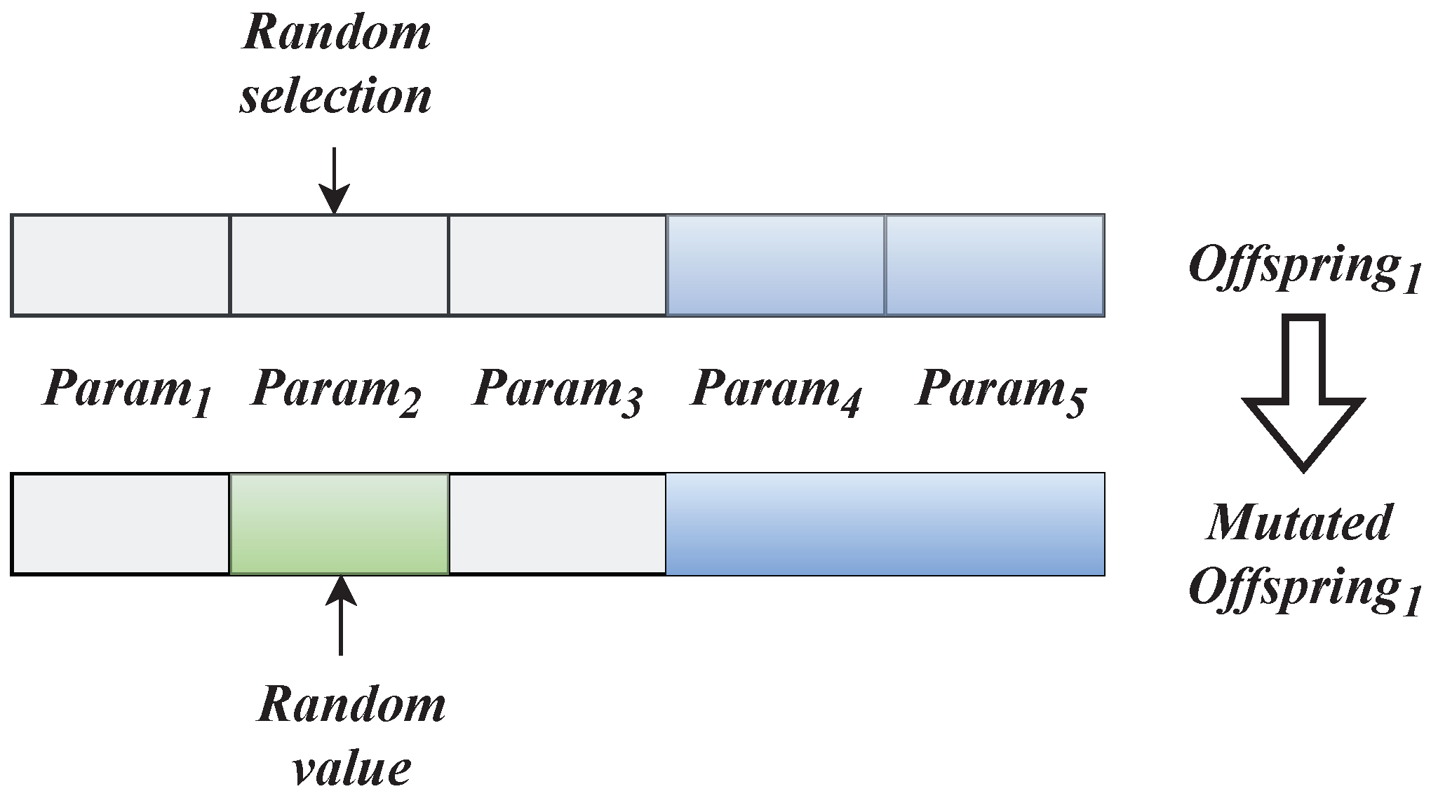
 - Mutation:At this step, variations are introduced in the offspring while preserving information inherited from their parents. Initially, it is decided whether or not both offspring will be mutated based on a randomized number that can take the values 0 or 1. If the value is 0, no mutation is performed; but, if it is 1, mutation takes place. If the decision is to mutate the offspring, the parameter to be mutated is randomly selected and replaced by a random value within its search range. Figure 4 shows this process.
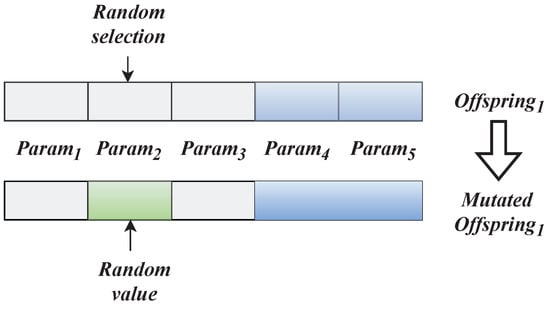 Figure 4. Mutation process in the genetic algorithm.
3.1.3. Offspring Selection
The descendant that continues the process is also randomly selected. Once it is selected, its objective function is evaluated.
3.1.4. Parent Update
The algorithm checks that the selected child is not part of the initial population (diversity criterion). If this condition is met, this descendant replaces the worst parent in the initial population. In addition, the algorithm checks whether this new individual has the best objective function in the entire population; if so, it replaces the incumbent.
3.1.5. Evaluation of the Stopping Criteria
This process has two stopping criteria: (1) maximum number of iterations to be evaluated in the estimation process () and (2) maximum number of consecutive iterations in which the incumbent is not improved ().
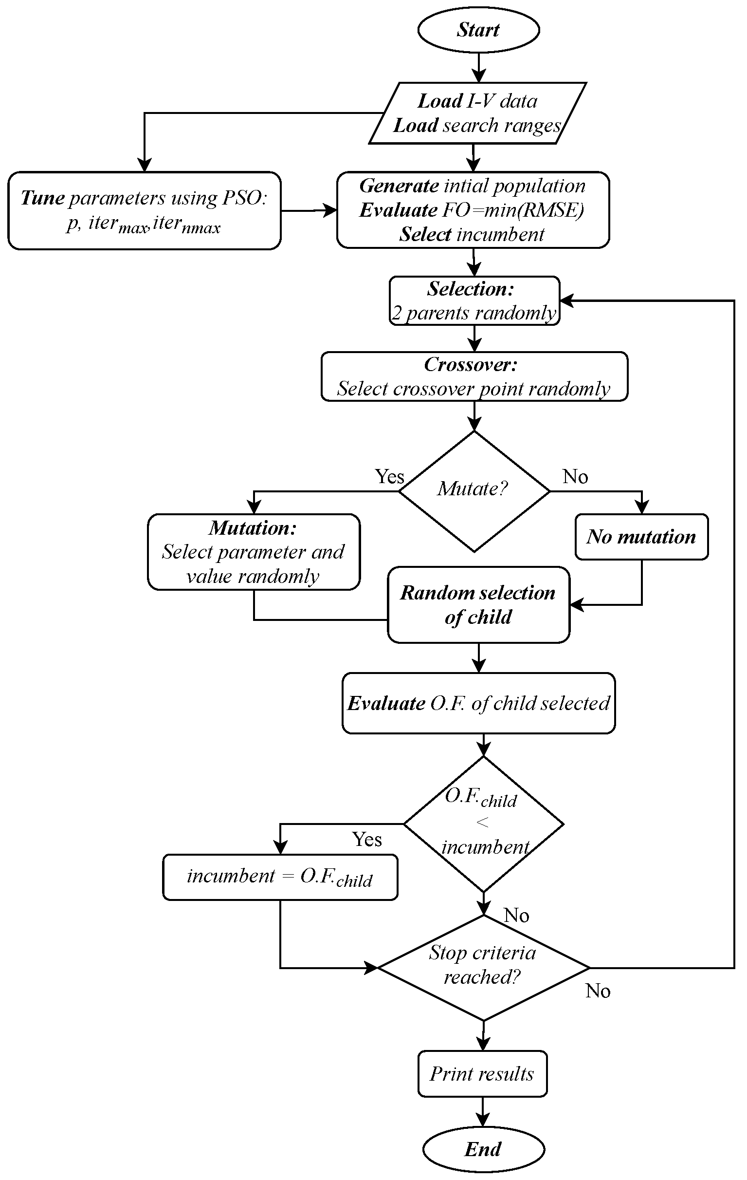
Finally, Algorithm 1 shows the pseudocode implementation of the GA used for the parameter estimation of the Bishop model. In addition, the flowchart of the proposed parameter estimation method is presented in Figure 5.
| Algorithm 1: Pseudocode proposed for the genetic algorithm. |
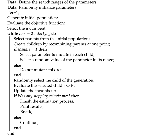 |

Figure 5.
Flowchart: PV estimation parameters using GA.
4. Results
4.1. Experimental Stage
The ERDM-SOLAR 10/12 panel was selected to validate the parameter estimation processes. Table 1 reports the most important data sheet parameters.

Table 1.
Datasheet parameters for ERDM-SOLAR 10/12 panel.
Additionally, to analyze the variation of the parameters of each panel technology, two panels of the same reference (one mc-SI and one pc-SI) were used. In each case, a cell with shaded area was selected to experimentally obtain its I–V curve in both the first and second quadrants. The procedure to obtain the curve at cell level is described as follows:
- The bypass diode included in the junction box of the PV panel was removed.
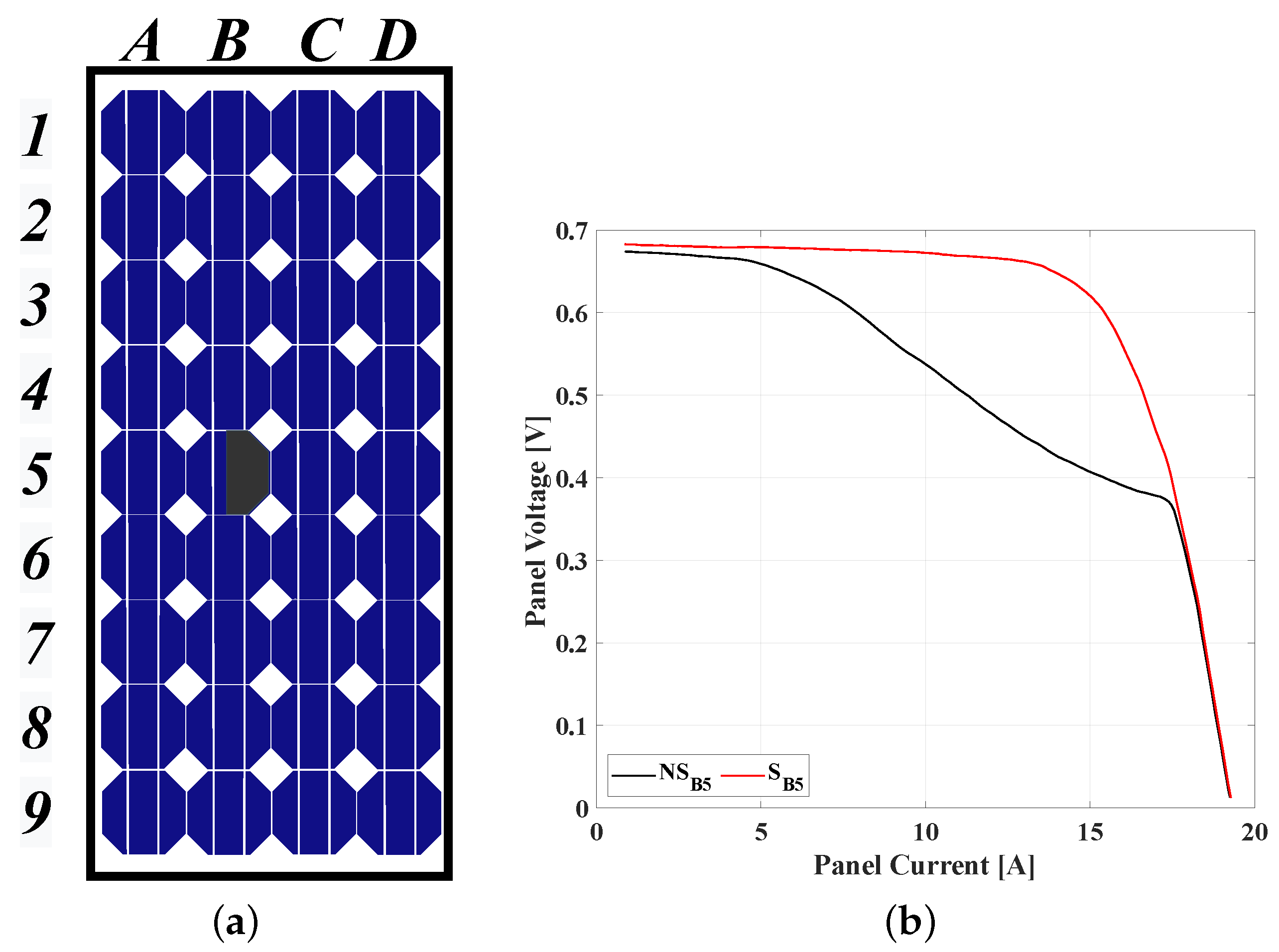
- Two I–V curves had to be obtained from the PV panel terminals; both were named with the corresponding location of the cell in the PV panel (see Figure 6a). The first one, curve, was taken without shading. The second curve was obtained by covering a percentage of the cell area, in this case corresponding to (); Figure 6b shows those curves. Both curves should be taken under similar irradiation and temperature conditions.
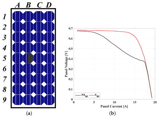 Figure 6. Case study example: (a) nomenclature of cells and location of ; (b) PV I–V curves with shaded and without shading.
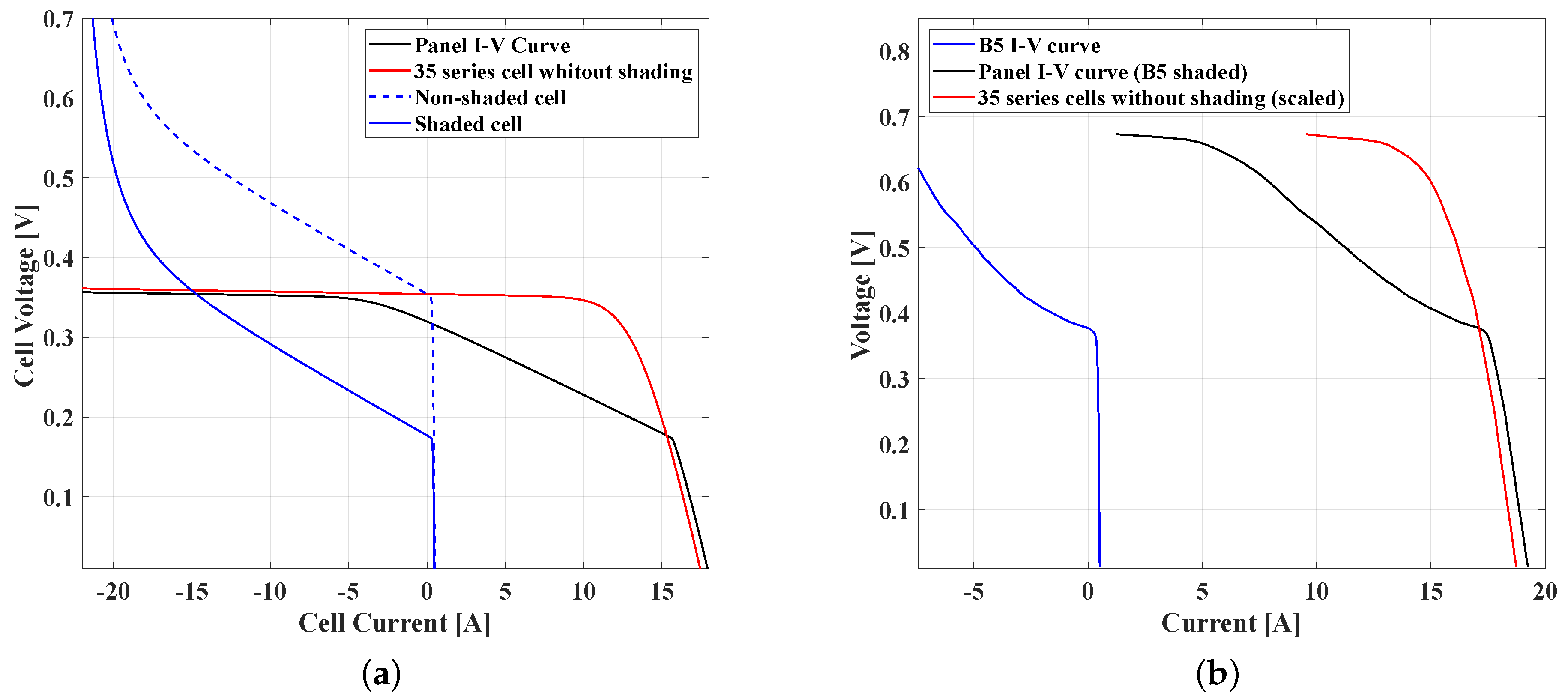
 - Figure 7a presents a 36-cell serial array, where a single cell is shaded. The behavior corresponding to the shaded cell is the blue curve, while the red curve represents the I–V curve of the remaining 35 cells. Given its series connection, the output current was the same through all cells, but the output voltage was the sum of the voltages of the 35 cells without shading and the voltage of the shaded cell for the other curve. In this way, the I–V curve of the shaded cell was reconstructed through the difference between the two I–V curves obtained, i.e., with and without shading. Later, it was necessary to scale the voltage of the curve without shading to match the 35 cells without shading of the other curve (the one with a single shaded cell), as follows: .
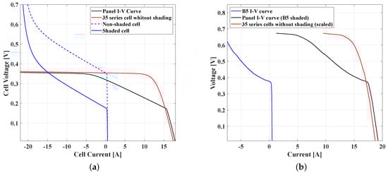 Figure 7. Graphical analysis for shading phenomena (a) from simulation and (b) from experimental analysis.
 - It was necessary to create a current vector with the highest value between the minimum currents of both curves as a minimum limit. The lowest value was chosen among the maximum currents of both curves as the upper limit. The current vector interpolated both curves (shaded I–V curve and unshaded scaled) to allow their subtraction to be performed, thus obtaining the current for the shaded cell. An example of this procedure is shown in Figure 7b, where the result of the experimental I–V curve of the shaded B5 cell is shown.
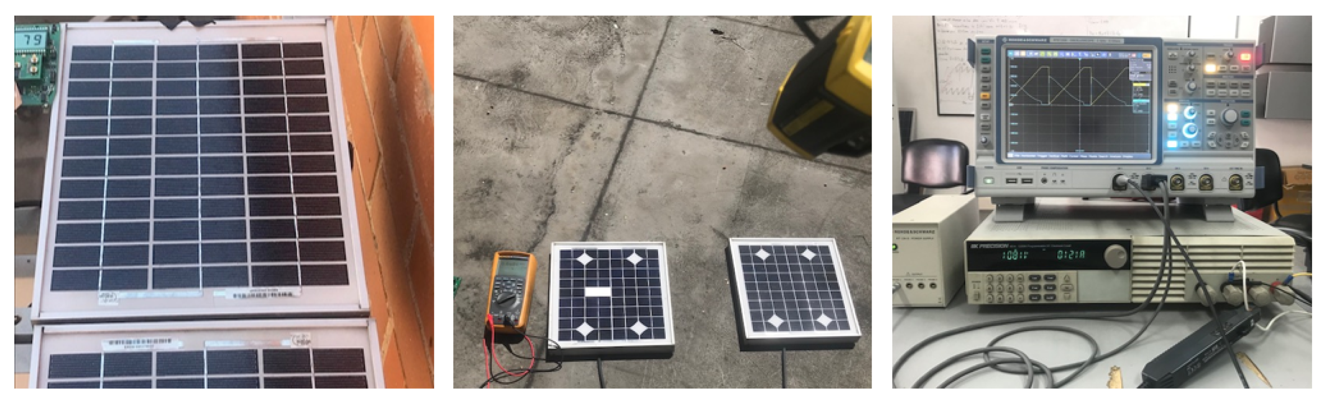
The experimental I–V data required in this process were obtained performing a programmed voltage sweep on an electronic load using the experimental setup shown in Figure 8, where an oscilloscope (right photo) recorded the current and voltage of the cell (left photo) and small PV modules were short-circuited (center photo) to estimate the irradiance value. Thus, the experimental I–V curves of both mc-SI and pc-SI cells were generated under real operating conditions, with an irradiance of 1008 W/m and a temperature of K; Figure 9 shows the experimental I–V curves. The R&S RTE1204 oscilloscope used in the experiments had an accuracy for DC measurements of [40]; hence, this precision must be propagated to the estimated values. Moreover, the short-circuit current was measured in another panel with the same characteristics to guarantee that the curves were obtained for similar irradiation. In this way, if the current did not change considerably, it can be assumed that the irradiation did not change either. This was also ensured by taking at least three curves for each experiment and, if there were differences among the three curves, the data were discarded and the experiment was performed again.

Figure 8.
Equipment used to obtain experimental I–V curves: ERDM-SOLAR 10/12 panel, reference panels and R&S RTE1204 oscilloscope.
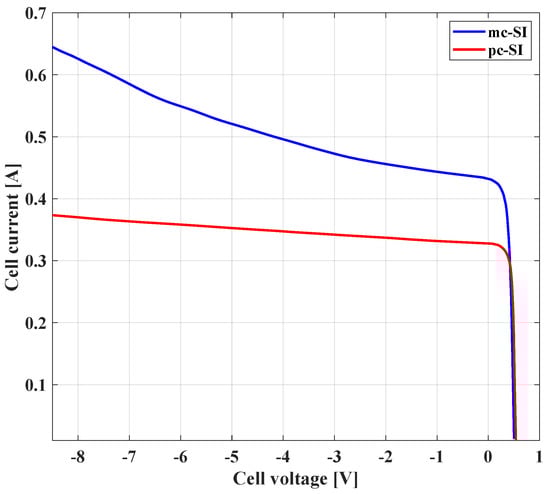
Figure 9.
Experimental I–V curves of mc-SI and pc-SI cells.
4.2. Estimation Stages
4.2.1. Estimation of the SDM Parameters
In the first stage of the parameter estimation, the five parameters defining the behavior of the curve in the first quadrant (, , , and ) were calculated. Thus, the ranges in Table 2 were selected as search ranges; those values were taken from the literature [41,42,43,44,45,46,47,48,49]. The photovoltaic current () was adjusted to a range of of the short-circuit current of the test (), this based on the fact that is caused by the generation and collection of light-generated carriers; therefore, and are very close values.
Table 2.
Ranges for the estimation of parameters in the first quadrant.
The genetic algorithm was adjusted to obtain the best possible solution in terms of the objective function. This was achieved by implementing another optimization algorithm to obtain the GA parameters that best fit the minimization of the problem. In this case, we used the PSO algorithm proposed in [50,51] to tune the following values: population size p (individuals or particles), with a search range of 2–100; number of iterations (maximum iterations allowed in the GA), with a search range of 1–10,000; and number of non-improvement iterations (this determines the point at which the algorithm stops performing convergence or minimizing the objective function), with a search range of 1–10,000. The results obtained from this tuning process were , and .
As part of the estimation process, the technique was evaluated 100 times per cell to observe metrics such as mean value and standard deviation for each estimated SDM parameter, which are reported in Table 3. The accuracy of the data was evaluated using the RMSE, since that metric was adopted as the objective function, obtaining small standard deviations for both cells, as reported in Table 4. The MAPE metric also showed a small error but with a higher standard deviation, especially for Cell 2, while the MBE metric exhibited very small values with high standard deviations. In any case, the three metrics had small values, which ensured a high accuracy on the I–V curves reproduction.
Table 3.
Ranges of parameters estimated for the SDM model (mean ± standard deviation).
Table 4.
Accuracy measures for estimation with the SDM model (mean ± standard deviation).
Analyzing the Cell 1 (mc-SI) parameters in Table 3, the highest relative deviations was found in , with . Concerning Cell 2 (pc-SI), the highest relative deviations were found in parameters and , with and , respectively. Instead, the other parameters, for both cells, exhibited variations under . The mean RMSE of Cell 1, evaluated as the objective function, was lower than the value obtained for Cell 2; however, the relative deviations for Cell 2 were lower than in the case of Cell 1.
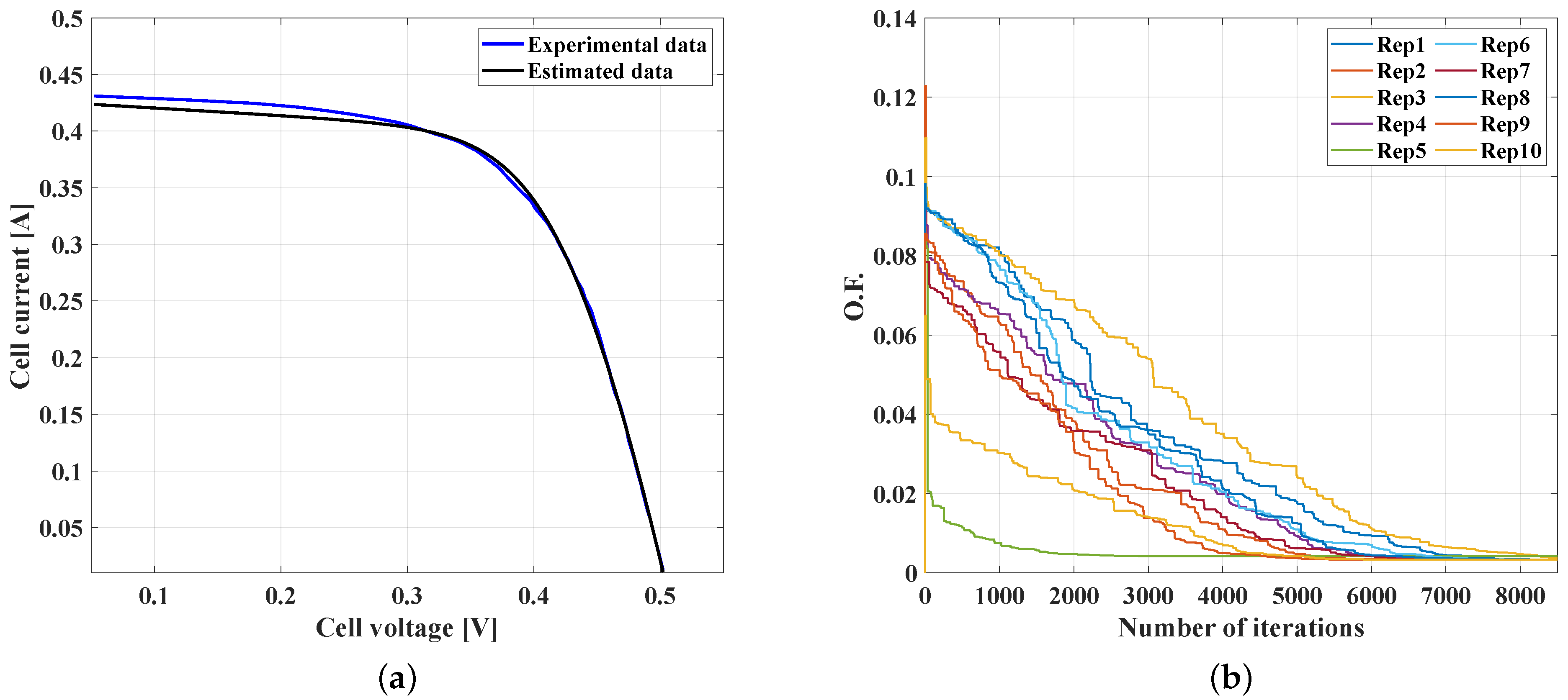
The best and worst solutions provided by the 100 estimations were also analyzed and compared based on the value of the objective function provided by the GA. Table 5 presents the sets of parameters that provide the best and worst performance for the SDM in each cell. Moreover, Figure 10a and Figure 11a show the comparison between the I–V curves estimated with the best parameters and the experimental data for Cells 1 and 2, respectively. Those figures show a satisfactory reproduction of the I–V curve’s first quadrant using the SDM parameters obtained with the proposed GA, where the most significant differences are presented in and . In addition, Figure 10b and Figure 11b show the convergence path of a sample of 10 repetitions of the estimation algorithm. Both figures show that the algorithm started with different initial values but arrived at similar objective function (O.F.) values, which resulted in parameters with low deviations.
Table 5.
Sets of parameters of the best and worst solutions for the SDM of each PV cell.
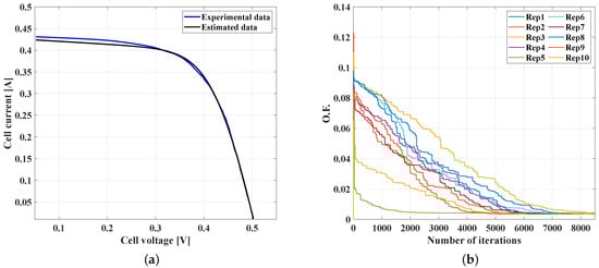
Figure 10.
Parameter estimation results for Cell 1 (mc-SI) using the SDM model: (a) comparison of I–V curves using the best solution and (b) convergence results for a sample of 10 repetitions.
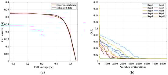
Figure 11.
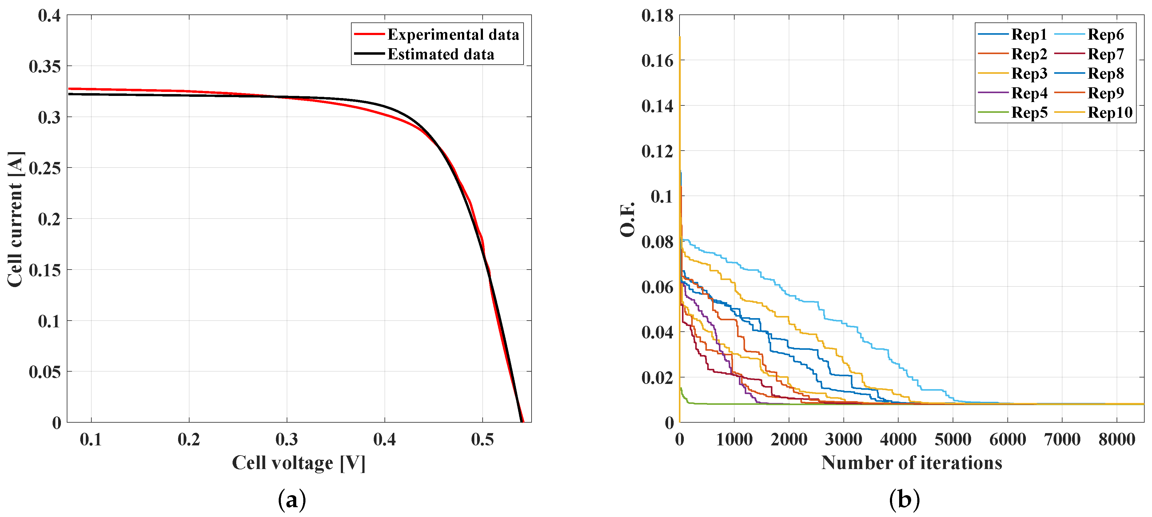
Parameter estimation results for Cell 2 (pc-SI) using the SDM mode: (a) comparison of I–V curves using the best solution and (b) convergence results for a sample of 10 repetitions.
In order to reproduce the I–V curve second quadrant, an exhaustive search in the literature was conducted to find Bishop model parameters used for PV cells, modules, or panels. Such a literature review confirmed that second-quadrant studies are commonly performed using parameters similar to those proposed in [18], with small variations; moreover, only few studies have reported the procedure followed to obtain those parameters. Table 6 lists some of the second-quadrant studies found in the literature, the values adopted for the second-quadrant parameters, the technology of the cell under study and the source from where the parameters were taken.
Table 6.
Values of the Bishop model parameters for the second quadrant.
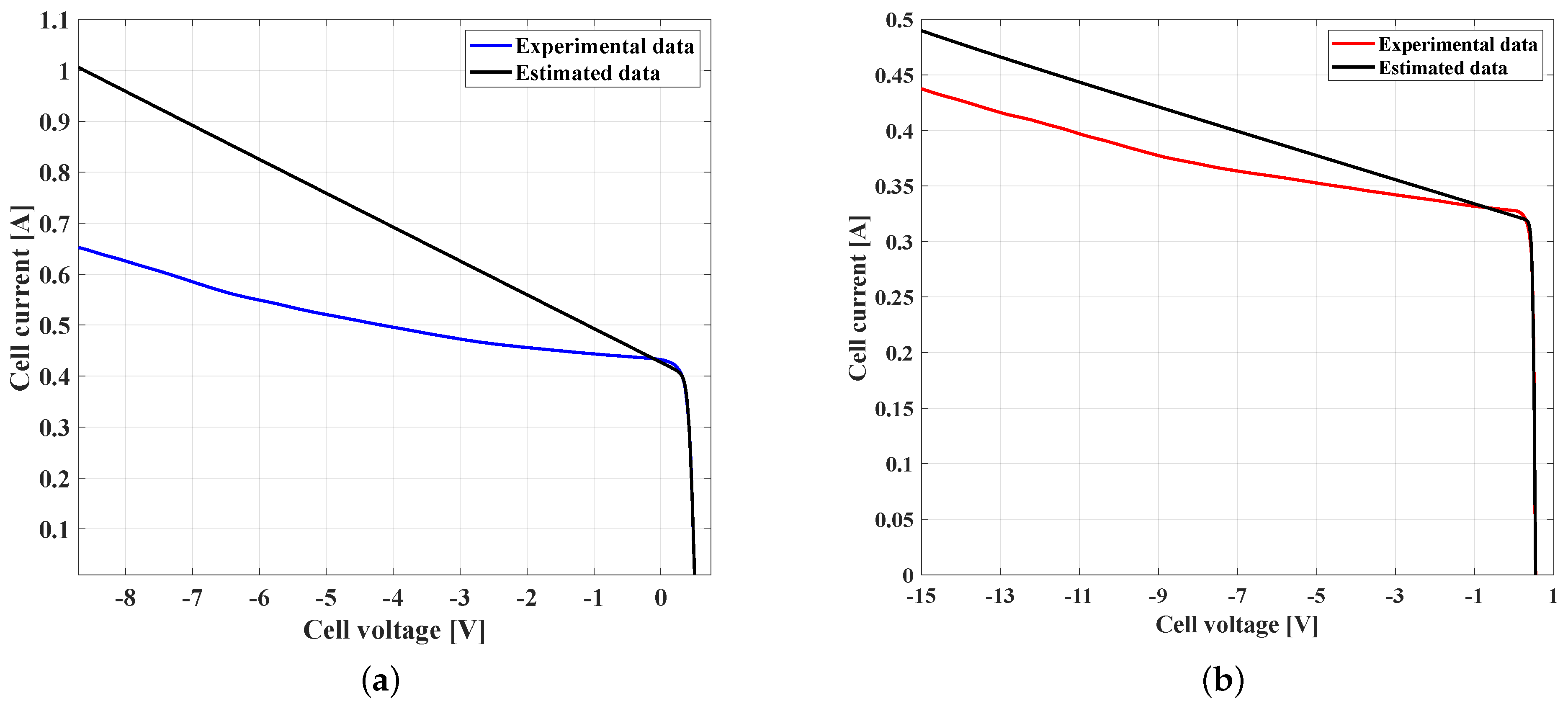
The values most commonly adopted in the literature for the second-quadrant parameters, observed in Table 6, are: , and V for Cell 1 and V for Cell 2. Using those values to estimate the behavior of both experimental cells (Cell 1 and Cell 2) led us to the results reported in Figure 12a,b, which shows a wrong reproduction of the second-quadrant behavior of real PV cells under real operation conditions. In fact, the RMSE of Cells 1 and 2 were and , respectively, which are much higher than the RMSE obtained in the first quadrant. Table 7 reports the RMSE, MAPE and MBE metrics for those curve reproductions, where all the metrics grow consistently in comparison with the values achieved in Table 4 for the parameter estimation of the SDM model. Therefore, this test puts into evidence the need to also estimate the second-quadrant parameters instead of adopting the values reported in [18] for any condition. The following subsection addresses such a second estimation stage.
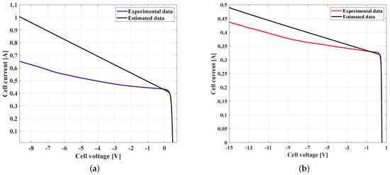
Figure 12.
Comparison of I–V curves using the Bishop model with the parameters of the SDM estimation and (a) Cell 1 (mc-SI) , , V; (b) Cell 2 (pc-SI) , , V.
Table 7.
Accuracy measures for estimation with the SDM model and Bishop parameters (mean ± standard deviation).
Finally, Figure 12a,b shows that, although the Bishop model is used to represent the behavior of PV cells, its fitting is not consistent in the second quadrant if the parameters are not correct. In fact, as the negative voltage increases, the difference between the estimated and experimental curves grows noticeable. The main reason of such an error increment is the fact that the estimation includes only information from the first quadrant to find the parameters from the SDM.
4.2.2. Estimation of the Bishop Model Parameters
This second estimation stage was carried out for the two cells with different technologies previously described (Cell 1 and Cell 2) to observe variations in the second quadrant parameters. In this case, in addition to the search ranges defined in Table 2, the ranges of parameters a, and m were also defined. Those additional ranges were obtained by analyzing the impact of each parameter on the I–V curve in the second quadrant. This procedure was carried out using simulations, verifying the values of which allowed us to reconstruct the I–V curve close to the experimental ranges obtained from the real cells. Those new parameter ranges are detailed in Table 8.
Table 8.
Ranges for parameter estimation in the second quadrant.
The objective function was the same adopted in the previous stage, i.e., Equation (5); the set of constraints indicated in Equations (6)–(13) also held, which are detailed in Table 2 and Table 8. As in the previous stage, the PSO algorithm was used to find the best set of parameters of the GA, similar to the tuning process presented in Section 4.2.1. In this case, the results were , and . Then, using those GA parameters, the estimation of the Bishop model was repeated 100 times, obtaining the parameters’ mean and standard deviations reported in Table 9. Moreover, Table 10 presents the sets of parameters providing the best and worst estimations obtained with the 100 repetitions.
Table 9.
Parameters estimated for the Bishop model (mean ± standard deviation).
Table 10.
Best and worst parameter solutions for the Bishop model of each PV cell.
In this estimation process, the highest relative deviations were found in the same parameters: , , m and a. For Cell 1, those maximum variations were , , and , respectively, while, for Cell 2, those were , , and , respectively; the other parameters reported variations under . The mean RMSE for Cell 1 (mc-SI), evaluated as the objective function, was lower than the value of Cell 2; however, the deviations were higher in Cell 2 (pc-SI).
Table 11 reports the accuracy metrics evaluated for the complete Bishop model estimation. Comparing the results presented in Table 7 and Table 11 confirm the large accuracy increment achieved with this second estimation stage, in comparison with the adoption of classical Bishop parameters found in the literature. In fact, the RMSE, MAPE and MBE values were reduced between one and two orders or magnitude.
Table 11.
Accuracy measures for estimation with the Bishop parameters (mean ± standard deviation).
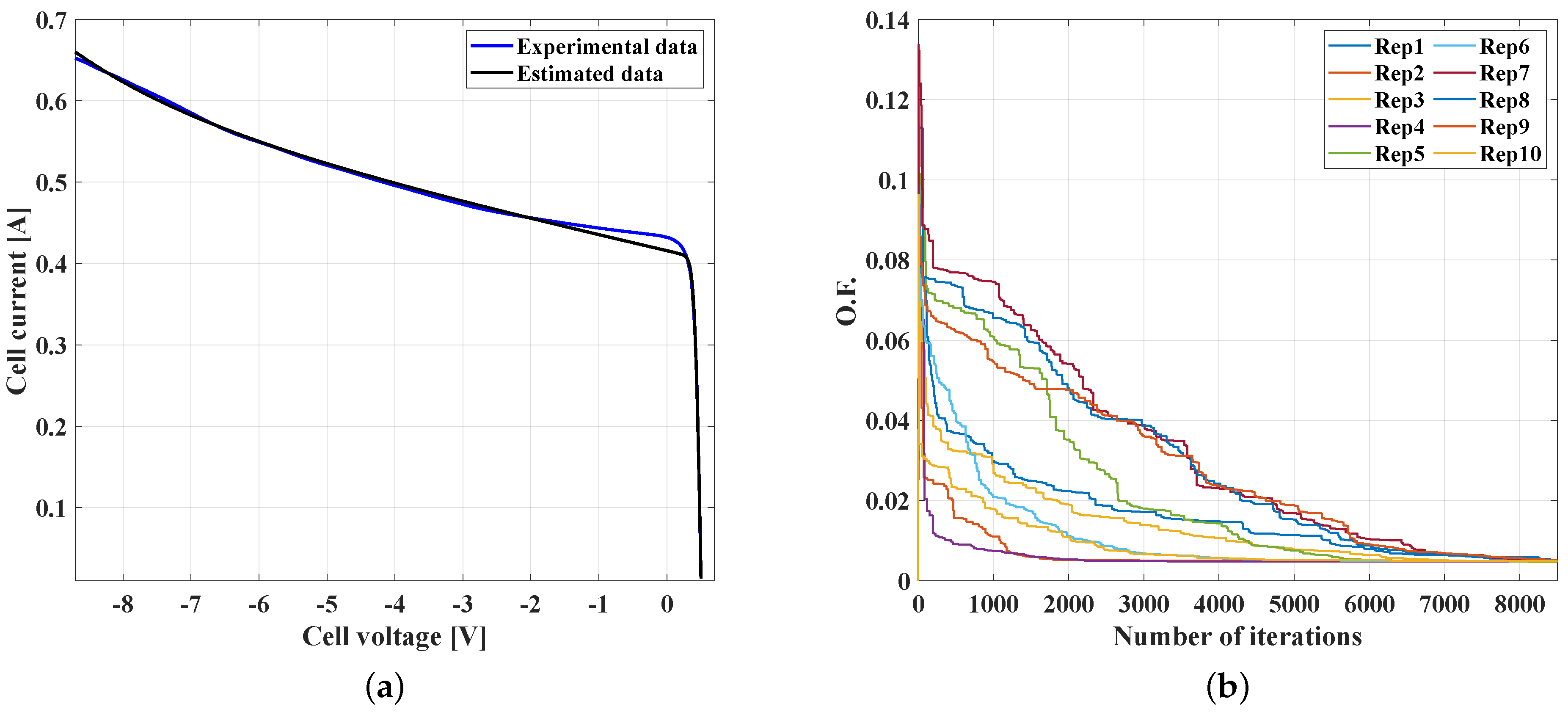
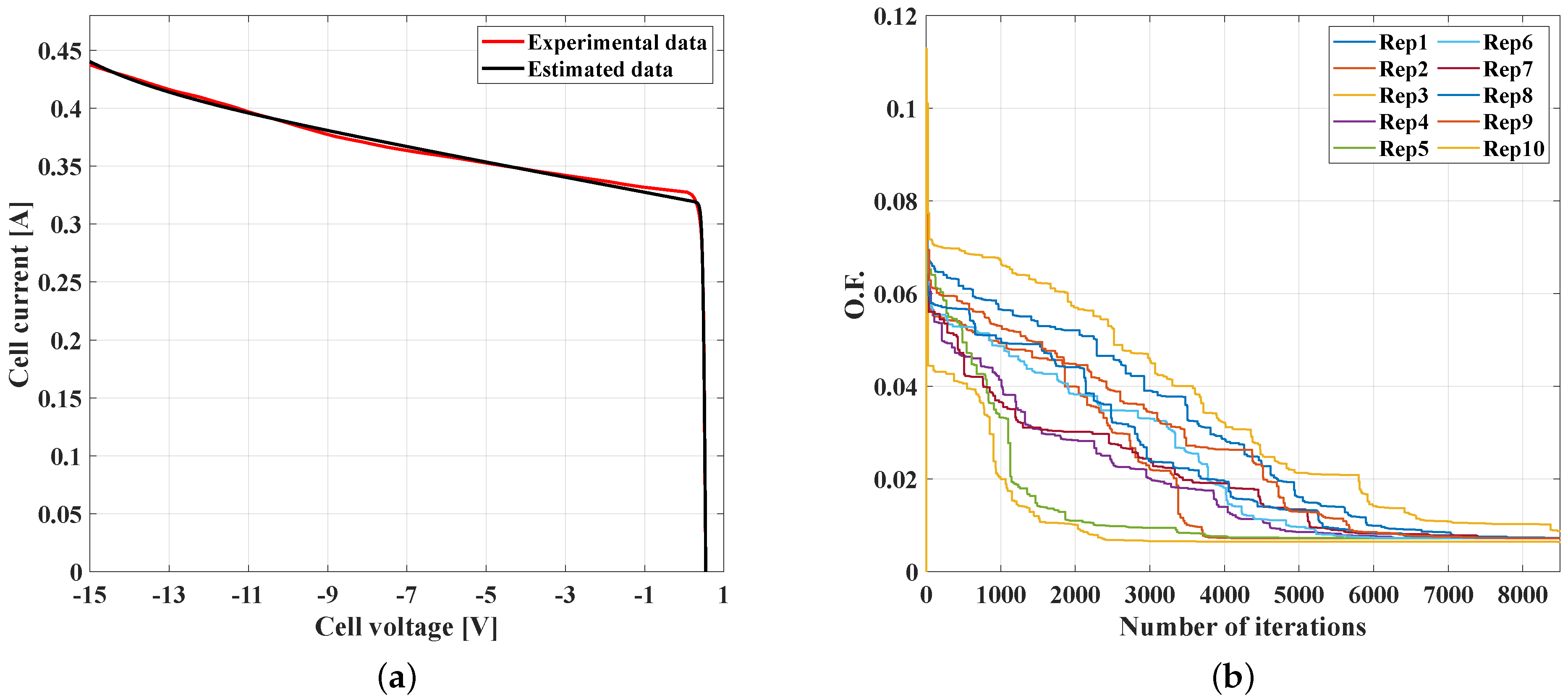
Finally, Figure 13a and Figure 14a compare the estimated I–V curves of Cell 1 and Cell 2 with the experimental data, respectively. Those comparison put into evidence the satisfactory performance of the Bishop model, at the second quadrant, with the parameters estimated using the proposed GA. Thus, this approach provides a much more accurate solution than that obtained using the Bishop parameters reported in [18] for those real PV cells. Moreover, Figure 13b and Figure 14b report a representative sample of the convergence path for the estimation of Cells 1 and 2 parameters, respectively. In both figures, we can observe the consistent decrement of the O.F. as the number of iterations increases, which, after 7000 iterations, forces all solution paths to reach a similar value to the O.F., thus providing a similar accuracy in the second-quadrant reproduction.
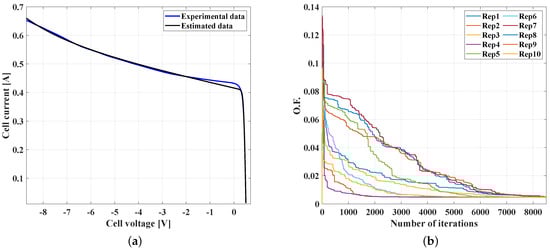
Figure 13.
Parameter estimation results for Cell 1 (mc-SI) using the Bishop model: (a) comparison of I–V curves using the best solution and (b) convergence results for a sample of 10 repetitions.
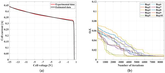
Figure 14.
Parameter estimation results for Cell 2 (pc-SI) using the Bishop model: (a) comparison of I–V curves using the best solution and (b) convergence results for a sample of 10 repetitions.
4.3. Summary of the Proposed Procedure
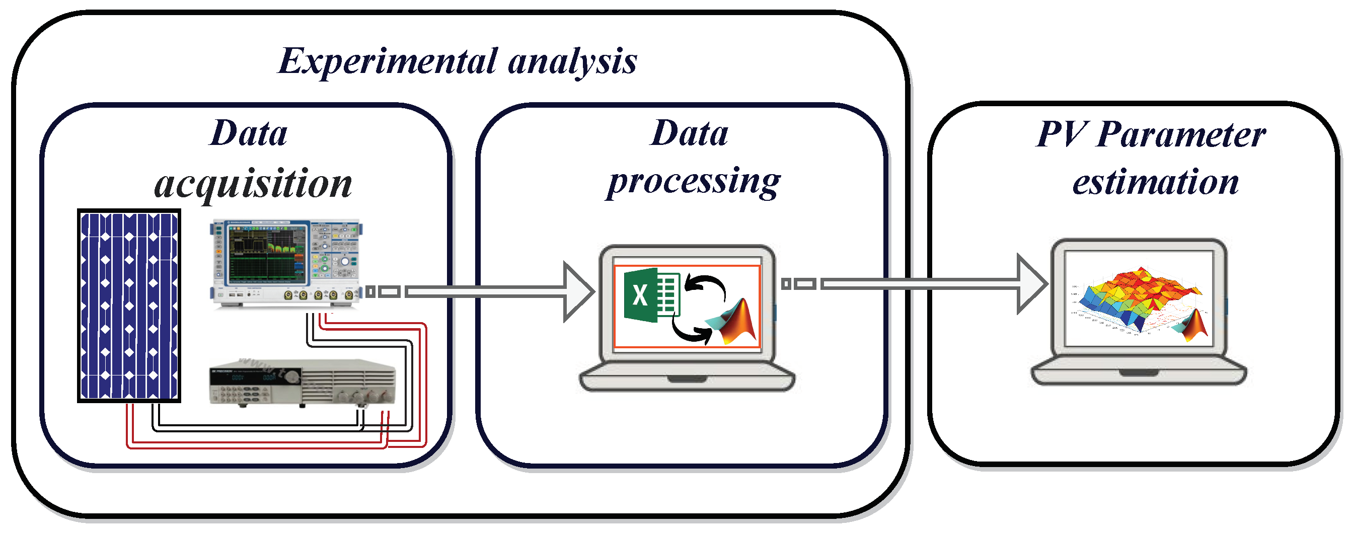
Figure 15 outlines the proposed methodology for estimating the parameters of a photovoltaic cell, considering the behavior in the first and second quadrant, which has two stages: experimental stage and parameter estimation of the model. The following subsections briefly summarize each stage.
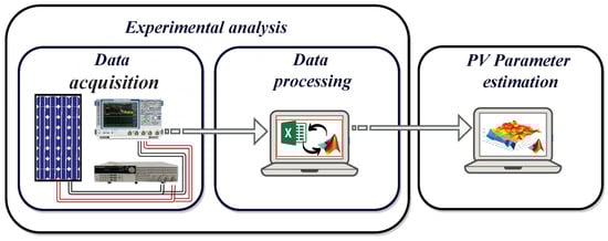
Figure 15.
Summary of the proposed methodology.
4.3.1. Experimental Analysis
This was performed by analyzing the panel I–V data without shading, then exposing a single cell of the panel to partial shading; for this work, we defined a 50% of the cell area. Subsequently, the I–V data must be mathematically manipulated to obtain the I–V curve for the shaded cell. This stage is explained in detail in Section 4.1.
4.3.2. PV Parameter Estimation
The estimation of Bishop’s model parameters requires, in addition to the curves of the experimental stage, the definition of the search ranges for each parameter, which depends on the cell’s technology. In this work, a range is proposed for the technologies used in the tests in Table 2 and Table 8 (mc-SI and pc-SI); however, the search ranges must be investigated for different technologies.
Then, an optimization technique was used to solve the PV parameter estimation problem. This work focused on the GA presented in Section 3.1, which required to define the algorithm parameters, such as number of maximum iterations , number of maximum non-improvement and population size p. This process was performed by using a PSO algorithm to find , and p, thus ensuring a correct behavior of the genetic algorithm; the estimation process is summarized in the flowchart of Figure 5. This estimation process was coded in MATLAB, without using any genetic or optimization toolboxes, which enabled us to optimize the performance of both GA and PSO. Finally, the function that relates the cell voltage and current is an implicit expression; thus, it was solved using the Newton–Raphson method.
The validation of the estimation process was performed by running several repetitions of the parameters estimation. Then, that information was used to calculate accuracy metrics associated to each parameter, the evaluation of the objective function, the execution time and some error measurements, such as those presented in Table 9, Table 10 and Table 11. In this work, RMSE, MAPE and MBE were used to confirm the estimation accuracy.
5. Discussion and Conclusions
Comparing the results of the two stages of the parameter estimation, it was established that the estimation of the complete set of parameters of the Bishop model achieved a better performance than that obtained by estimating only the five SDM parameters and using the second-quadrant parameters reported in [18].
A comparison of the parameter estimation results (Stages 1 and 2) shows that the parameters for the first quadrant were similar for both Cell 1 and Cell 2. The most significant difference in the estimation stages was , which affected the second quadrant behavior in the Bishop model. For that parameter, Cell 1 exhibited differences of between SDM and the Bishop model from its mean values (see Table 3 and Table 10) and from the best results (see Table 5 and Table 9). For Cell 2, those values were and , respectively. This analysis shows that I–V experimental curves, which include the first and second quadrant, are necessary for estimating the parameters of the Bishop model.
This study found differences in the behavior of the I–V curve of mc-SI and pc-SI cells at important points, such as the short-circuit current and the maximum power point . Those variations are reflected in the estimation of the parameters of the Bishop model, as shown in Table 9. Such differences are noticeable not only in the first quadrant, but also in the second quadrant, since the three parameters defining that behavior (a, m and ) show considerable variations depending on the type of cell technology. Therefore, not only parameters but also search ranges should be defined according to the technology of the cells under analysis.
It is important to emphasize that the parameters of the first quadrant also affected both the result of estimating the parameters of the second quadrant and the reproduction of I–V curve in that quadrant; therefore, using values taken from the literature can introduce significant errors in the estimation of the I–V curve. Thus, the solution presented in this paper is a tool to improve the analysis of the cell when it is exposed to partial shading, enabling an accurate representation using the Bishop model. In this way, tools oriented to quantifying shading losses and studies of degradation caused by hot-spots and aging, among other issues, can be developed by using the proposed methodology; this providing a suitable compromise between accuracy and complexity.
Finally, future studies should be focused on evaluating the performance of other optimization techniques for estimating the parameters of photovoltaic cells, for both the first and second quadrant, using the Bishop model. Moreover, performing experiments on a large number of commercial PV cells with different technologies (thin-film, bi-facial and PERC, among others) could be useful for the scientific community, since accurate parameters for both the first and second quadrant could be provided. On the other hand, it is important to evaluate the performance of the proposed approach by considering dynamic operating conditions in terms of temperature and irradiance.
Author Contributions
Conceptualization, B.J.R.-C., J.M., C.A.R.-P., L.A.T.-G. and M.L.O.-G.; methodology, B.J.R.-C., J.M., C.A.R.-P., L.A.T.-G. and M.L.O.-G.; software, B.J.R.-C. and J.M.; validation, B.J.R.-C., J.M., C.A.R.-P., L.A.T.-G. and M.L.O.-G.; writing—original draft preparation, B.J.R.-C. and J.M.; writing—review and editing, B.J.R.-C., J.M., C.A.R.-P., L.A.T.-G. and M.L.O.-G. All authors have read and agreed to the published version of the manuscript.
Funding
This research study and the APC were funded by Minciencias—Ministerio de Ciencia, Tecnología e Innovación—Instituto tecnológico Metropolitano, Universidad Nacional de Colombia and Universidad del Valle, under the research project Estrategias de dimensionamiento, planeación y gestión inteligente de energía a partir de la integración y la optimización de las fuentes no convencionales, los sistemas de almacenamiento y cargas eléctricas, que permitan la generación de soluciones energéticas confiables para los territorios urbanos y rurales en Colombia” (Minciencias code 71148), which belongs to the research program “Estrategias para el desarrollo de sistemas energéticos sostenibles, confiables, eficientes y accesibles para el futuro de Colombia” (Minciencias code 1150-852-70378, Hermes code 46771).
Institutional Review Board Statement
Not applicable.
Informed Consent Statement
Not applicable.
Data Availability Statement
The data used in this study are reported in the paper figures and tables.
Acknowledgments
The authors thank the Facultad de Ingenierías of the Instituto Tecnológico Metropolitano (ITM), the Facultad de Minas (Sede Medellín) of the Universidad Nacional de Colombia, and the Escuela de Ingeniería Eléctrica y Electrónica of the Universidad del Valle.
Conflicts of Interest
The authors declare no conflict of interest.
Abbreviations
The following abbreviations are used in this manuscript:
| PV | photovoltaic |
| mc-SI | monocrystalline silicon |
| pc-SI | polycrystalline silicon |
| SDM | single-diode model |
| DDM | double-diode model |
| PVSIM | software program utilized by SunPower to predict the amount of energy a solar power system |
| GA | genetic algorithm |
| PSO | particle swarm optimization |
| RMSE | root mean square error |
| MAPE | mean absolute percentage error |
| MBE | mean bias error |
| current of the cell | |
| photoinduced current | |
| saturation current of the diode | |
| shunt resistance current | |
| voltage across the diode | |
| shunt resistance | |
| series resistance | |
| ideality factor | |
| k | Boltzman constant |
| q | electron charge |
| T | cell temperature |
| breakdown voltage | |
| m | avalanche exponent |
| a | fraction of the ohmic current related to the breakdown of the semiconductor |
References
- Al-Shetwi, A.Q.; Sujod, M.Z.; Blaabjerg, F. Low voltage ride-through capability control for single-stage inverter-based grid-connected photovoltaic power plant. Sol. Energy 2018, 159, 665–681. [Google Scholar] [CrossRef] [Green Version]
- Polman, A.; Knight, M.; Garnett, E.C.; Ehrler, B.; Sinke, W.C. Photovoltaic materials: Present efficiencies and future challenges. Science 2016, 352, aad4424. [Google Scholar] [CrossRef] [Green Version]
- Georgijevic, N.L.; Jankovic, M.V.; Srdic, S.; Radakovic, Z. The detection of series arc fault in photovoltaic systems based on the arc current entropy. IEEE Trans. Power Electron. 2016, 31, 5917–5930. [Google Scholar] [CrossRef]
- Babu, B.C.; Gurjar, S. A novel simplified two-diode model of photovoltaic (PV) module. IEEE J. Photovoltaics 2014, 4, 1156–1161. [Google Scholar] [CrossRef]
- Tamrakar, V.; Gupta, S.; Sawle, Y. Single-diode and two-diode PV cell modeling using Matlab for studying characteristics of solar cell under varying conditions. Electr. Comput. Eng. Int. J. (ECIJ) 2015, 4, 67–77. [Google Scholar] [CrossRef]
- Ishaque, K.; Salam, Z. A comprehensive MATLAB Simulink PV system simulator with partial shading capability based on two-diode model. Sol. Energy 2011, 85, 2217–2227. [Google Scholar] [CrossRef]
- Barroso, J.S.; Correia, J.; Barth, N.; Ahzi, S.; Khaleel, M. A PSO algorithm for the calculation of the series and shunt resistances of the PV panel one-diode model. In Proceedings of the 2014 International Renewable and Sustainable Energy Conference (IRSEC), Ouarzazate, Morocco, 17–19 October 2014; pp. 1–6. [Google Scholar]
- Bastidas-Rodriguez, J.D.; Petrone, G.; Ramos-Paja, C.A.; Spagnuolo, G. A genetic algorithm for identifying the single diode model parameters of a photovoltaic panel. Math. Comput. Simul. 2017, 131, 38–54. [Google Scholar] [CrossRef]
- Ma, J.; Ting, T.; Man, K.L.; Zhang, N.; Guan, S.U.; Wong, P.W. Parameter estimation of photovoltaic models via cuckoo search. J. Appl. Math. 2013, 2013, 362619. [Google Scholar] [CrossRef]
- Bai, J.; Cao, Y.; Hao, Y.; Zhang, Z.; Liu, S.; Cao, F. Characteristic output of PV systems under partial shading or mismatch conditions. Sol. Energy 2015, 112, 41–54. [Google Scholar] [CrossRef]
- Hosseini, S.; Taheri, S.; Farzaneh, M.; Taheri, H. An approach to precise modeling of photovoltaic modules under changing environmental conditions. In Proceedings of the 2016 IEEE Electrical Power and Energy Conference (EPEC), Ottawa, ON, Canada, 12–14 October 2016; pp. 1–6. [Google Scholar]
- Elbaset, A.A.; Ali, H.; Abd El Sattar, M. New seven parameters model for amorphous silicon and thin film PV modules based on solar irradiance. Sol. Energy 2016, 138, 26–35. [Google Scholar] [CrossRef]
- Bana, S.; Saini, R. A mathematical modeling framework to evaluate the performance of single diode and double diode based SPV systems. Energy Rep. 2016, 2, 171–187. [Google Scholar] [CrossRef] [Green Version]
- Silvestre, S.; Boronat, A.; Chouder, A. Study of bypass diodes configuration on PV modules. Appl. Energy 2009, 86, 1632–1640. [Google Scholar] [CrossRef]
- Yaqoob, S.J.; Saleh, A.L.; Motahhir, S.; Agyekum, E.B.; Nayyar, A.; Qureshi, B. Author Correction: Comparative study with practical validation of photovoltaic monocrystalline module for single and double diode models. Sci. Rep. 2021, 11, 21822. [Google Scholar] [CrossRef] [PubMed]
- Belhachat, F.; Larbes, C. Modeling, analysis and comparison of solar photovoltaic array configurations under partial shading conditions. Sol. Energy 2015, 120, 399–418. [Google Scholar] [CrossRef]
- Díaz-Dorado, E.; Cidras, J.; Carrillo, C. Discrete I–V model for partially shaded PV-arrays. Sol. Energy 2014, 103, 96–107. [Google Scholar] [CrossRef]
- Bishop, J. Computer simulation of the effects of electrical mismatches in photovoltaic cell interconnection circuits. Sol. Cells 1988, 25, 73–89. [Google Scholar] [CrossRef]
- Kawamura, H.; Naka, K.; Yonekura, N.; Yamanaka, S.; Kawamura, H.; Ohno, H.; Naito, K. Simulation of I–V characteristics of a PV module with shaded PV cells. Sol. Energy Mater. Sol. Cells 2003, 75, 613–621. [Google Scholar] [CrossRef]
- King, D.; Dudley, J.; Boyson, W. PVSIM ©: A Simulation Program for Photovoltaic Cells, Modules, and Arrays; Technical Report; Sandia National Labs.: Albuquerque, NM, USA, 1996. [Google Scholar]
- Liu, G.; Nguang, S.K.; Partridge, A. A general modeling method for I–V characteristics of geometrically and electrically configured photovoltaic arrays. Energy Convers. Manag. 2011, 52, 3439–3445. [Google Scholar] [CrossRef]
- Maouhoub, N. Photovoltaic module parameter estimation using an analytical approach and least squares method. J. Comput. Electron. 2018, 17, 784–790. [Google Scholar] [CrossRef]
- Ciulla, G.; Brano, V.L.; Di Dio, V.; Cipriani, G. A comparison of different one-diode models for the representation of I–V characteristic of a PV cell. Renew. Sustain. Energy Rev. 2014, 32, 684–696. [Google Scholar] [CrossRef]
- Nunes, H.; Pombo, J.; Fermeiro, J.; Mariano, S.; do Rosário Calado, M. Particle Swarm Optimization for photovoltaic model identification. In Proceedings of the 2017 International Young Engineers Forum (YEF-ECE), Costa da Caparica, Portugal, 5 May 2017; pp. 53–58. [Google Scholar]
- Montano, J.; Tobón, A.; Villegas, J.; Durango, M. Grasshopper optimization algorithm for parameter estimation of photovoltaic modules based on the single diode model. Int. J. Energy Environ. Eng. 2020, 11, 367–375. [Google Scholar] [CrossRef]
- Benkercha, R.; Moulahoum, S.; Colak, I.; Taghezouit, B. PV module parameters extraction with maximum power point estimation based on flower pollination algorithm. In Proceedings of the 2016 IEEE International Power Electronics and Motion Control Conference (PEMC), Varna, Bulgaria, 25–28 September 2016; pp. 442–449. [Google Scholar]
- Petrone, G.; Ramos-Paja, C.A.; Spagnuolo, G. Photovoltaic Sources Modeling; John Wiley & Sons: Hoboken, NJ, USA, 2017. [Google Scholar]
- El Tayyan, A.A. An approach to extract the parameters of solar cells from their illuminated IV curves using the Lambert W function. Turk. J. Phys. 2015, 39, 1–15. [Google Scholar] [CrossRef]
- Chin, V.J.; Salam, Z.; Ishaque, K. Cell modelling and model parameters estimation techniques for photovoltaic simulator application: A review. Appl. Energy 2015, 154, 500–519. [Google Scholar] [CrossRef]
- Raj, S.; Kumar Sinha, A.; Panchal, A.K. Solar cell parameters estimation from illuminated I-V characteristic using linear slope equations and Newton-Raphson technique. J. Renew. Sustain. Energy 2013, 5, 033105. [Google Scholar] [CrossRef]
- Chatterjee, A.; Keyhani, A.; Kapoor, D. Identification of photovoltaic source models. IEEE Trans. Energy Convers. 2011, 26, 883–889. [Google Scholar] [CrossRef]
- Kler, D.; Goswami, Y.; Rana, K.; Kumar, V. A novel approach to parameter estimation of photovoltaic systems using hybridized optimizer. Energy Convers. Manag. 2019, 187, 486–511. [Google Scholar] [CrossRef]
- Hachana, O.; Hemsas, K.; Tina, G.; Ventura, C. Comparison of different metaheuristic algorithms for parameter identification of photovoltaic cell/module. J. Renew. Sustain. Energy 2013, 5, 053122. [Google Scholar] [CrossRef]
- Ismail, M.S.; Moghavvemi, M.; Mahlia, T. Characterization of PV panel and global optimization of its model parameters using genetic algorithm. Energy Convers. Manag. 2013, 73, 10–25. [Google Scholar] [CrossRef]
- Waly, H.M.; Azazi, H.Z.; Osheba, D.S.; El-Sabbe, A.E. Parameters extraction of photovoltaic sources based on experimental data. IET Renew. Power Gener. 2019, 13, 1466–1473. [Google Scholar] [CrossRef]
- Hamadi, S.A.; Chouder, A.; Rezaoui, M.M.; Motahhir, S.; Kaddouri, A.M. Improved Hybrid Parameters Extraction of a PV Module Using a Moth Flame Algorithm. Sci. Rep. 2021, 10, 2798. [Google Scholar] [CrossRef]
- Tobón, A.; Peláez-Restrepo, J.; Montano, J.; Durango, M.; Herrera, J.; Ibeas, A. MPPT of a photovoltaic panels array with partial shading using the IPSM with implementation both in simulation as in hardware. Energies 2020, 13, 815. [Google Scholar] [CrossRef] [Green Version]
- Mejia, A.F.T. Estimación de los parámetros del modelo de un solo diodo del módulo fotovoltaico aplicando el método de optimización basado en búsqueda de patrones mejorado. Rev. Ing. Univ. Medellín 2021, 20, 13–32. [Google Scholar] [CrossRef]
- Koffi, H.; Kuditcher, A.; Kakane, V.; Armah, E.; Yankson, A.; Amuzu, J. The Shockley five-parameter model of a solar cell: A short note. Afr. J. Sci. Technol. Innov. Dev. 2015, 7, 491–494. [Google Scholar] [CrossRef]
- Rohde-Schwarz. R&S®RTE OSCILLOSCOPE: Specifications. Available online: https://scdn.rohde-schwarz.com/ur/pws/dl_downloads/dl_common_library/dl_brochures_and_datasheets/pdf_1/RTE_dat-sw_en_3607-1494-22_v2500.pdf (accessed on 1 September 2021).
- Zhang, Y.; Lin, P.; Chen, Z.; Cheng, S. A population classification evolution algorithm for the parameter extraction of solar cell models. Int. J. Photoenergy 2016, 2016, 2174573. [Google Scholar] [CrossRef] [Green Version]
- Gong, W.; Cai, Z. Parameter extraction of solar cell models using repaired adaptive differential evolution. Sol. Energy 2013, 94, 209–220. [Google Scholar] [CrossRef]
- Tamrakar, R.; Gupta, A. Extraction of solar cell modelling parameters using differential evolution algorithm. Int. J. Innov. Res. Electr. Electron. Instrum. Control Eng. 2015, 3, 78–82. [Google Scholar] [CrossRef]
- Yoon, Y.; Geem, Z.W. Parameter optimization of single-diode model of photovoltaic cell using memetic algorithm. Int. J. Photoenergy 2015, 2015, 963562. [Google Scholar] [CrossRef] [Green Version]
- Vélez-Sánchez, J.; Bastidas-Rodríguez, J.D.; Ramos-Paja, C.A.; González Montoya, D.; Trejos-Grisales, L.A. A Non-Invasive Procedure for Estimating the Exponential Model Parameters of Bypass Diodes in Photovoltaic Modules. Energies 2019, 12, 303. [Google Scholar] [CrossRef] [Green Version]
- Chen, Z.; Wu, L.; Lin, P.; Wu, Y.; Cheng, S. Parameters identification of photovoltaic models using hybrid adaptive Nelder-Mead simplex algorithm based on eagle strategy. Appl. Energy 2016, 182, 47–57. [Google Scholar] [CrossRef]
- Ishaque, K.; Salam, Z.; Mekhilef, S.; Shamsudin, A. Parameter extraction of solar photovoltaic modules using penalty-based differential evolution. Appl. Energy 2012, 99, 297–308. [Google Scholar] [CrossRef]
- Ma, J. Optimization Approaches for Parameter Estimation and Maximum Power Point Tracking (MPPT) of Photovoltaic Systems. Ph.D. Thesis, University of Liverpool, Liverpool, UK, 2014. [Google Scholar]
- Muhsen, D.H.; Ghazali, A.B.; Khatib, T.; Abed, I.A. A comparative study of evolutionary algorithms and adapting control parameters for estimating the parameters of a single-diode photovoltaic module’s model. Renew. Energy 2016, 96, 377–389. [Google Scholar] [CrossRef]
- Grisales-Noreña, L.F.; Gonzalez Montoya, D.; Ramos-Paja, C.A. Optimal sizing and location of distributed generators based on PBIL and PSO techniques. Energies 2018, 11, 1018. [Google Scholar] [CrossRef] [Green Version]
- Montano, J.; Mejia, A.F.T.; Rosales Muñoz, A.A.; Andrade, F.; Garzon Rivera, O.D.; Palomeque, J.M. Salp Swarm Optimization Algorithm for Estimating the Parameters of Photovoltaic Panels Based on the Three-Diode Model. Electronics 2021, 10, 3123. [Google Scholar] [CrossRef]
- Silvestre, S.; Chouder, A. Effects of shadowing on photovoltaic module performance. Prog. Photovoltaics Res. Appl. 2008, 16, 141–149. [Google Scholar] [CrossRef]
- Batzelis, E.I.; Routsolias, I.A.; Papathanassiou, S.A. An explicit PV string model based on the lambert W function and simplified MPP expressions for operation under partial shading. IEEE Trans. Sustain. Energy 2013, 5, 301–312. [Google Scholar] [CrossRef]
- Fezzani, A.; Mahammed, I.H.; Said, S. MATLAB-based modeling of shading effects in photovoltaic arrays. In Proceedings of the 2014 15th International Conference on Sciences and Techniques of Automatic Control and Computer Engineering (STA), Hammamet, Tunisia, 21–23 December 2014; pp. 781–787. [Google Scholar]
- Orozco-Gutierrez, M.; Ramirez-Scarpetta, J.; Spagnuolo, G.; Ramos-Paja, C. A method for simulating large PV arrays that include reverse biased cells. Appl. Energy 2014, 123, 157–167. [Google Scholar] [CrossRef]
- Belhadj, C.A.; Banat, I.; Deriche, M. A detailed analysis of photovoltaic panel hot spot phenomena based on the bishop model. In Proceedings of the 2017 14th International Multi-Conference on Systems, Signals & Devices (SSD), Marrakech, Morocco, 28–31 March 2017; pp. 222–227. [Google Scholar]
- Mahammed, I.H.; Arab, A.H.; Bakelli, Y.; Khennene, M.; Oudjana, S.H.; Fezzani, A.; Zaghba, L. Outdoor study of partial shading effects on different PV modules technologies. Energy Procedia 2017, 141, 81–85. [Google Scholar] [CrossRef]
- Guerriero, P.; Codecasa, L.; d’Alessandro, V.; Daliento, S. Dynamic electro-thermal modeling of solar cells and modules. Sol. Energy 2019, 179, 326–334. [Google Scholar] [CrossRef]

Publisher’s Note: MDPI stays neutral with regard to jurisdictional claims in published maps and institutional affiliations. |
© 2022 by the authors. Licensee MDPI, Basel, Switzerland. This article is an open access article distributed under the terms and conditions of the Creative Commons Attribution (CC BY) license (https://creativecommons.org/licenses/by/4.0/).