A New Technique of Eliminating the Actual Plasma Background When Calibrating Emission Spectrometers with a CCD Recording System

Abstract

This research focuses on the development of a new technique of emission spectral analysis designed to accurately account for the background radiation. The technique enables the evaluation of background radiation while being unaffected by its spectral shape. This is possible through the use of standard data obtained in an analytical-line-recording process performed by light-intensity-to-electric-signal converters such as CCDs, PMTs, photodiodes, etc. This technique, when applied at a set RMS deviation of the analytical-line-radiation intensity, reduces the random error of a determined low impure-element concentration due to the optimal calibration-line slope. In areas of high concentrations, an accurate accounting of the background does little to affect the emission spectrometer’s measurement accuracy. This technique also allows the replication of calibration curves in spectrometers of the same type by a linear-intensity conversion with only two standard samples required. The technique was tested on SPAS-02 and SPAS-05 commercial spark spectrometers. The testing fully confirmed the aforementioned advantages of the developed technique. The authors also determined the applicability conditions of the conventional emission-spectrometer-recalibration method by a linear conversion of the analytical-line intensity.

1. Introduction

Emission spectral analysis is the most widespread express method to estimate elemental composition [1,2,3,4,5] in various industries [6,7,8]. Most of the modern emission spectrometers utilize the so-called charge-coupled devices (CCDs) as an optical radiation-recording system [9,10,11,12,13,14,15], and different types of gas-discharge plasma are used for optical excitation [5,16].

Setting up emission spectrometers includes, above all, calibration graphs that plot the dependence of an element’s analytical-line intensity on its concentration in an analyzed sample, or an inverse function that plots the concentration dependence on intensity. To determine the impure-element content in a sample, it is necessary to measure the analytical-line intensity of this element. For applications using a CCD recording system, this means summing the digitized charge values of individual CCD pixels, on which the image of the analytical line of a selected impure element falls. At this point it is necessary, if possible, to eliminate the signal, which corresponds to the intensity of the plasma background radiation independent of the concentration of a given impure element (it may be plasma electron bremsstrahlung, molecular bands of plasma-forming gases, etc.).

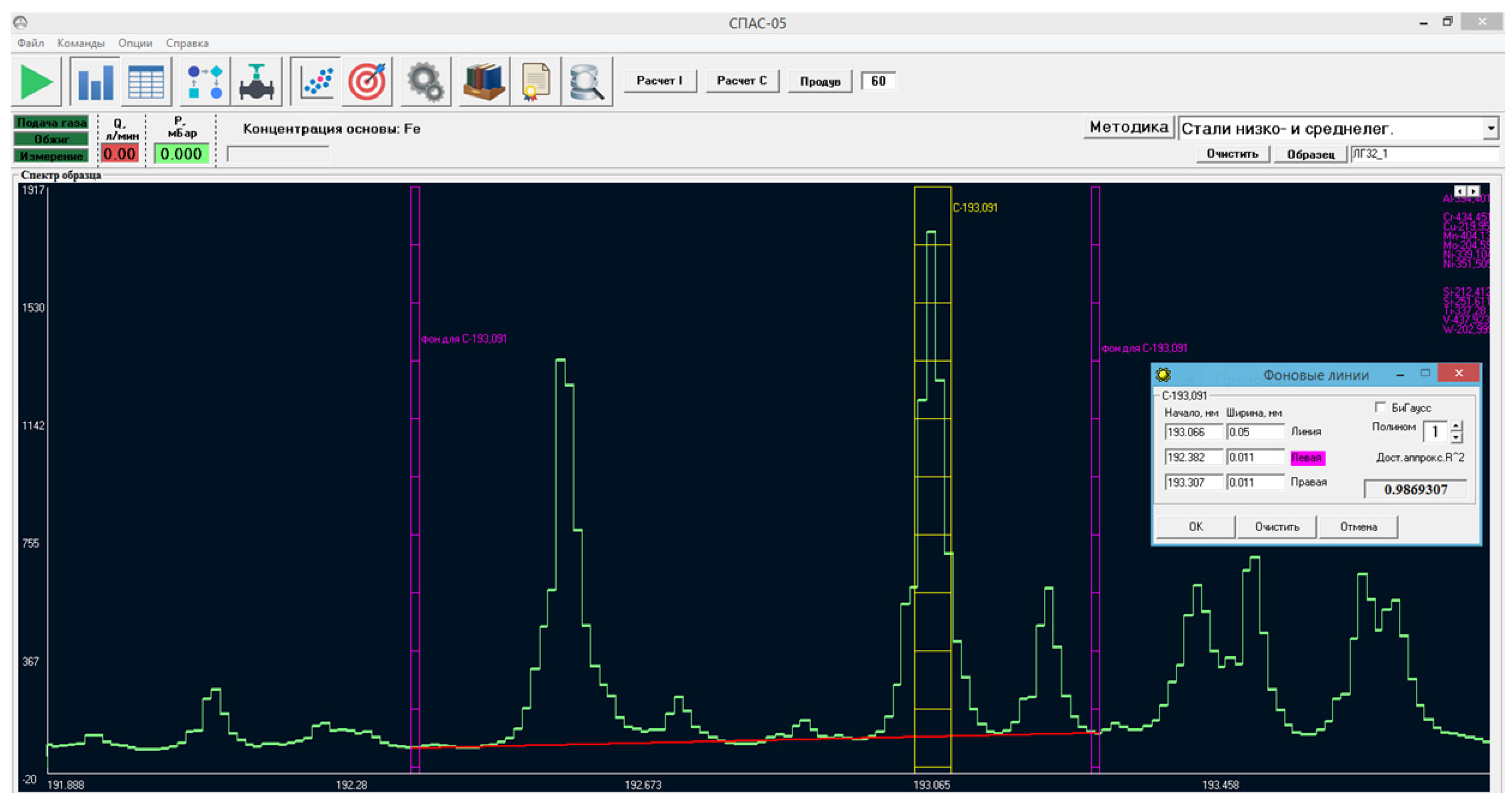
In modern spectrometers, this is performed, as a rule, according to the following algorithm [17,18]. In the corresponding spectrometer’s software window, the pixels on which the image of the analytical line falls are specially marked (see Figure 1). As an example, Figure 1 shows the software window of the SPAS-05 emission spectrometer produced by Active Co. Ltd., Saint Petersburg, Russia, in the CI 193.09 nm analytical carbon-line area (see Appendix A for brief technical spectrometer specifications). The CCD pixels on which the image of this line falls are within the yellow rectangle. In this case, to subtract plasma background radiation to the left and right of the analytical line (sometimes only on one side), an area in the spectrum that is free from the spectral lines of all elements is selected. Then, the set of intersection points of the right and left reference frames (see purple lines Figure 1) and the plasma spectrum envelope are connected by a polynomial of a degree (see the red line Figure 1), which we will refer to as the cutoff line. The analytical signal below this line is considered the plasma background and is neglected when calculating.

Under this approach, the unknown spectral shape of plasma radiation at the analytical-line location cannot ultimately coincide with the envelope shape and, thus, the plasma background is inaccurately accounted for. This leads to the fact that at zero concentration of the given impurity, the intensity of its analytical line as measured by the spectrometer is non-zero. This, in turn, causes significant and uncontrollable device-to-device distortions of the calibration curves in the area of low impurity concentrations, which further results in a slope decline in the calibration curve for the case of the intensity dependence on concentration, (or an increase for the case of the inverse function), and a forced increase in the degree of the polynomial that is approximating the calibration curve.

These effects lead to a lower detection limit and an increase in the RMS deviation of the concentration measurements. They are, inter alia, one of the factors that impede the replication of the calibration curves of one device in other devices of the same type.

This paper is dedicated to the development of this algorithm in order to accurately evaluate the actual background at the element’s analytical-line location using standard data captured by the CCD recording system, thus eliminating the above-listed deficiencies.

The so-called spectrometer-recalibration algorithm was separately studied when implementing the developed method of accurate accounting for the background signal (calibration adjustments due to changes in the in-service-spectrometer characteristics). Under the most general assumptions about the principles of signal formation of the spectrometer recording system, we found conditions under which there is a linear relationship between the recorded analytical-line intensities before and after the changes in the spectrometer parameters.

2. Materials and Methods

Key formulas.Accurate accounting for the background signal. We assume that to determine the analytical-line intensity it is necessary to sum the signals $M$ of the CCD pixels. In the given case study, these are pixels located within the yellow sector in Figure 1. The $N$ number of standard samples (SS) is used to construct the calibration for this element. We number them in ascending order of concentration, i.e., the lower standard is №1, etc. Thus, the analytical-line intensity of a certain wavelength $I$ of some element, when the standard sample $i$ is used, transformed into the signal of the recording system is:

$$I_i={\sum }_{k=1}^M{I}_{ki},$$

(1)

where $I_{ki}$ is the intensity in the pixel $k$ of the analytical line of the element being determined in the analysis of the standard sample $i$. We should note that the intensities are calculated considering the model background (the part of the intensity that is lower than the cutoff line is omitted in each pixel in Figure 1). The relative (or the absolute, according to the analytical task) impurity concentration in sample $i$ is $C_i$. The standard procedure for plotting the calibration is to use the data sets $I_i,C_i$, $i=1,\dots ,N$ to plot the dependence

$$C=F(I),$$

(2)

where $F(I)$ is usually a polynomial of no greater than degree 4. It should be noted that we previously discussed the dependence of the analytical-line intensity on the element concentration, which is justified from a physical point of view, although Equation (2) is an inverse function. The point is that, from a mathematical point of view, it is Equation (2) for which the process of determining the unknown concentration by the measured intensity is trivial, while for the inverse dependence $I=F^{-1}(C)$, it is necessary to solve an algebraic equation.

As indicated, the non-coincidence of the shape of the actual plasma background radiation (which is unknown in advance) with the cutoff-line shape results in distortions of the calibration curve at low concentrations $C$; as such, the calibration dependence does not meet the requirement of zero intensity at zero concentration of the determined element.

Therefore, we will proceed as follows. The intensity $I_{ki}$ consists of the actual analytical signal $I_{ak}$, determined by the impurity in the sample, and $I_{fk}$, which is the difference in the pixel $k$ between the intensity of the actual plasma background and the background that has the shape of the cutoff line (hereinafter we will refer to this difference as simply the background). The latter weakly depends on a standard sample number, i.e., on the content of the impurities determined within it. This dependence will be neglected. Thus, for the standard sample number $i$, we have:

$$I_{ki}=I_{aki}+I_{fk}.$$

(3)

Summing Equation (3) by pixels, we have:

$$I_i=I_{ai}+I_F,$$

(4)

where $I_{ai}=\sum _{k=1}^M{I}_{aki}$; $I_F=\sum _{k=1}^M{I}_{fk}$ is the actual (not the measured) intensity of the analytical line of standard sample $i$ and the background at this line location, therefore, is converted by the recording system into an electrical signal. To calculate value $I_F$ we will compile dataset $\Delta I_i=I_i-I_1=I_{ai}-I_{a1}$; $\Delta C_i=C_i-C_1$; $i=1,\dots ,N$. We should note that the dataset also has $N$ values of $\Delta I_i$ and $\Delta C_i$, and there is no value $I_F$. Using an ordinary least-squares technique, we approximate this dataset by a polynomial

$$\Delta C=F_a(\Delta I).$$

(5)

By determining the values in Equation (5), it must be true that if $C=0$, i.e., when $\Delta C=-C_1$and $I_a=0$, then the equality is true:

$$\Delta I=\Delta I_0\equiv I_F-I_1.$$

(6)

Thus, we calculate value $I_F$ from the correlation:

$$I_F=\Delta I_0+I_1,$$

(7)

where $\Delta I_0$is the equation root:

$$F_a(\Delta I_0)=-C_1.$$

(8)

After we made the appropriate adjustment to the plasma background value $I_F$, the calibration is being plotted at the analytical-line location.

$$C=F_A(I-I_F)$$

(9)

In this case, if $C=0$, then $I=I_F$, because, by the definition of the functions $F_A$ and $F_a$, the following is true:

$$F_A(I-I_F)=F_a(I-I_1)+C_1,$$

(10)

and $F_A(0)=F_a(I_F-I_1)+C_1=0$.

It is necessary to note the following. When plotting the curve $F_a(I-I_1)$, we should apparently use the functional:

$$S_c=\sum _{i=1}^N\frac{{[C_i-C_1-F_a(I_i-I_1)]}^2}{C_i{}^2},$$

(11)

rather than

$$S=\sum _{i=1}^N{[C_i-C_1-F_a(I_i-I_1)]}^2,$$

(12)

since, in the functional $S$, the contribution of the lowest concentration points (when the standard sample index $i$ is low due to the numbering method) is significantly less than the contribution of the points with a high index $i$ (high-concentration points) due to a greater impurity concentration, and its use may result in significant inaccuracies when determining a relatively small value $I_F<I_1$.

3. Results

Key formulas. Calibration-curve recalibration accounting for background precise value. As it is known, due to diverse physical reasons, the continuous operation of an emission spectrometer may cause a change in the spectral-transmission coefficient of the device. This may be, for instance, due to contamination of the slit-light system’s optical elements, or the size reduction of the entrance slit itself (also due to contamination).

Besides, changes may occur in the parameters of the spectrometer systems that are responsible for impure-atom emission from the analyzed sample and their optical excitation. The influencing factors may include the changes over time in the parameters of the electronic units of the spectrum-excitation system when using spark and arc spectrometers, changes in the shape of the electrodes due to various technological reasons, etc.

Finally, the changes may affect sensitive element parameters of the recording system and the system of its signal conversion, for example, as a result of wavelength-selective aging of the radiation receivers of a spectrometer recording system, i.e., a CCD sensitivity shift, etc.

This necessitates the adjustment of calibration curves, which is called recalibration. This procedure is of great importance to ensure the emission spectrometers operate correctly. The existing methods of emission-spectrometer recalibration are based on the following assumptions:

• The calibration-curve shape of the dependence of the measured (not emitted by impure atoms in the light source) analytical-line intensity of the impure atoms on their concentration in an analyzed sample under the parameter changes of an in-service spectrometer is constant [17,18,19,20,21];
• The relationship between the measured analytical-line intensities before and after the spectrometer’s parameter changes is linear [17,18,19,20,21].

As experience with various brands of spectrometers shows, the first assumption is quite valid (we will discuss it in detail further on). At the same time, the second assumption is apparently not always valid. As a rule, the authors who assume a linear dependence between the analytical-line intensities before and after the spectrometer parameters change do not analyze the reasons for this relationship and the area of its application. We will conduct such an analysis below. Firstly, we will determine how these linear-conversion parameters are related to the spectrometer parameters. Secondly, we will determine the conditions under which the relationship between the intensities $I$ and $I^{\prime }$ is linear.

We consider the recalibration algorithm in the case when the measured intensity $I$ of the analytical line of a particular wavelength and the impurity concentration in SS $C$ are related by Equation (2). After the spectral-transmission coefficient has been changed, this analytical-line intensity $I^{\prime }$ (similarly, all other values related to the spectrometer with a modified transmission coefficient will also be indicated with a stroke) of some impure element at the same impurity concentration is changed. It is related to intensity $I$ by the correlation:

$$I=F_I(I^{\prime }),$$

(13)

where $F_I(I^{\prime })$ is some yet unknown function.

Then, for the spectrometer with a modified transmission coefficient, there are correlations to Equations (5) and (9):

$$\Delta C={F^{\prime }}_a(I^{\prime }-{I^{\prime }}_1);C={F^{\prime }}_A(I^{\prime }-{I^{\prime }}_F).$$

(14)

We suppose that assumption (1) is satisfied, i.e., the shape of calibration curves is the same, and the equality is valid:

$${F^{\prime }}_a(I^{\prime })=F_a[F_I(I^{\prime })],$$

where $z$ is the arbitrary analytical-line intensity.

As shown in the Appendix A, this requires that analytical-line-intensity-formation conditions stay unchanged before the spectrometer slit-light entrance system. In this case, the correlation between the intensity from the optical-system radiation entrance to the device’s recording system, as well as the parameters of radiation conversion into an electric signal by this recording system may vary. Otherwise, the shape of the calibration curves may differ significantly and recalibration using this algorithm will be impossible.

Then, knowing that for an arbitrary sample (standard or unknown-composition sample) due to the function definition of $F_A(x)$, the following is fulfilled:

$$F_A(I-I_F)=F_A[F_I(I^{\prime })-F_I({I^{\prime }}_F)]$$

We get:

$$I-I_F=F_I(I^{\prime })-F_I({I^{\prime }}_F).$$

(15)

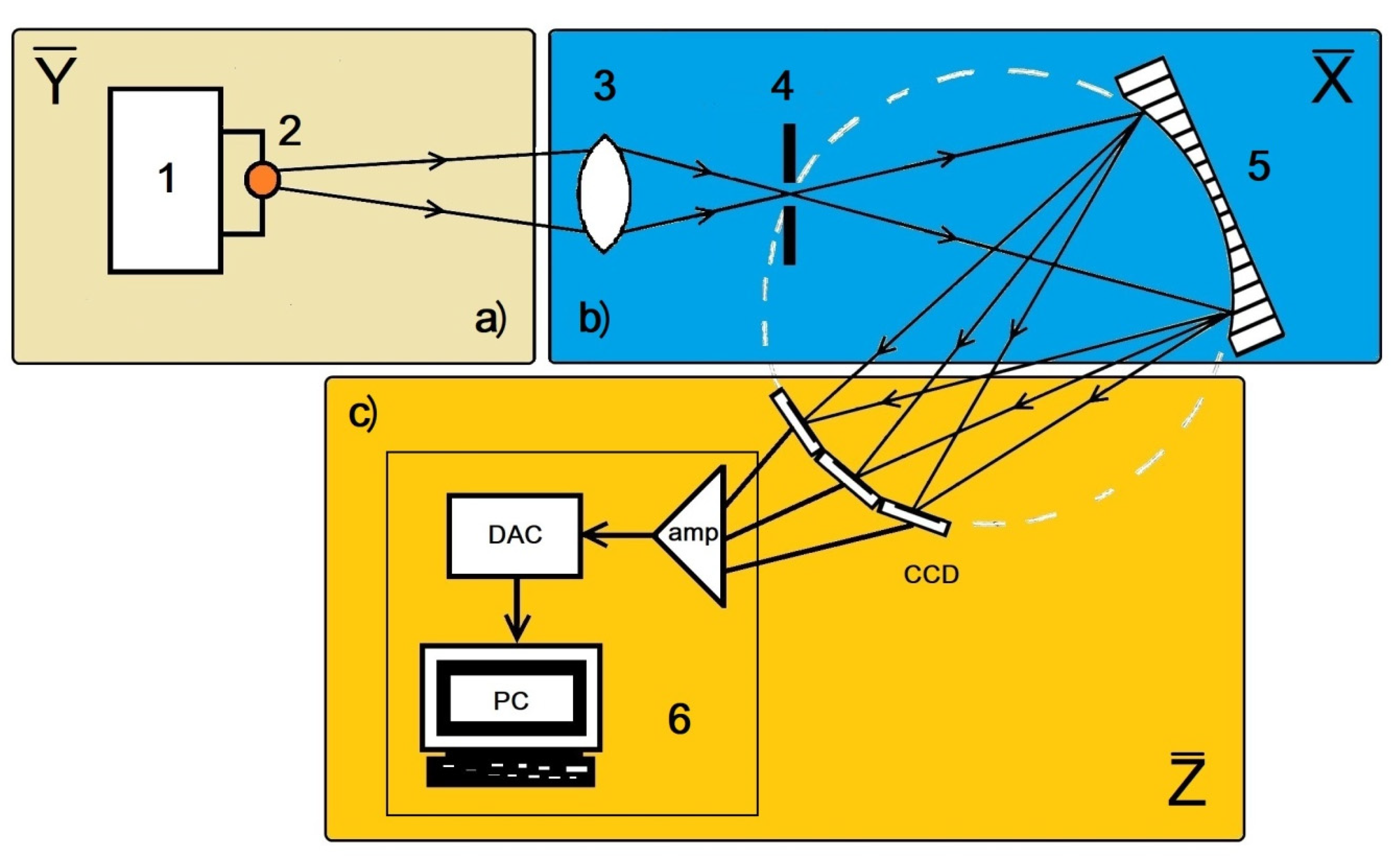
We divide all the independent parameters that determine the measured analytical-line intensity into three groups (see Figure 2):

• The parameters that determine the spectral-transmission coefficient of the spectrometer (let their number be $s$).
• The parameters that determine the analytical-line intensity before it enters the slit-light entrance system (their number is $g$).
• The parameters that determine the conversion coefficient of incoming CCD radiation intensity as a digitized signal that is processed by the spectrometer software (their number is $m$).

We shall indicate them as (a) $(x_1,\dots ,x_s)=\overrightarrow{X}$, (b) $(y_1,\dots ,y_g)=\overrightarrow{Y}$ and (c) $(z_1,\dots .,z_m)=\overrightarrow{Z}$. We also assume that the analytical-line intensity is $I_0(\overrightarrow{Y})$ before it enters the spectrometer’s slit-light entrance system, and that it is $I_l(\overrightarrow{X},\overrightarrow{Y})$ in the CCD plane before conversion by the recording system. Thus, $I$ is the intensity $I_l$ converted by the recording system with the conversion coefficient $K_C(\overrightarrow{X},\overrightarrow{Y},\overrightarrow{Z})$, which generally also dependents on the incoming CCD radiation intensity. The radiation in turn depends on the parameters $\overrightarrow{X}, \overrightarrow{Y}$. Thus, the relation between the values $I_0,I_l,I$ is as follows:

$$\frac{I_l}{I_0}=K[\overrightarrow{X},I_0(\overrightarrow{Y})];I=K_C(\overrightarrow{Z},I_l)I_l=K_C(\overrightarrow{X},\overrightarrow{Y},\overrightarrow{Z})I_l$$

(16)

where $K[\overrightarrow{X},I_0(\overrightarrow{Y})]$ is the spectrometer-transmission coefficient. Now we consider the most general case and assume that the transmission coefficient depends not only on the parameter $\overrightarrow{X}$, but also on the intensity $I_0$, whereas the conversion coefficient depends on $I_l(\overrightarrow{X},\overrightarrow{Y})$.

Now we identify Equation (13) based on the most general correlations. As a rule, while using modern emission spectrometers, a dark signal of the recording system is automatically accounted for. Nevertheless, we assume that due to, for instance, a change in the dark signal (and noise) of the CCD recording-system receivers during continuous operation of the spectrometer, there is some additional signal $I_n(\overrightarrow{X})$, that contributes to the measured intensity. Under these assumptions, the correlation between the analytical-line intensity, before it enters the spectrometer slit-light entrance system, and the recording-system signal at the wavelength of this analytical line in the agreed notations is as follows:

$$I=K_C(\overrightarrow{X},\overrightarrow{Y},\overrightarrow{Z})\left\{K[\overrightarrow{X},I_0(\overrightarrow{Y})]·I_0(\overrightarrow{Y})+I_n(\overrightarrow{X})\right\}.$$

(17)

After parameters $\overrightarrow{X},\overrightarrow{Y},\overrightarrow{Z}$ are changed (into parameters $\overrightarrow{X^{\prime }},\overrightarrow{Y^{\prime }},\overrightarrow{Z^{\prime }}$) all the intensities in this correlation will be changed, and we obtain:

$$I^{\prime }=K_C(\overrightarrow{X},\overrightarrow{Y},\overrightarrow{Z})\{K[\overrightarrow{X^{\prime }},I_0(\overrightarrow{Y^{\prime }})]·I_0(\overrightarrow{Y^{\prime }})+I_n(\overrightarrow{X^{\prime }})\},$$

(18)

where strokes denote the values after the change in parameters. As seen from Equation (17), function $I(\overrightarrow{X},\overrightarrow{Y},\overrightarrow{Z})$ depends on $s+g+m$ of independent scalar arguments. First, we assume that the spectrometer-transmission coefficient does not depend on the intensity $I_0(\overrightarrow{Y})$ that the conversion coefficient $K_C(\overrightarrow{Z},I_l)$ is independent of intensity $I_l$, and we expand Equation (17) in a Taylor series expansion around point $\overrightarrow{X^{\prime }},\overrightarrow{Y^{\prime }},\overrightarrow{Z^{\prime }}$. In this case, we first leave the terms that are linear in the variables $(\overrightarrow{X}-\overrightarrow{X^{\prime }}),(\overrightarrow{Y}-\overrightarrow{Y^{\prime }})(\overrightarrow{Z}-\overrightarrow{Z^{\prime }})$:

$$\begin{gathered} I=[K(\overrightarrow{X^{\prime }})·I_0(\overrightarrow{Y^{\prime }})+I_n(\overrightarrow{X^{\prime }})]\left[K_C(\overrightarrow{Z^{\prime }})+\frac{d{K}_C(\overrightarrow{Z^{\prime }})}{d\overrightarrow{Z^{\prime }}}(\overrightarrow{Z}-\overrightarrow{Z^{\prime }})\right] \\ +K_C(\overrightarrow{Z^{\prime }})\left[\frac{d{I}_n(\overrightarrow{X^{\prime }})}{d\overrightarrow{X^{\prime }}}(\overrightarrow{X}-\overrightarrow{X^{\prime }})+\frac{dK(\overrightarrow{X^{\prime }})}{d\overrightarrow{X^{\prime }}}·I_0(\overrightarrow{Y^{\prime }})(\overrightarrow{X}-\overrightarrow{X^{\prime }}) \\ +K(\overrightarrow{X^{\prime }})\frac{d{I}_0(\overrightarrow{Y^{\prime }})}{d\overrightarrow{Y^{\prime }}}(\overrightarrow{Y}-\overrightarrow{Y^{\prime }})\right], \end{gathered}$$

(19)

where

$$\frac{df(\overrightarrow{v})}{d\overrightarrow{v}}\overrightarrow{v}=\sum _{i=1}^l\frac{df(v_i)}{d{v}_i}{v}_i; \overrightarrow{v}=(v_1,\dots ,v_l).$$

We will consider the intensity of the radiation source $I_0(\overrightarrow{Y^{\prime }})$ before it enters the spectrometer’s entrance slit of the analytical-line area. On a physical basis, it is clearly satisfied:

$$I_0(\overrightarrow{Y^{\prime }})=f(C)A(\overrightarrow{Y^{\prime }})+I_{pl}(\overrightarrow{Y^{\prime }})$$

(20)

where $A(\overrightarrow{Y^{\prime }})$ is some function of vector $\overrightarrow{Y^{\prime }}$; $I_{pl}(\overrightarrow{Y^{\prime }})$ is the plasma-radiation intensity, which is also dependent on vector $\overrightarrow{Y^{\prime }}$; $f(C)$ is some function of only the impurity concentration in the analyzed sample.

If we take Equations (18) and (20) into account, we will easily obtain from Equation (19):

$$I=a_1+b_1{I}^{\prime },$$

(21)

$$\begin{gathered} a_1=K_C(\overrightarrow{Z^{\prime }})K(\overrightarrow{X^{\prime }})\frac{d{I}_{pl}(\overrightarrow{Y^{\prime }})}{d\overrightarrow{Y^{\prime }}}(\overrightarrow{Y-\overrightarrow{Y^{\prime }}})+K(\overrightarrow{X^{\prime }})I_{pl}(\overrightarrow{Y^{\prime }})\frac{d{K}_C(\overrightarrow{Z^{\prime }})}{d\overrightarrow{Z^{\prime }}}(\overrightarrow{Z-\overrightarrow{Z^{\prime }}}) \\ +I_n(\overrightarrow{X^{\prime }})\frac{d{K}_C(\overrightarrow{Z^{\prime }})}{d\overrightarrow{Z^{\prime }}}(\overrightarrow{Z-\overrightarrow{Z^{\prime }}})+K_C(\overrightarrow{Z^{\prime }})\frac{d{I}_n(\overrightarrow{X^{\prime }})}{d\overrightarrow{X^{\prime }}}(\overrightarrow{X}-\overrightarrow{X^{\prime }}); \end{gathered}$$

(22)

$$b_1=1+\frac{1}{K(\overrightarrow{X^{\prime }})}\frac{dK(\overrightarrow{X^{\prime }})}{d\overrightarrow{X^{\prime }}}(\overrightarrow{X}-\overrightarrow{X^{\prime }})+\frac{1}{K_C(\overrightarrow{Z^{\prime }})}\frac{d{K}_C(\overrightarrow{Z^{\prime }})}{d\overrightarrow{Z^{\prime }}}(\overrightarrow{Z}-\overrightarrow{Z^{\prime }})+\frac{1}{A(\overrightarrow{Y^{\prime }})}\frac{dA(\overrightarrow{Y^{\prime }})}{d\overrightarrow{Y^{\prime }}}(\overrightarrow{Y}-\overrightarrow{Y^{\prime }});$$

where $a_1,b_1,$ are the functions of only the parameters $\overrightarrow{X},\overrightarrow{Y},\overrightarrow{Z},\overrightarrow{X^{\prime }},\overrightarrow{Y^{\prime }},\overrightarrow{Z^{\prime }}$. In this case, the following is fulfilled:

$a_1\to 0;$ $b_1\to 1$if $\overrightarrow{X}\to \overrightarrow{X^{\prime }}, \overrightarrow{Y}\to \overrightarrow{Y^{\prime }},$ $\overrightarrow{Z}\to \overrightarrow{Z^{\prime }}$.

Now we perform similar transformations under the same assumptions, but with accuracy to terms of the order of $O\left[{(\overrightarrow{X}-\overrightarrow{X^{\prime }})}^i{(\overrightarrow{Y-\overrightarrow{Y^{\prime }}})}^j{(\overrightarrow{Z-\overrightarrow{Z^{\prime }}})}^k\right]$, where $i+j+k=2$. Then it is easy to obtain Equation (21), but with coefficients $a_2,$ $b_2$:

$$\begin{gathered} a_2=a_1+K_C(\overrightarrow{Z^{\prime }})\frac{dK(\overrightarrow{X^{\prime }})}{d\overrightarrow{X^{\prime }}}\frac{d{I}_{pl}(\overrightarrow{Y^{\prime }})}{d\overrightarrow{Y^{\prime }}}(\overrightarrow{X}-\overrightarrow{X^{\prime }})(\overrightarrow{Y-\overrightarrow{Y^{\prime }}}) \\ +K_C(\overrightarrow{Z^{\prime }})\frac{K(\overrightarrow{X^{\prime }})}{2}\frac{d^2{I}_{pl}(\overrightarrow{Y^{\prime }})}{d{\overrightarrow{Y^{\prime }}}^2}{(\overrightarrow{Y-\overrightarrow{Y^{\prime }}})}^2 \\ +\frac{K_C(\overrightarrow{Z^{\prime }})}{2}\frac{d^2{I}_n(\overrightarrow{Y^{\prime }})}{d{\overrightarrow{Y^{\prime }}}^2}{(\overrightarrow{Y-\overrightarrow{Y^{\prime }}})}^2+\frac{I_n(\overrightarrow{Y^{\prime }})}{2}\frac{d^2{K}_C(\overrightarrow{Z^{\prime }})}{d{\overrightarrow{Z^{\prime }}}^2}{(\overrightarrow{Z}-\overrightarrow{Z^{\prime }})}^2 \\ +\frac{1}{K_C(\overrightarrow{Z^{\prime }})}\frac{d{K}_C(\overrightarrow{Z^{\prime }})}{d\overrightarrow{Z^{\prime }}}\frac{d{I}_{pl}(\overrightarrow{Y^{\prime }})}{d\overrightarrow{Y^{\prime }}}(\overrightarrow{Z}-\overrightarrow{Z^{\prime }})(\overrightarrow{Y-\overrightarrow{Y^{\prime }}}); \end{gathered}$$

(23)

$$\begin{gathered} b_2=b_1+\frac{1}{2K(\overrightarrow{X^{\prime }})}\frac{d^{2}K(\overrightarrow{X^{\prime }})}{d{\overrightarrow{X^{\prime }}}^2}{(\overrightarrow{X}-\overrightarrow{X^{\prime }})}^2+\frac{1}{2A(\overrightarrow{Y^{\prime }})}\frac{d^{2}A(\overrightarrow{Y^{\prime }})}{d{\overrightarrow{Y^{\prime }}}^2}{(\overrightarrow{Y}-\overrightarrow{Y^{\prime }})}^2 \\ +\frac{1}{2K_C(\overrightarrow{Z^{\prime }})}\frac{d^2{K}_C(\overrightarrow{Z^{\prime }})}{d{\overrightarrow{Z^{\prime }}}^2}{(\overrightarrow{Z}-\overrightarrow{Z^{\prime }})}^2 \\ +\frac{1}{K_C(\overrightarrow{Z^{\prime }})}\frac{d{K}_C(\overrightarrow{Z^{\prime }})}{d\overrightarrow{Z^{\prime }}}(\overrightarrow{Z}-\overrightarrow{Z^{\prime }})[\frac{1}{K(\overrightarrow{X^{\prime }})}\frac{dK(\overrightarrow{X^{\prime }})}{d\overrightarrow{X^{\prime }}}(\overrightarrow{X}-\overrightarrow{X^{\prime }}) \\ +\frac{1}{A(\overrightarrow{Y^{\prime }})}\frac{dA(\overrightarrow{Y^{\prime }})}{d\overrightarrow{Y^{\prime }}}(\overrightarrow{Y}-\overrightarrow{Y^{\prime }})]; \end{gathered}$$

(24)

where

$$\frac{d^{2}f(\overrightarrow{v})}{d{\overrightarrow{v}}^2}=\sum _{k=1}^l\frac{\partial }{\partial v_k}\left[\sum _{i=1}^m\frac{df(v_i)}{d{v}_i}\right].$$

If we expand Equation (17) into a multiple series of variables $\overrightarrow{X},\overrightarrow{Y}$ with the accuracy of $O\left[{(\overrightarrow{X}-\overrightarrow{X^{\prime }})}^i{(\overrightarrow{Y}-\overrightarrow{Y^{\prime }})}^j{(\overrightarrow{Z}-\overrightarrow{Z^{\prime }})}^k\right]$, where $i+j+k=L$ ($L$ is any arbitrary large positive integer), we can obtain an analog of Equation (21) with the replacement of the coefficients $a_1,b_1$ by $a_L,b_L$. The latter are determined by the derivatives of the functions $K_C(\overrightarrow{Z^{\prime }}),$ $K(\overrightarrow{X^{\prime }}),$ $A(\overrightarrow{Y^{\prime }}), I_{pl}(\overrightarrow{Y^{\prime }})$ of the order up to $L$, including any $L$, do not depend on either the intensity $I^{\prime }$ or the impurity concentration $C$.

To find the parameters $a_L,$ $b_L,$it is necessary to measure the signals of the analytical-line intensities of the two standards ${I^{\prime }}_1,$ ${I^{\prime }}_N$ with impurity concentrations $C_1,$ $C_N$, respectively. Further we shall omit index $L$, meaning that this number is arbitrary. Applying the known intensities $I_1,$ $I_N$for the standards with numbers $1,N$ before the changes in spectrometer parameters, for the required parameters using Equation (15) we have:

$$b=\frac{{I^{\prime }}_N-{I^{\prime }}_1}{I_N-I_1}; a=I_N-b{I^{\prime }}_N.$$

(25)

Thus, we obtain that if the spectrometer-transmission coefficient $K(\overrightarrow{X^{\prime }})$ does not depend on the analytical-line intensity before it enters the spectrometer slit-light entrance system $I_0$ and the recording-system conversion coefficient is not determined by the intensity $I_l$, then the assumption about the linear relationship between the intensities, as recorded by the recording system before and after the spectrometer’s parameter modifications $\overrightarrow{X},\overrightarrow{Y},\overrightarrow{Z}$ is valid.

We assume now that $K=K[\overrightarrow{X},I_0(\overrightarrow{Y})]=\tilde{K}(\overrightarrow{X},\overrightarrow{Y})$. But the conversion coefficient $K_C(\overrightarrow{Z^{\prime }})$ is still the function of only the parameters $\overrightarrow{Z^{\prime }}$. We expand function $\tilde{K}(\overrightarrow{X},\overrightarrow{Y})$ in a Taylor series expansion in powers of $(\overrightarrow{X}-\overrightarrow{X^{\prime }}),(\overrightarrow{Y-\overrightarrow{Y^{\prime }}})$. In this case, when we expand in powers of $(\overrightarrow{X}-\overrightarrow{X^{\prime }}),(\overrightarrow{Z}-\overrightarrow{Z^{\prime }})$ we allow the arbitrary number of terms $L$, but in powers of $(\overrightarrow{Y}-\overrightarrow{Y^{\prime }})$ we only allow two terms. Then, performing similarly, we obtain the relationship between the intensities $I,$ $I^{\prime }$ as follows:

$$I=a_{L1}+b_{L1}{I}^{\prime }+d_{L1}{I^{\prime }}^2,$$

(26)

where the parameters $a_{L0},b_{L0}$ (as well as $a_L,b_L$) are determined by the derivatives of the functions $\tilde{K}(\overrightarrow{X^{\prime }},\overrightarrow{Y^{\prime }}),A(\overrightarrow{Y^{\prime }}), I_{pl}(\overrightarrow{Y^{\prime }})$ of the order up to and including $L$ (we do not provide the formulas because they are cumbersome). For the parameter $d_{L0}$, the following is true:

$$d_{L0}=\frac{1}{A(\overrightarrow{Y^{\prime }})}\frac{dA(\overrightarrow{Y^{\prime }})}{d\overrightarrow{Y^{\prime }}}(\overrightarrow{Y}-\overrightarrow{Y^{\prime }})\sum _{l=0}^L\frac{1}{i!}\frac{{\partial }^i\tilde{K}(\overrightarrow{X^{\prime }},\overrightarrow{Y^{\prime }})}{\partial {\overrightarrow{X^{\prime }}}^i}{(\overrightarrow{X}-\overrightarrow{X^{\prime }})}^i.$$

(27)

Similarly, if we expand $\tilde{K}(\overrightarrow{X},\overrightarrow{Y})$ into a double Taylor series up to the terms that are proportional to ${(\overrightarrow{X}-\overrightarrow{X^{\prime }})}^L{(\overrightarrow{Y}-\overrightarrow{Y^{\prime }})}^M$, and the function $A(\overrightarrow{Y^{\prime }})$ up to the terms that are proportional to ${(\overrightarrow{Y}-\overrightarrow{Y^{\prime }})}^L$, then we obtain the relation between the values $I,I^{\prime }$ in the form of the polynomial dependence of the order of $M+1$ by a variable $I^{\prime }$, and the particular case in which $M=1$ is Equation (26). It is clear that in the case when the conversion coefficient $K_C(\overrightarrow{Z},I_l)$ depends on the incoming CCD radiation intensity $I_l$, similarly, depending on the number of terms of this value in the Taylor expansion with accuracy up to the number of linear terms in powers of $(\overrightarrow{Y}-\overrightarrow{Y^{\prime }})$ and $(\overrightarrow{Z}-\overrightarrow{Z^{\prime }})$, there is a case when the correlation (26) is valid.

Thus, based on the analysis performed, we may conclude that the form of analytical-signal dependence on the spectrometer parameters $(y_1,\dots ,y_g)=\overrightarrow{Y}$ (responsible for radiation-intensity formation before it enters the spectrometer’s slit-light entrance system) does not affect the linear character of the relationship between the intensities $I,I^{\prime }$ if the spectrometer-transmission coefficient does not depend on these parameters, and the conversion coefficient is independent of the incoming CCD radiation intensity. On the contrary, the dependence of this coefficient on $I_0$ and/or the conversion coefficient on $I_l$ leads to the deviation of function $I(I^{\prime })$ from the linear one. That being said, the parameter-dependence type of the values $(x_1,\dots ,x_s)=\overrightarrow{X}$ denoting the relation between $I,I^{\prime }$ does not also depend on its linearity.

Considering the aforesaid, we obtain the calibration curve after the calibration when $K=K(\overrightarrow{X}),K_C=K_C(\overrightarrow{Z^{\prime }})$as follows:

$$C=F_A[b(I^{\prime }-{I^{\prime }}_F)]; {I^{\prime }}_F=\frac{(I_F-a)}{b}.$$

(28)

If $I^{\prime }={I^{\prime }}_F$, then, according to Equations (8) and (10), the following is satisfied: $C=F_A[b(I^{\prime }-{I^{\prime }}_F)]=0$.

Similarly, with the dependences of intensities $I,I^{\prime }$ on the form of Equation (26) to find the parameters $a_{L0},b_{L0},d_{L0}$, we need three standard samples. We do not provide the formulas to find the required parameters as they are found using conventional methods by solving a system of inhomogeneous, linear algebraic equations.

4. Discussion

To verify our findings, we used data obtained by several SPAS-02 and SPAS-05 emission spectrometers while determining the elemental composition of low- and medium-alloyed steels.

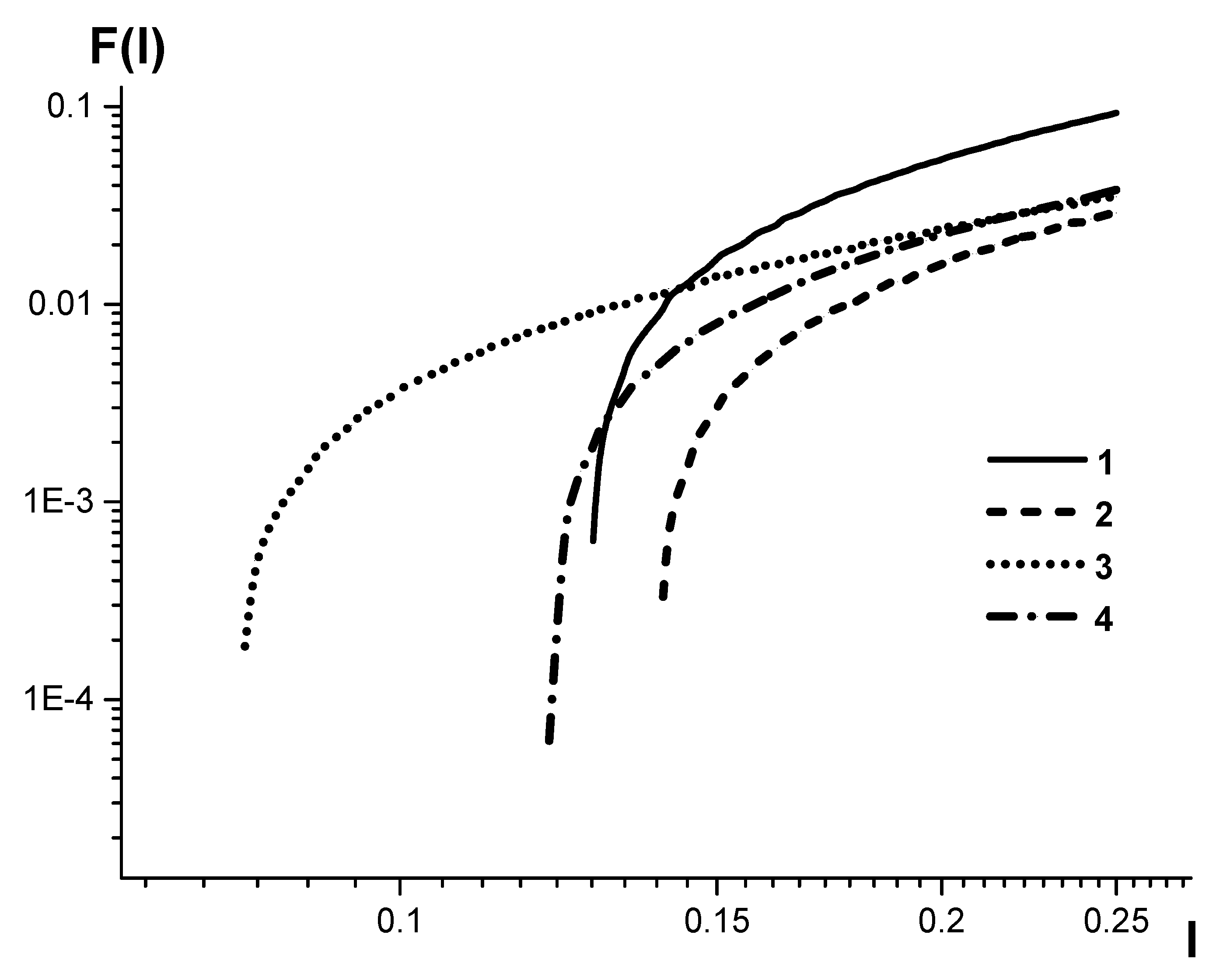
Figure 3 shows the calibrations to determine the carbon content in low- and medium-alloyed steels by standard samples UG0a-–UG9a, UG0e–UG9e, UG0k–UG9k, RG25a–RG31a for a SPAS-02 spectrometer (serial numbers № 22, 25, 26) and a SPAS-05 spectrometer (serial number № 18). The analytical carbon line CI 193.09 nm was used in this case. There are two types of calibration lines described: accounting for plasma background by the conventional algorithm (see above) and by adjusting using the suggested algorithm. The calibration curves were reduced to the same intensity range because the transmission coefficients of different devices may significantly vary. The corresponding coefficients were determined provided that the intensities of all devices were reduced to the same range of values $I-I_F$ in the area of low carbon concentrations.

It can be seen that in the area of relative carbon content lower than 0.15–0.3% (according to the particular device), the calibration-curve slope (2) begins to rise, which results in the several-fold increase of the RMS deviation of the determined concentration.

Simultaneously, the curves that were adjusted for the accurate background accounting in the area of low concentration have the form of straight lines with the slope of one. This is known to be optimal for emission-spectral-analysis calibration [22,23].

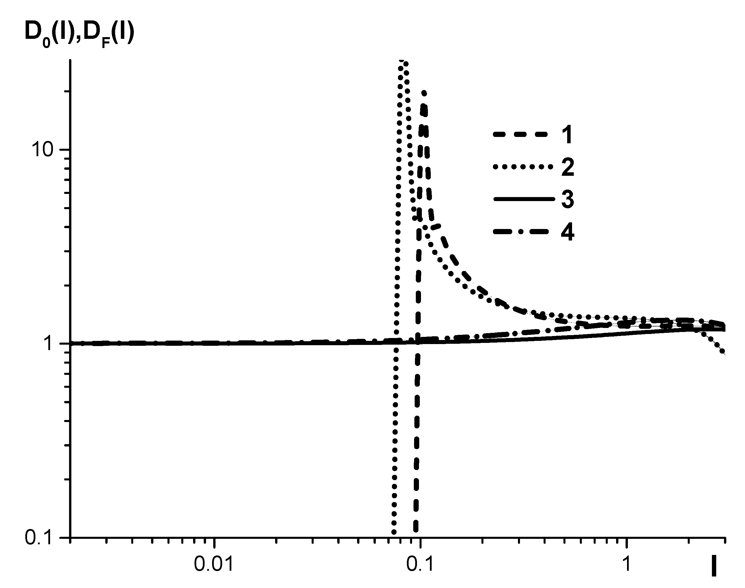
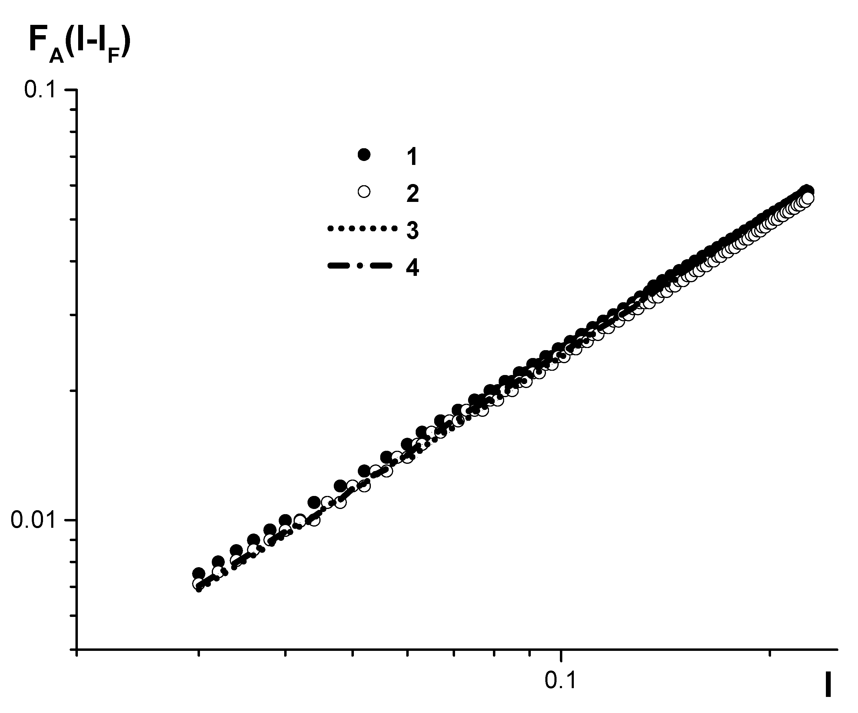
Figure 4 shows the dependences of slope calibrations $D_0(I)$, both unadjusted and adjusted for the accurate accounting of the plasma background $D_F(I)$ of the data in Figure 3 (SPAS-02 spectrometers, serial numbers №22, 26). Functions $D_0(I),$ $D_F(I)$ are determined by the following equations:

$$\begin{gathered} (I)=\frac{I}{F(I)}\frac{dF(I)}{dI}; \\ {D}_F(I)=\frac{I-I_F}{F_A(I-I_F)}\frac{d{F}_A(I-I_F)}{dI}. \end{gathered}$$

(29)

It can be seen that in the area of low relative intensities, the value $D_0(I)$ is more than an order higher than the optimal value equal to 1. If $I$ is further decreased, it becomes subzero, which lacks any physical meaning. That is why it is not shown in Figure 4 beyond this value area of $I$.

On the contrary, the slope $D_F(I)$ of the adjusted calibration curve in the whole area of $I>I_F$ is close to 1, which ensures a minimum RMS deviation while measuring concentrations.

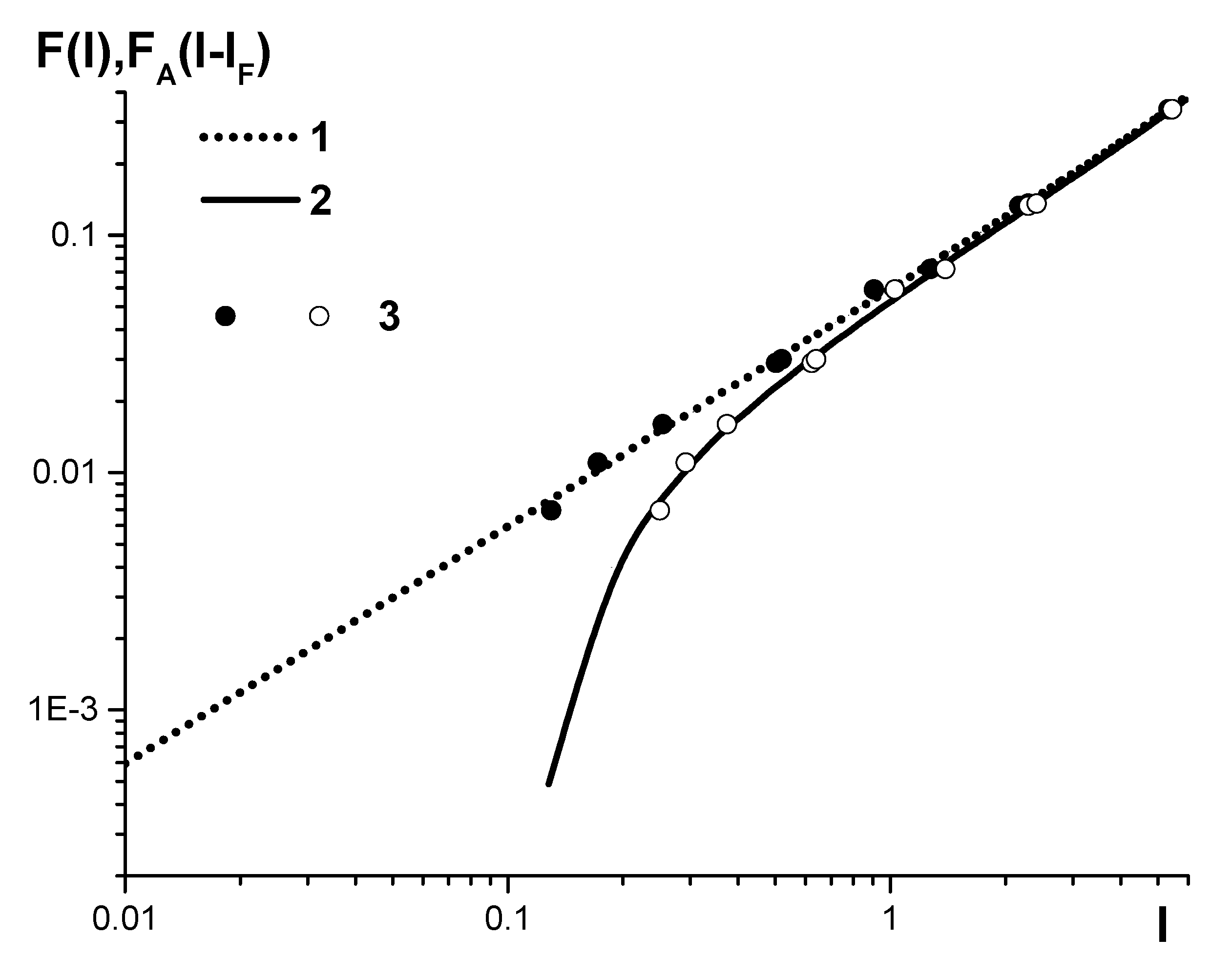
It should be noted that introducing coefficients $k$ before the relative intensity will reduce all the calibrations that were plotted with an accurate accounting of the plasma background to close curves related by a linear transformation (see Figure 5), despite the fact that:

• Various technologies for both spectrograph and generator (SPAS-02 and SPAS-05) manufacturing are utilized.
• Spectrometers have significantly different focus near the CI 193 nm line (the line width differs by up to twice);
• Various sets of standard samples (UG0a–UG9a, UG0e–UG9e, and UG0k–UG9k) are used.

This, in turn, creates opportunities for the primary calibration of spectrometers for specific types of alloys by a recalibration algorithm with linear-intensity transformation (see above), rather than by sets of dozens of standard samples.

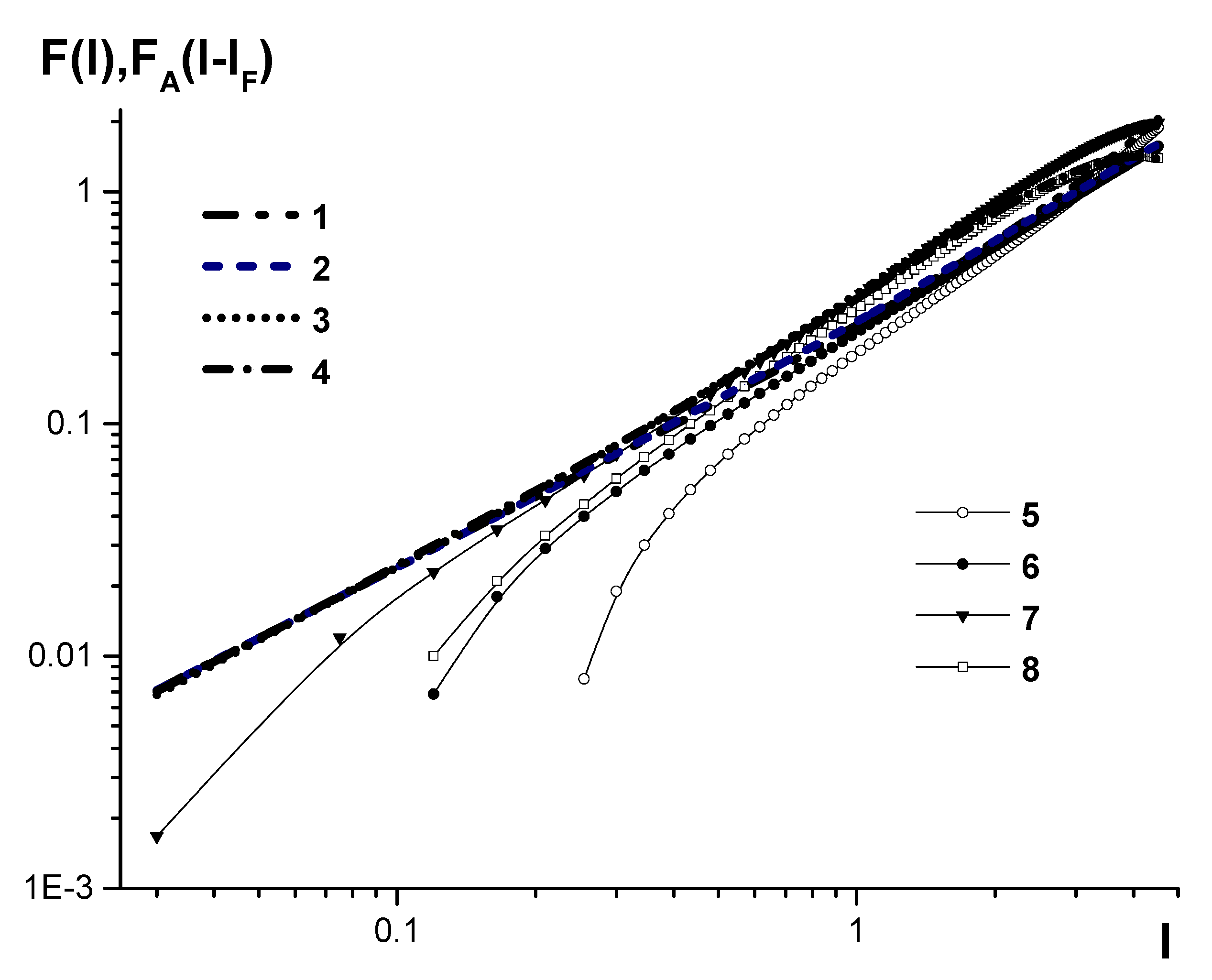
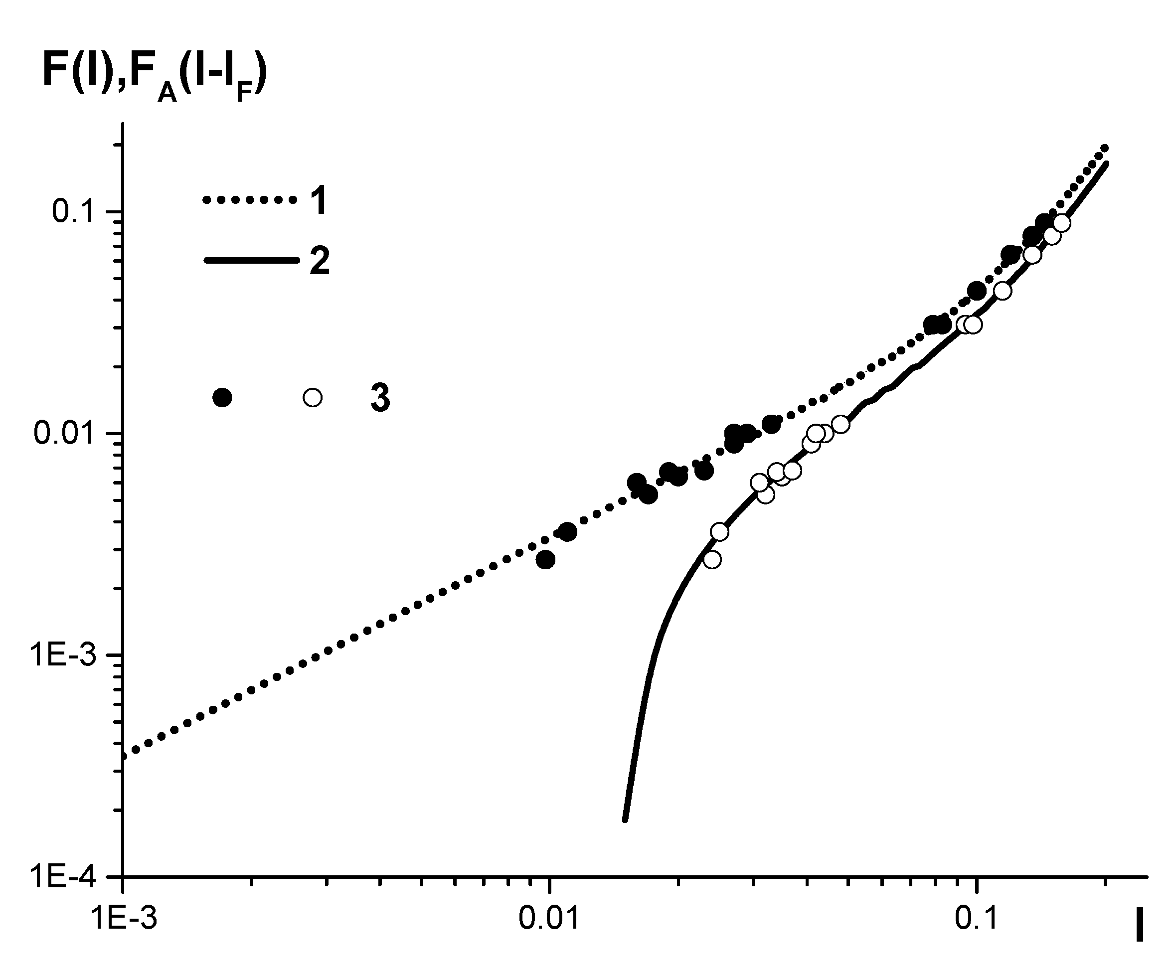
Figure 6 shows the calibration curves plotted by the conventional algorithm without accurate accounting for plasma background.

Figure 7 and Figure 8 show the calibration curves used to determine, for low- and medium-alloy steels, $P, Ti$, respectively, on SPAS-05 emission spectrometer, serial number №18, plotted with accurate accounting for plasma background by the conventional algorithm (see above) and adjusted by the developed algorithm. There are also the nameplate concentrations of the standard samples that were used. These data confirm the uniformity of the results obtained when determining carbon in steels.

5. Conclusions

Thus, the developed algorithm for the accurate accounting of plasma background radiation in the analytical-lines area enables:

• The significant reduction in RMS deviation while determining low impurity content in samples due to the optimal slope of the calibration curve in the area of low impurity concentrations;
• The scaling down of the detection limit of the sample impure element, in case plasma background radiation inaccuracy exceeds $3\mathsf{\sigma }$ of the background (where $\mathsf{\sigma }$ is the RMS deviation of the plasma background radiation from its average statistical value);
• The use, in commercial factory device calibration, of a maximum of two standard samples, rather than several dozens of them, to find linear-conversion parameters of the analytical-line intensity of a certain element by the recalibration algorithm.

We have clarified the conditions under which it is possible to apply conventional recalibration techniques (i.e., how the changes in a spectrometer parameters influence calibration curves during its continuous operation). Namely, this algorithm can be applied only in the case when the conditions for analytical-line intensity formation in plasma do not change while the device is in use, i.e., the spectrum-excitation-source parameters, inter-electrode distance, and in the case of utilizing specific plasma-forming gases, their purity, etc., stay unchanged. The algorithm is also applicable if there is a change in the transmission coefficient of the spectrometer and the parameters of analytical-line-intensity conversion into an electric signal.

Thus, special attention should be paid to the stability of the spectrum-excitation-source parameters when developing emission spectrometers.

It is defined that the linear relationship between the intensities measured by an emission-spectrometer recording system, when their parameters change, can only be implemented if the coefficients of transmission and intensity conversion into an electric signal by the recording system are independent of the analytical-line intensity. Otherwise, it is necessary to raise the degree of the polynomial relationship between these intensities, and therefore, to increase the number of standard samples required for recalibration.