
Controlling Remotely Operated Vehicles with Deterministic Artificial Intelligence


Abstract
:Featured Application
Abstract
1. Introduction
1.1. Proposed Innovations
- First-time development and presentation of deterministic artificial intelligence applied to yaw control of a remotely piloted submersible (the Seabotix vLBV 300 in this case): includes both self-awareness statements and newly presented parameterization of optimal learning.
- First instantiation of cubic polynomial autonomous trajectory generation supplied to deterministic self-awareness statements;
- Illustration of milli-degree tracking accuracy on the very first heading change of an aggressive shaped-square wave command, and an additional sixty percent (root mean square) error reduction by the third heading change of the square wave (illustrating the efficacy of optimal learning to eliminate startup transient behavior).
1.2. Manuscript Structure
2. Materials and Methods
2.1. Controller Architecture
2.2. System Dynamics
2.3. State Estimation
2.4. Trajectory Generation
2.5. Control Output
3. Results
4. Discussion
4.1. Findings and Their Implications
4.2. Recommendations for Future Research
Author Contributions
Funding
Data Availability Statement
Conflicts of Interest
Appendix A. MATLAB Code
dai_analysis.m
- clc
- clear
- close all
- log = ’20220128002145_10x_psi_step_30’;
- load([’scripts/’ ␣log␣ ’/’ log ’_ADAPTIVE_CTRL_STAT.mat’]);
- t = UNIX_timestamp - UNIX_timestamp(1);
- t_start = 0;
- t_end = 26;
- to_use = t > t_start & t < t_end;
- t = t(to_use);
- psi = polar_correct(PSI(to_use), -180, 180);
- psi_dot = PSI_DOT(to_use);
- psi_trajectory = polar_correct(PSI_TRAJ(to_use), -180, 180);
- setpoint = polar_correct(UC(to_use), -180, 180);
- first_start = 1.25;
- first_end = 6;
- first_step = t > first_start & t < first_end;
- first_step_info = stepinfo(psi(first_step), t(first_step) - first_start,
- ’RiseTimeLimits’, [0, 0.999], ’SettlingTimeThreshold’, 0.001)
- first_traj = psi_trajectory(first_step);
- first_traj(1) = 0;
- first_psi = psi(first_step);
- first_error = first_traj - first_psi;
- first_rms_error = sqrt(mean(first_error .^2))
- first_max_error = max(abs(first_error))
- last_start = 21.8;
- last_end = 26;
- last_step = t > last_start & t < last_end;
- last_step_info = stepinfo(psi(last_step), t(last_step) - last_start,
- ’RiseTimeLimits’, [0, 0.999], ’SettlingTimeThreshold’, 0.001)
- last_traj = psi_trajectory(last_step);
- last_psi = psi(last_step);
- last_error = last_traj - last_psi;
- last_rms_error = sqrt(mean(last_error .^2))
- last_max_error = max(abs(last_error))
- label_fontsize = 24;
- axis_fontsize = 18;
- linewidth = 1.25;
- ax = [t_start t_end 0 31];
- figure
- subplot(2, 1, 1)
- plot(t, psi, ’blue’, ’linewidth’, 2)
- title ’Yaw Step Response’
- ylabel(’$\psi$ (deg)’, ’Interpreter’, ’Latex’, ’FontSize’, axis_fontsize)
- xlabel(’Time (s)’)
- hold on
- plot(t, setpoint, ’red’, ’linewidth’, 2)
- plot(t, psi_trajectory, ’--c’, ’linewidth’, 2)
- legend({’$\psi$’, ’Setpoint’, ’Trajectory’}, ’Interpreter’, ’latex’, ’FontSize’, 22);
- set(gca, ’FontSize’, axis_fontsize)
- axis(ax);
- subplot(2, 1, 2)
- plot(t, psi_trajectory - psi, ’blue’, ’linewidth’, 2);
- title ’Yaw Error’
- ylabel(’$\psi$ Error (deg)’, ’Interpreter’, ’Latex’);
- xlabel ’Time (s)’
- set(gca, ’FontSize’, axis_fontsize)
- axis([t_start t_end -0.1 0.15])
- figure
- plot(psi, psi_dot)
- axis equal
Appendix B. C++ Code
Appendix B.1. adaptive_control.cpp
- /**
- * @author Shay Osler
- */
- #include <adaptive_control_version.h>
- #include <indirect_self_tuning_regulator.h>
- #include <dai.h>
- #include <matrix_utils.h>
- #include <state_estimator/state_estimator.h>
- #include <trajectory.h>
- #include <sinusoidal_trajectory.h>
- #include <cubic_trajectory.h>
- #include <SO_utils.h>
- #include <sno/logger.h>
- #include <sno/sno_macros.h>
- #include <sno/time_utils.h>
- #include <opencmd_defs.h>
- #include <opensea/ops.h>
- #include <opensea/gss_types/pcomms.h>
- #include <opensea/gss_types/effort.h>
- #include <opensea/gss_types/cmd.h>
- #include <opensea/gss_types/nav_solution.h>
- #include <lcm/lcm-cpp.hpp>
- #include <atomic>
- #include <chrono>
- #include <thread>
- ///////////////////////////////////////////////////////////////////////
- // Global Variables
- ///////////////////////////////////////////////////////////////////////
- namespace
- {
- /**
- * @brief Publish/subscribe interface
- */
- std::shared_ptr<gss::OPS> m_plcm;
- /**
- * @brief Channel to subscribe to nav solutions
- */
- std::string m_nav_channel = ″OPENINS_NAV_SOLUTION″;
- /**
- * @brief Channel to subscribe to setpoints on
- */
- std::string m_ctrl_cmd_channel = ″OPENCMD_CMD″;
- /**
- * @brief Channel to subscribe to opencmd efforts on
- */
- std::string m_effort_in_channel = ″OPENCMD_EFFORT″;
- /**
- * @brief Channel to publish effort commands on
- */
- std::string m_effort_out_channel = ″ADAPTIVE_CTRL_EFFORT″;
- /**
- * @brief Controller status channel
- */
- std::string m_status_channel = ″ADAPTIVE_CTRL_STAT″;
- /**
- * @brief Command channel
- */
- std::string m_cmd_channel = ″ADAPTIVE_CTRL_CMD″;
- /**
- * @brief Main thread sleep interval, ms
- */
- const std::chrono::milliseconds m_main_sleep_ms(50);
- /**
- * @brief Last received efforts
- */
- gss::types::Effort m_last_effort_rx;
- /**
- * @brief Last transmitted efforts
- */
- gss::types::Effort m_last_effort_tx;
- /**
- * @brief Indirect self tuning regulator
- */
- std::shared_ptr<ISTR> m_istr;
- static const size_t L = 15; // Number of parameters being estimated
- static const size_t N = 18; // Number of states
- static const size_t M = 6; // Control inputs
- /**
- * @brief Deterministic artificial intelligence controller
- */
- std::shared_ptr<DAI_controller<L, N, M>> m_dai;
- /**
- * @brief True if autopilot is enabled
- */
- bool m_enable_auto{false};
- /**
- * @brief True if DAI controller should be enabled
- */
- bool m_enable_dai{false};
- /**
- * @brief True if closed loop control should be used with DAI. If false then
- * DAI will only be used as a feed forward controller
- */
- bool m_enable_closed_loop_dai{false};
- /**
- * @brief True if ISTR controller should be enabled
- */
- bool m_enable_istr{false};
- /**
- * @brief Current controller setpoint
- */
- double m_setpoint{0};
- /**
- * @brief Time when the control move should be finished
- */
- double m_ctrl_tf{0};
- /**
- * @brief Kalman filter for estimating angular accelerations
- */
- State_estimator m_accel_estimator;
- /**
- * @brief Current trajectory to follow
- */
- std::shared_ptr<Trajectory> m_psi_trajectory;
- /**
- * @brief Last received nav solution
- */
- gss::types::Nav_solution m_last_soln;
- }
- ///////////////////////////////////////////////////////////////////////
- // Function Declarations
- ///////////////////////////////////////////////////////////////////////
- /**
- * @brief Initialize the indirect self tuning regulator
- */
- void Initialize_istr();
- /**
- * @brief Run the indirect self tuning regulator
- * @param Received nav solution
- */
- void Run_istr(const gss::types::Nav_solution* msg);
- /**
- * @brief Initialize the deterministic artifical intelligence controller
- */
- void Initialize_dai();
- /**
- * @brief Callback function for when controller commands are received
- * @param buf Received LCM buffer
- * @param channel Channel the message was received on
- * @param msg Command message
- */
- void On_ctrl_cmd_received(const gss::OPS::Receive_buffer&,
- const std::string&,
- const gss::types::Cmd* msg);
- /**
- * @brief Callback function for when vehicle nav solutions are received
- * @param buf Received LCM buffer
- * @param channel Channel the message was received on
- * @param msg Command message
- */
- void On_nav_received(const gss::OPS::Receive_buffer&,
- const std::string&,
- const gss::types::Nav_solution* msg);
- /**
- * @brief Callback function for when effort commands are received
- * @param buf Received LCM buffer
- * @param channel Channel the message was received on
- * @param msg Command message
- */
- void On_effort_received(const gss::OPS::Receive_buffer&,
- const std::string&,
- const gss::types::Effort* msg);
- /**
- * @brief Generate a trajectory from the current position to the specified position
- * and velocity
- * @param xf Final Position
- * @param vf Final velocity
- * @return Trajectory
- */
- std::shared_ptr<Trajectory> Generate_trajectory(const double xf,
- const double vf =0 );
- ///////////////////////////////////////////////////////////////////////
- // Function Definitions
- ///////////////////////////////////////////////////////////////////////
- void Initialize_istr()
- {
- // Mark last received efforts as invalid
- m_last_effort_rx.time_unix_sec = −1;
- // Desired TF:
- // 0.1761q
- // -----------------------
- // (q^2 + 1.223q + 0.3743)
- // Eigen::Matrix<double, ISTR::N, 1> Am{1.223, 0.3743};
- Eigen::Matrix<double, ISTR::N, 1> Am{-1.3205, 0.4966};
- Eigen::Matrix<double, ISTR::M+1, 1> Bm{8.0186, 3.1818};
- double a0 = 0;
- Eigen::Matrix<double, ISTR::N+ISTR::M+1, 1> theta0{0, 0, 0.01, 0.2};
- Eigen::Matrix<double, ISTR::N+ISTR::M+1, ISTR::N+ISTR::M+1> P0{{100, 0, 0, 0},
- {0, 100, 0, 0},
- {0, 0, 1, 0},
- {0, 0, 0, 1}};
- m_istr = std::make_shared<ISTR>(Am, Bm, a0, theta0, P0);
- }
- ///////////////////////////////////////////////////////////////////////
- void Run_istr(const gss::nav_solution_t* msg)
- {
- // Check that nav is valid
- if(!msg->attitude_ok)
- {
- return;
- }
- if(!m_istr)
- {
- return;
- }
- // run every nth time
- static size_t count = 0;
- if( (count++
- {
- return;
- }
- // Get controller output
- double y = msg->attitude_dot[2];
- const auto [effort, theta_hat] = m_istr->Get_control_output(y,
- m_setpoint,
- m_last_effort_tx.effort_psi);
- {}
- // If we’re in closed loop mode, publish
- if(m_enable_auto
- && m_enable_istr
- && m_last_effort_rx.time_unix_sec > 0)
- {
- gss::effort_t effort_cmd = m_last_effort_rx;
- double effort_out = effort;
- double max_effort = 50;
- double min_effort = -max_effort;
- if(effort_out > max_effort)
- {
- effort_out = max_effort;
- }
- else if(effort_out < min_effort)
- {
- effort_out = min_effort;
- }
- effort_cmd.effort_psi = effort_out;
- m_plcm->Publish(m_effort_out_channel, &effort_cmd);
- m_last_effort_tx = effort_cmd;
- }
- gss::pcomms_t stat;
- static uint32_t count_publish = 0;
- stat.time_unix_sec = so::Time_utils::Unix_time();
- stat.count_publish = count_publish++;
- stat.analogs.push_back({″A1″, theta_hat[0]});
- stat.analogs.push_back({″A2″, theta_hat[1]});
- stat.analogs.push_back({″B0″, theta_hat[2]});
- stat.analogs.push_back({″B1″, theta_hat[3]});
- stat.analogs.push_back({″UC″, m_setpoint});
- stat.analogs.push_back({″U″, effort});
- stat.analogs.push_back({″Y″, y});
- stat.digitals.push_back({″AUTO_DEPTH_ENABLE″, m_enable_auto});
- stat.num_analogs = stat.analogs.size();
- stat.num_digitals = stat.digitals.size();
- stat.num_messages = stat.messages.size();
- m_plcm->Publish(m_status_channel, &stat);
- }
- ///////////////////////////////////////////////////////////////////////
- void Initialize_dai()
- {
- // Initialize acceleration estimator
- m_accel_estimator.Initialize(so::Time_utils::Unix_time(),
- State_estimator::Kf_type::MatrixN1::Zero(),
- 360 * State_estimator::Kf_type::MatrixNN::Identity());
- // Mark last received efforts as invalid
- m_last_effort_rx.time_unix_sec = −1;
- Eigen::Matrix<double, L, 1> theta0 = Eigen::Matrix<double, L, 1>::Ones();
- // theta0(15) = −1;
- Eigen::Matrix<double, L, L> P0 = Eigen::Matrix<double, L, L>::Identity() * 100;
- m_dai = std::make_shared<DAI_controller<L, N, M>>(theta0, P0);
- }
- ///////////////////////////////////////////////////////////////////////
- void On_ctrl_cmd_received(const gss::OPS::Receive_buffer&,
- const std::string&,
- const gss::types::Cmd* msg)
- {
- m_enable_auto = msg->enable_state_psi == Opencmd_defs::EEnable_Auto;
- const double min_change = 1;
- if( std::fabs(msg->cmd_psi - m_setpoint) > min_change
- && m_last_soln.unix_time > 0)
- {
- m_psi_trajectory = Generate_trajectory(msg->cmd_psi);
- m_setpoint = msg->cmd_psi;
- }
- }
- ///////////////////////////////////////////////////////////////////////
- void On_nav_received(const gss::OPS::Receive_buffer&,
- const std::string&,
- const gss::types::Nav_solution* msg)
- {
- m_last_soln = *msg;
- // Check that nav is valid
- if(!msg->attitude_ok)
- {
- return;
- }
- if(!m_dai)
- {
- return;
- }
- // Current state
- Eigen::Matrix<double, 18, 1> Y =
- {
- msg->absolute_position[0], // TODO: what is the correct ″X″ state? Meters
- North of setpoint? Meters body frame forward of setpoint?
- msg->absolute_position[1], // TODO: what is the correct ″Y″ state? Meters
- East of setpoint? Meters body frame right of setpoint?
- msg->absolute_position[2],
- msg->attitude[0],
- msg->attitude[1],
- msg->attitude[2],
- msg->relative_position_dot[0],
- msg->relative_position_dot[1],
- msg->relative_position_dot[2],
- msg->attitude_dot[0],
- msg->attitude_dot[1],
- msg->attitude_dot[2],
- msg->relative_acceleration[0],
- msg->relative_acceleration[1],
- msg->relative_acceleration[2],
- msg->attitude_acceleration[0], // TODO: estimate this when not using simulator
- msg->attitude_acceleration[1], // TODO: estimate this when not using simulator
- msg->attitude_acceleration[2] // TODO: estimate this when not using simulator
- };
- // Get trajectory
- // TODO: move trajectory into DAI?
- // If we’re in closed loop dai mode continually update the trajectory to move
- // us to the setpoint
- // if(m_enable_closed_loop_dai)
- // {
- // m_psi_trajectory = Generate_trajectory(m_setpoint);
- // }
- auto d = Y;
- double psi_traj = 0;
- double psi_dot_traj = 0;
- double psi_ddot_traj = 0;
- if(m_psi_trajectory)
- {
- // Calculate the current state prescribed by the trajectory
- std::tie(psi_traj, psi_dot_traj, psi_ddot_traj) =
- m_psi_trajectory->Get_states(so::Time_utils::Unix_time());
- d(5) = psi_traj;
- d(11) = psi_dot_traj;
- d(17) = psi_ddot_traj;
- if(m_enable_closed_loop_dai)
- {
- // TODO: Try just calculating a psi trajectory once when the setpoint
- // changes. Then pick a fixed time window T, and calculate a ″full″ (i.e.,
- // psi, psi_dot, psi_ddot) trajectory from the current position to the
- // position on the main trajectory at time t + T, and use that for the control
- // that way we always track the original trajectory
- static const double T = 0.25;
- const auto [psi_traj_now, psi_dot_traj_now, psi_ddot_traj_now] =
- m_psi_trajectory->Get_states(so::Time_utils::Unix_time() + T);{}
- auto now_traj =
- std::make_shared<Cubic_trajectory>(so::Time_utils::Unix_time(),
- m_last_soln.attitude[2],
- m_last_soln.attitude_dot[2],
- psi_traj_now,
- psi_dot_traj_now,
- 0.25,
- true);
- const auto[psi_d, psi_dot_d, psi_ddot_d] = now_traj->Get_states(so::Time_utils::
- Unix_time());{}
- d(5) = psi_d;
- d(11) = psi_dot_d;
- d(17) = psi_ddot_d;
- }
- }
- // Estimate accels
- Eigen::Matrix<double, 6, 1> z{msg->attitude[0],
- msg->attitude_dot[0],
- msg->attitude[1],
- msg->attitude_dot[1],
- msg->attitude[2],
- msg->attitude_dot[2]};
- double r = 1e − 3;
- Eigen::Matrix<double, 6, 6> R = Eigen::Matrix<double, 6, 6>::Zero();
- R(0,0) = r;
- R(1,1) = r;
- R(2,2) = r;
- R(3,3) = r;
- R(4,4) = r;
- R(5,5) = r;
- Measurement<6> m(″ins″,
- msg->unix_time,
- z,
- {State_estimator_defs::Phi,
- State_estimator_defs::Phi_dot,
- State_estimator_defs::Theta,
- State_estimator_defs::Theta_dot,
- State_estimator_defs::Psi,
- State_estimator_defs::Psi_dot},
- R);
- auto attitude_hat = m_accel_estimator.Get_state_estimates();
- Eigen::Matrix<double, 3, 1> ctrl
- {
- 0,
- 0,
- d(17) - attitude_hat[State_estimator_defs::Psi_accel]
- };
- m_accel_estimator.Update(ctrl, m);
- attitude_hat = m_accel_estimator.Get_state_estimates();
- Y(15) = attitude_hat[State_estimator_defs::Phi_accel];
- Y(16) = attitude_hat[State_estimator_defs::Theta_accel];
- Y(17) = attitude_hat[State_estimator_defs::Psi_accel];
- static double t_last_psi = −1;
- static double last_psi_dot = 0;
- double psi_accel_num_deriv = 0;
- if(t_last_psi > 0)
- {
- double d_psi_dot = msg->attitude_dot[2] - last_psi_dot;
- double dt = so::Time_utils::Unix_time() - t_last_psi;
- psi_accel_num_deriv = d_psi_dot / dt;
- }
- t_last_psi = so::Time_utils::Unix_time();
- last_psi_dot = msg->attitude_dot[2];
- // Most recent effort commands
- Eigen::Matrix<double, 6, 1> u =
- {
- m_last_effort_tx.effort_x,
- m_last_effort_tx.effort_y,
- m_last_effort_tx.effort_z,
- m_last_effort_tx.effort_phi,
- m_last_effort_tx.effort_theta,
- m_last_effort_tx.effort_psi,
- };
- // Current setpoints
- Eigen::Matrix<double, 6, 1> u_c
- {
- 0,
- 0,
- 0,
- 0,
- 0,
- m_setpoint
- };
- // Get controller output
- const auto [effort, theta_hat] = m_dai->Get_control_output(Y, d, u);
- {}
- double psi_effort = effort(5);
- // If we’re in closed loop mode, publish controller efforts
- if(m_enable_auto && m_last_effort_rx.time_unix_sec > 0 && m_enable_dai)
- {
- gss::effort_t effort_cmd = m_last_effort_rx;
- double psi_effort_out = psi_effort;
- double max_effort = 50;
- double min_effort = -max_effort;
- if(psi_effort_out > max_effort)
- {
- psi_effort_out = max_effort;
- }
- else if(psi_effort_out < min_effort)
- {
- psi_effort_out = min_effort;
- }
- effort_cmd.effort_psi = psi_effort_out;
- m_plcm->Publish(m_effort_out_channel, &effort_cmd);
- m_last_effort_tx = effort_cmd;
- }
- // Extract parameter estimates
- double I_zx = theta_hat(0);
- double N_p_dot = theta_hat(1);
- double I_zy = theta_hat(2);
- double N_q_dot = theta_hat(3);
- double I_z = theta_hat(4);
- double N_r_dot = theta_hat(5);
- double N_u_dot = theta_hat(6);
- double N_v_dot = theta_hat(7);
- double N_w_dot = theta_hat(8);
- double g_y_m = theta_hat(9);
- double g_x_m = theta_hat(10);
- double V_b_y_rho = theta_hat(11);
- double V_b_x_rho = theta_hat(12);
- double N_r = theta_hat(13);
- double N_rr = theta_hat(14);
- double A0 = 21.3333333333333; //theta_hat(15);
- double A1 = 0.133333333333333; //theta_hat(16);
- gss::pcomms_t stat;
- static uint32_t count_publish = 0;
- stat.time_unix_sec = so::Time_utils::Unix_time();
- stat.count_publish = count_publish++;
- // Parameter estimates
- stat.analogs.push_back({″I_ZX″ , I_zx });
- stat.analogs.push_back({″N_P_DOT″ , N_p_dot });
- stat.analogs.push_back({″I_ZY″ , I_zy });
- stat.analogs.push_back({″N_Q_DOT″ , N_q_dot });
- stat.analogs.push_back({″I_Z″ , I_z });
- stat.analogs.push_back({″N_R_DOT″ , N_r_dot });
- stat.analogs.push_back({″N_U_DOT″ , N_u_dot });
- stat.analogs.push_back({″N_V_DOT″ , N_v_dot });
- stat.analogs.push_back({″N_W_DOT″ , N_w_dot });
- stat.analogs.push_back({″G_Y*M″ , g_y_m });
- stat.analogs.push_back({″G_X*M″ , g_x_m });
- stat.analogs.push_back({″V*B_Y*RHO″, V_b_y_rho});
- stat.analogs.push_back({″V*B_X*RHO″, V_b_x_rho});
- stat.analogs.push_back({″N_R″ , N_r });
- stat.analogs.push_back({″N_RR″ , N_rr });
- stat.analogs.push_back({″A0″ , A0 });
- stat.analogs.push_back({″A1″ , A1 });
- // Current states
- stat.analogs.push_back({″X″, msg->absolute_position[0]}); // TODO: what is the
- correct ″X″ state? Meters North of setpoint?
- stat.analogs.push_back({″Y″, msg->absolute_position[1]}); // TODO: what is the
- correct ″Y″ state? Meters East of setpoint?
- stat.analogs.push_back({″Z″, msg->absolute_position[2]});
- stat.analogs.push_back({″PHI″, msg->attitude[0]});
- stat.analogs.push_back({″THETA″, msg->attitude[1]});
- stat.analogs.push_back({″PSI″, msg->attitude[2]});
- stat.analogs.push_back({″X_DOT″, msg->relative_position_dot[0]});
- stat.analogs.push_back({″Y_DOT″, msg->relative_position_dot[1]});
- stat.analogs.push_back({″Z_DOT″, msg->relative_position_dot[2]});
- stat.analogs.push_back({″PHI_DOT″, msg->attitude_dot[0]});
- stat.analogs.push_back({″THETA_DOT″, msg->attitude_dot[1]});
- stat.analogs.push_back({″PSI_DOT″, msg->attitude_dot[2]});
- stat.analogs.push_back({″X_ACCEL″, msg->relative_acceleration[0]});
- stat.analogs.push_back({″Y_ACCEL″, msg->relative_acceleration[1]});
- stat.analogs.push_back({″Z_ACCEL″, msg->relative_acceleration[2]});
- stat.analogs.push_back({″PHI_ACCEL″, msg->attitude_acceleration[0]});
- stat.analogs.push_back({″THETA_ACCEL″, msg->attitude_acceleration[1]});
- stat.analogs.push_back({″PSI_ACCEL″, msg->attitude_acceleration[2]});
- // Estimates for attitude
- stat.analogs.push_back({″PHI^″, attitude_hat[State_estimator_defs::Phi]});
- stat.analogs.push_back({″THETA^″, attitude_hat[State_estimator_defs::Theta]});
- stat.analogs.push_back({″PSI^″, attitude_hat[State_estimator_defs::Psi]});
- stat.analogs.push_back({″PHI_DOT^″, attitude_hat[State_estimator_defs::Phi_dot]});
- stat.analogs.push_back({″THETA_DOT^″,
- attitude_hat[State_estimator_defs::Theta_dot]});
- stat.analogs.push_back({″PSI_DOT^″,
- attitude_hat[State_estimator_defs::Psi_dot]});
- stat.analogs.push_back({″PHI_ACCEL^″,
- attitude_hat[State_estimator_defs::Phi_accel]});
- stat.analogs.push_back({″THETA_ACCEL^″,
- attitude_hat[State_estimator_defs::Theta_accel]});
- stat.analogs.push_back({″PSI_ACCEL^″,
- attitude_hat[State_estimator_defs::Psi_accel]});
- stat.analogs.push_back({″PSI_ACCEL*″, psi_accel_num_deriv});
- // Trajectory
- if(m_psi_trajectory)
- {
- stat.analogs.push_back({″PSI_TRAJ″, psi_traj});
- stat.analogs.push_back({″PSI_DOT_TRAJ″, psi_dot_traj});
- stat.analogs.push_back({″PSI_ACCEL_TRAJ″, psi_ddot_traj});
- stat.analogs.push_back({″PSI_D″, d(5)});
- stat.analogs.push_back({″PSI_DOT_D″, d(11)});
- stat.analogs.push_back({″PSI_ACCEL_D″, d(17)});
- }
- // Setpoints/efforts
- stat.analogs.push_back({″UC″, m_setpoint});
- stat.analogs.push_back({″U_PSI″, psi_effort});
- stat.analogs.push_back({″PSI_DOT″, msg->attitude_dot[2]});
- stat.digitals.push_back({″AUTO_ENABLED″, m_enable_auto});
- stat.digitals.push_back({″DAI_ENABLED″, m_enable_dai});
- stat.digitals.push_back({″DAI_CLOSED_LOOP_ENABLED″, m_enable_closed_loop_dai});
- stat.digitals.push_back({″ISTR_ENABLED″, m_enable_istr});
- stat.num_analogs = stat.analogs.size();
- stat.num_digitals = stat.digitals.size();
- stat.num_messages = stat.messages.size();
- m_plcm->Publish(m_status_channel, &stat);
- }
- ///////////////////////////////////////////////////////////////////////
- void On_effort_received(const gss::OPS::Receive_buffer&,
- const std::string&,
- const gss::types::Effort* msg)
- {
- // Cache last received efforts
- m_last_effort_rx = *msg;
- // If closed loop isn’t enabled, publish effort out directly
- if(!m_enable_auto ||
- !(m_enable_dai || m_enable_istr))
- {
- m_plcm->Publish(m_effort_out_channel, msg);
- m_last_effort_tx = *msg;
- }
- }
- ///////////////////////////////////////////////////////////////////////
- std::shared_ptr<Trajectory> Generate_trajectory(const double xf,
- const double vf)
- {
- const double desired_rate = 3;
- const double dx = std::fabs(SO_utils::Angle_diff(m_last_soln.attitude[2],
- xf));
- double traj_dt = dx < 5 ? dx / desired_rate
- : 5/desired_rate + (dx - 5) * 0.03;
- const double min_dt = 0.15;//0.3;
- if(traj_dt < min_dt)
- {
- traj_dt = min_dt;
- }
- // auto traj =
- // std::make_shared<Sinusoidal_trajectory>(so::Time_utils::Unix_time(),
- // m_last_soln.attitude[2],
- // xf,
- // traj_dt,
- // true);
- auto traj =
- std::make_shared<Cubic_trajectory>(so::Time_utils::Unix_time(),
- m_last_soln.attitude[2],
- m_last_soln.attitude_dot[2],
- xf,
- vf,
- traj_dt,
- true);
- m_ctrl_tf = so::Time_utils::Unix_time() + traj_dt;
- return traj;
- }
- ///////////////////////////////////////////////////////////////////////
- void On_cmd_received(const gss::OPS::Receive_buffer&,
- const std::string&,
- const gss::types::Pcomms* msg)
- {
- for(const auto& dig : msg->digitals)
- {
- if(dig.name == ″ENABLE_DAI″)
- {
- m_enable_dai = dig.value;
- if(dig.value)
- {
- m_enable_istr = false;
- }
- }
- else if(dig.name == ″ENABLE_CLOSED_LOOP_DAI″)
- {
- m_enable_closed_loop_dai = dig.value;
- }
- }
- }
- ///////////////////////////////////////////////////////////////////////
- /**
- * Main
- */
- int main(int argc, char *argv[])
- {
- so::Log_msg(so::Logger::Info,
- ″Adaptive control application version %s″,
- SNO_XSTRINGIFY(APPLICATION_VERSION_FULL));
- //////////////////////////////////////////////////////
- // Initialize Logging
- so::Logger::Set_logging_level(so::Logger::Debug);
- //////////////////////////////////////////////////////
- // Set Application Defaults
- std::string logging_level = ″Debug″;
- std::string lcm_url;
- //////////////////////////////////////////////////////
- // TODO: Set up the program options
- lcm_url = ″udpm://239.255.76.67:7665?ttl=0″;
- //////////////////////////////////////////////////////
- // Print application info
- so::Log_msg(so::Logger::Info,
- ″Pub/sub URL %s″,
- lcm_url.c_str());
- so::Log_msg(so::Logger::Info,
- ″Subscribing to nav solutions on channel %s″,
- m_nav_channel.c_str());
- so::Log_msg(so::Logger::Info,
- ″Subscribing to controller setpoints on channel %s″,
- m_ctrl_cmd_channel.c_str());
- so::Log_msg(so::Logger::Info,
- ″Subscribing to efforts on channel %s″,
- m_effort_in_channel.c_str());
- so::Log_msg(so::Logger::Info,
- ″Subscribing to commands on channel %s″,
- m_cmd_channel.c_str());
- so::Log_msg(so::Logger::Info,
- ″Publishing efforts on channel %s″,
- m_effort_out_channel.c_str());
- so::Log_msg(so::Logger::Info,
- ″Publishing status on channel %s″,
- m_status_channel.c_str());
- //////////////////////////////////////////////////////
- // Initialize LCM
- try
- {
- m_plcm = std::make_shared<gss::OPS>(lcm_url);
- }
- catch(const std::exception& e)
- {
- so::Log_msg(so::Logger::Fatal,
- ″Failed to initialize pub/sub interface: %s″,
- e.what());
- }
- // Subscribe
- m_plcm->Subscribe(m_ctrl_cmd_channel,
- &On_ctrl_cmd_received);
- m_plcm->Subscribe(m_nav_channel,
- &On_nav_received);
- m_plcm->Subscribe(m_effort_in_channel,
- &On_effort_received);
- m_plcm->Subscribe(m_cmd_channel,
- &On_cmd_received);
- //////////////////////////////////////////////////////
- // Set the signal handler for SIGINT
- //TODO
- //////////////////////////////////////////////////////
- // Initialize controllers
- try
- {
- Initialize_istr();
- Initialize_dai();
- }
- catch(const std::exception& e)
- {
- so::Log_msg(so::Logger::Fatal,
- ″Failed to initialize controller: %s″,
- e.what());
- return EXIT_FAILURE;
- }
- //////////////////////////////////////////////////////
- // Main loop
- while(true)
- {
- // Handle received messages
- while(m_plcm->Handle(1.0)) {}
- }
- return EXIT_SUCCESS;
- }
Appendix B.2. dai.h
- #ifndef DAI_CONTROLLER_H
- #define DAI_CONTROLLER_H
- #include <rls.h>
- #include <units.h>
- #include <sno/logger.h>
- #include <sno/so_exception.h>
- #include <eigen3/Eigen/Dense>
- #include <eigen3/unsupported/Eigen/Polynomials>
- #include <tuple>
- #include <vector>
- namespace
- {
- /**
- * @brief Find solution to polynomial of the form
- * f = a1 * u * |u| + a0 * u
- * @param a0 Coefficient
- * @param a1 Coefficient
- * @param f Desired force
- * @return Effort required for that force
- */
- // TODO: I’m pretty sure this is wrong
- // Relies on some assumptions that aren’t necessarily true
- double force_to_effort(const double a0,
- const double a1,
- const double f)
- {
- // Trivial cases
- // If force is approximately 0, effort is approximately 0
- if(std::fabs(f) < 1e − 9)
- {
- return 0;
- }
- // If quadratic coefficient is approximately 0, then just ignore it
- if(std::fabs(a1) < 1e − 9)
- {
- return f / a0;
- }
- // Solve quadratic w/ absolute value:
- double u = 0;
- if(a1 > 0)
- {
- if(f > 0)
- {// u will be positive
- // a0^2 > 0, a1 > 0, f > 0 -> radicand must be positive
- double radicand = a0 * a0 + 4 * a1 * f;
- // 2 solutions:
- // u1 = (−a0 + std::sqrt(radicand)) / (2 * a1)
- // u2 = (−a0 - std::sqrt(radicand)) / (2 * a1)
- // radicand will always be > a0^2, so sqrt(radicand) will always be greater
- // than a0, so for a positive u the solution will be:
- u = (−a0 + std::sqrt(radicand)) / (2 * a1);
- }
- else
- { // u will be negative
- // a0^2 > 0, a1 > 0, f < 0 -> radicand must be positive
- double radicand = a0 * a0 - 4 * a1 * f;
- // 2 solutions:
- // u1 = (−a0 + std::sqrt(radicand)) / (−2 * a1)
- // u2 = (−a0 − std::sqrt(radicand)) / (−2 * a1)
- // radicand will always be > a0^2, so sqrt(radicand) will always be greater
- // than a0, so for a negative u the solution will be
- u = (−a0 + std::sqrt(radicand)) / (−2 * a1);
- }
- }
- else
- { // a1 < 0
- if(f > 0)
- {// u will be negative
- // a0^2 > 0, a1 < 0, f > 0 -> radicand must be positive
- double radicand = a0 * a0 − 4 * a1 * f;
- // As above, solution for a negative u will be:
- u = (−a0 + std::sqrt(radicand)) / (−2 * a1);
- }
- else
- { // u will be positive
- // a0^2 > 0, a1 < 0, f < 0 -> radicand must be positive
- double radicand = a0 * a0 + 4 * a1 * f;
- // As above, the solution for a positive u will be
- u = (−a0 + std::sqrt(radicand)) / (2 * a1);
- }
- }
- return u;
- }
- }
- /**
- * @brief The DAI_controller class
- * @tparam L Number of parameters in the dynamics model to estimate
- * @tparam N Number of system states
- * @tparam M Number of control inputs
- */
- template<size_t L, size_t N, size_t M = N>
- class DAI_controller
- {
- public:
- typedef Eigen::Matrix<double, L, 1> MatrixL1;
- typedef Eigen::Matrix<double, L, L> MatrixLL;
- typedef Eigen::Matrix<double, N, N> MatrixNN;
- typedef Eigen::Matrix<double, 1, N> Matrix1N;
- typedef Eigen::Matrix<double, N, 1> MatrixN1;
- typedef Eigen::Matrix<double, N, M> MatrixNM;
- typedef Eigen::Matrix<double, M, 1> MatrixM1;
- DAI_controller(const MatrixL1& theta0,
- const MatrixLL& P0)
- :
- m_theta_hat(theta0),
- m_rls(theta0, P0)
- {
- }
- /**
- * @brief Get the control output
- * @param Y Current system state:
- * [x y z phi theta psi u v w p q r u_dot v_dot w_dot p_dot q_dot r_dot]’
- * @param d Current desired states (setpoints):
- * [x y z phi theta psi u v w p q r u_dot v_dot w_dot p_dot q_dot r_dot]’
- * @param u_t Current effort commands:
- * [u_x u_y u_z u_phi u_theta u_psi]’
- * @return Control output and current parameter estimates:
- * [u_x u_y u_z u_phi u_theta u_psi]’
- *
- */
- std::tuple<MatrixM1, MatrixL1> Get_control_output(const MatrixN1& Y,
- const MatrixN1& d,
- const MatrixM1& u_t)
- {
- // Get states out of Y
- // TODO: make structured bindings work with eigen matrices
- // TODO: transform Y from inertial to body where necessary?
- double x = Y(0);
- double y = Y(1);
- double z = Y(2);
- double phi = Units::Deg_to_rad(Y(3));
- double theta = Units::Deg_to_rad(Y(4));
- double psi = Units::Deg_to_rad(Y(5));
- double u = Y(6);
- double v = Y(7);
- double w = Y(8);
- double p = Units::Deg_to_rad(Y(9));
- double q = Units::Deg_to_rad(Y(10));
- double r = Units::Deg_to_rad(Y(11));
- double u_dot = Y(12);
- double v_dot = Y(13);
- double w_dot = Y(14);
- double p_dot = Units::Deg_to_rad(Y(15));
- double q_dot = Units::Deg_to_rad(Y(16));
- double r_dot = Units::Deg_to_rad(Y(17));
- // Get current effort commands out of u_t
- double u_x = u_t(0);
- double u_y = u_t(1);
- double u_z = u_t(2);
- double u_phi = u_t(3);
- double u_theta = u_t(4);
- double u_psi = u_t(5);
- // Update estimates for model parameters
- // Model is of form a*u = PHI * THETA -> u = PHI * THETA / a
- // Put into regression form: Y = PHI * THETA
- // PHI = …
- // [−p_dot p_dot −q_dot q_dot r_dot r_dot u_dot v_dot w_dot …
- // (-g*sin(theta) - u_dot) (v_dot - g*cos(theta)*sin(phi)) g*sin(theta)
- g*cos(theta)*sin(phi)…
- // -r -abs(r)*r];
- // THETA = …
- // [I_zx N_p_dot I_zy N_q_dot I_z N_r_dot N_u_dot N_v_dot N_w_dot g_y*m g_x*m
- V*b_y*rho V*b_x*rho N_r N_rr].’;
- ␣␣␣␣//␣Build␣PHI
- ␣␣␣␣static␣const␣double␣g␣=␣9.8;␣//␣Gravity
- ␣␣␣␣Eigen::Matrix<double,␣1,␣L>␣PHI␣=
- ␣␣␣␣{
- ␣␣␣␣␣␣//␣System␣states
- ␣␣␣␣␣␣−p_dot,
- ␣␣␣␣␣␣p_dot,
- ␣␣␣␣␣␣−q_dot,
- ␣␣␣␣␣␣q_dot,
- ␣␣␣␣␣␣r_dot,
- ␣␣␣␣␣␣r_dot,
- ␣␣␣␣␣␣u_dot,
- ␣␣␣␣␣␣v_dot,
- ␣␣␣␣␣␣w_dot,
- ␣␣␣␣␣␣(-g␣*␣std::sin(theta)␣-␣u_dot),
- ␣␣␣␣␣␣(v_dot␣-␣g␣*␣std::cos(theta)␣*␣std::sin(phi)),
- ␣␣␣␣␣␣g␣*␣std::sin(theta),
- ␣␣␣␣␣␣g␣*␣std::cos(theta)␣*␣std::sin(phi),
- ␣␣␣␣␣␣-r,
- ␣␣␣␣␣␣-std::abs(r)␣*␣r,
- ␣
- ␣␣␣␣␣␣//␣Current␣control␣inputs
- //␣␣␣␣␣␣-u_psi,
- //␣␣␣␣␣␣-std::abs(u_psi)␣*␣u_psi
- ␣␣␣␣};
- ␣
- ␣␣␣␣//␣Force␣to␣efforce␣conversion␣parameters
- //␣␣␣␣double␣A1␣=␣0.133333333333333;
- //␣␣␣␣double␣A0␣=␣21.3333333333333;
- ␣␣␣␣double␣A1␣=␣0;
- ␣␣␣␣double␣A0␣=␣1;
- ␣
- ␣␣␣␣//␣Estimate␣parameters
- ␣␣␣␣double␣force␣=␣A1␣*␣u_psi␣*␣std::abs(u_psi)␣+␣A0␣*␣u_psi;
- ␣␣␣␣m_theta_hat␣=␣m_rls.Estimate(force,␣PHI);
- ␣
- ␣␣␣␣//␣Get␣current␣desired␣states
- ␣␣␣␣double␣x_d␣␣␣␣␣=␣d(0);
- ␣␣␣␣double␣y_d␣␣␣␣␣=␣d(1);
- ␣␣␣␣double␣z_d␣␣␣␣␣=␣d(2);
- ␣␣␣␣double␣phi_d␣␣␣=␣Units::Deg_to_rad(d(3));
- ␣␣␣␣double␣theta_d␣=␣Units::Deg_to_rad(d(4));
- ␣␣␣␣double␣psi_d␣␣␣=␣Units::Deg_to_rad(d(5));
- ␣␣␣␣double␣u_d␣␣␣␣␣=␣d(6);
- ␣␣␣␣double␣v_d␣␣␣␣␣=␣d(7);
- ␣␣␣␣double␣w_d␣␣␣␣␣=␣d(8);
- ␣␣␣␣double␣p_d␣␣␣␣␣=␣Units::Deg_to_rad(d(9));
- ␣␣␣␣double␣q_d␣␣␣␣␣=␣Units::Deg_to_rad(d(10));
- ␣␣␣␣double␣r_d␣␣␣␣␣=␣Units::Deg_to_rad(d(11));
- ␣␣␣␣double␣u_dot_d␣=␣d(12);
- ␣␣␣␣double␣v_dot_d␣=␣d(13);
- ␣␣␣␣double␣w_dot_d␣=␣d(14);
- ␣␣␣␣double␣p_dot_d␣=␣Units::Deg_to_rad(d(15));
- ␣␣␣␣double␣q_dot_d␣=␣Units::Deg_to_rad(d(16));
- ␣␣␣␣double␣r_dot_d␣=␣Units::Deg_to_rad(d(17));
- ␣
- ␣␣␣␣//␣Desired␣phi:␣sub␣in␣desired␣psi␣dot,␣psi␣accel
- ␣␣␣␣static␣constexpr␣size_t␣num_output_params␣=␣0;
- ␣␣␣␣Eigen::Matrix<double,␣1,␣L␣-␣num_output_params>␣PHI_d␣=
- ␣␣␣␣{
- ␣␣␣␣␣␣//␣System␣states
- ␣␣␣␣␣␣−p_dot,
- ␣␣␣␣␣␣p_dot,
- ␣␣␣␣␣␣−q_dot,
- ␣␣␣␣␣␣q_dot,
- ␣␣␣␣␣␣r_dot_d,
- ␣␣␣␣␣␣r_dot_d,
- ␣␣␣␣␣␣u_dot,
- ␣␣␣␣␣␣v_dot,
- ␣␣␣␣␣␣w_dot,
- ␣␣␣␣␣␣(−g␣*␣std::sin(theta)␣-␣u_dot),
- ␣␣␣␣␣␣(v_dot␣-␣g␣*␣std::cos(theta)␣*␣std::sin(phi)),
- ␣␣␣␣␣␣g␣*␣std::sin(theta),
- ␣␣␣␣␣␣g␣*␣std::cos(theta)␣*␣std::sin(phi),
- ␣␣␣␣␣␣−r_d,
- ␣␣␣␣␣␣−std::abs(r_d)␣*␣r_d
- ␣␣␣␣};
- ␣
- ␣␣␣␣//␣Effort␣to␣force␣conversion␣coefficients
- //␣␣␣␣double␣A0␣␣␣␣␣␣␣␣␣=␣m_theta_hat(15);
- //␣␣␣␣double␣A1␣␣␣␣␣␣␣␣␣=␣m_theta_hat(16);
- ␣
- ␣␣␣␣//␣theta_hat_d
- ␣␣␣␣Eigen::Matrix<double,␣L␣-␣num_output_params,␣1>␣theta_hat_d␣=
- ␣␣␣␣␣␣␣␣m_theta_hat(Eigen::seqN(0,␣L-num_output_params));
- ␣
- ␣␣␣␣//␣Calculate␣output␣force
- ␣␣␣␣double␣F_psi␣=␣PHI_d␣*␣theta_hat_d;
- ␣
- ␣␣␣␣//␣Convert␣force␣to␣effort
- ␣␣␣␣double␣psi_effort␣=␣force_to_effort(A0,␣A1,␣F_psi);
- ␣
- ␣␣␣␣MatrixM1␣effort
- ␣␣␣␣{
- ␣␣␣␣␣␣0,
- ␣␣␣␣␣␣0,
- ␣␣␣␣␣␣0,
- ␣␣␣␣␣␣0,
- ␣␣␣␣␣␣0,
- ␣␣␣␣␣␣psi_effort
- ␣␣␣␣};
- ␣␣␣␣return{effort,␣m_theta_hat};
- ␣␣}
- ␣
- private:
- ␣␣/**
- ␣␣␣*␣@brief␣Model␣parameter␣estimates:
- ␣␣␣*␣[I_zx␣N_p_dot␣I_zy␣N_q_dot␣I_z␣N_r_dot␣N_u_dot␣N_v_dot␣N_w_dot␣g_y*m␣g_x*m
- ␣␣␣V*b_y*rho␣V*b_x*rho␣N_p␣N_q␣N_r␣N_u␣N_v␣N_w]’
- */
- MatrixL1 m_theta_hat;
- /**
- * @brief Recursive least squares estimator
- */
- RLS<L> m_rls;
- };
- #endif
Appendix B.3. trajectory.h
- #ifndef TRAJECTORY_H
- #define TRAJECTORY_H
- #include <tuple>
- /**
- * @brief The Trajectory class defines a trajectory between two states for a
- * dynamic system. The trajectory manages the acceleration, velocity and position
- * tractories for the system between the states
- */
- class Trajectory
- {
- public:
- virtual ~Trajectory() = default;
- /**
- * @brief Get the states of the system at a specific time point along the
- * trajectory
- * @param t Time to get states at
- * @return States at the specified time point along the trajectory
- */
- std::tuple<double, double, double> Get_states(const double t)
- {
- return get_states(t);
- }
- private:
- /**
- * @brief Get the states of the system at a specific time point along the
- * trajectory
- * @param t Time to get states at
- * @return States at the specified time point along the trajectory
- */
- virtual std::tuple<double, double, double> get_states(const double t) = 0;
- };
- #endif
Appendix B.4. cubic_trajectory.h
- #ifndef CUBIC_TRAJECTORY_H
- #define CUBIC_TRAJECTORY_H
- #include <trajectory.h>
- class Cubic_trajectory : public Trajectory
- {
- public:
- /**
- * @brief A cubic trajectory between arbitrary start and end positions and
- * velocities
- * @param t0 Start time
- * @param x0 Initial position
- * @param v0 Initial velocity
- * @param xf Final position
- * @param vf Final velocity
- * @param dt Maneuver time
- * @param angles True if the positions are angles and should be corrected
- * for ″wrap-around″
- */
- Cubic_trajectory(const double t0,
- const double x0,
- const double v0,
- const double xf,
- const double vf,
- const double dt,
- const bool angles);
- private:
- /**
- * @brief Start time
- */
- const double m_t0;
- /**
- * @brief Maneuver end time
- */
- const double m_tf;
- /**
- * @brief Total move time for the trajectory
- */
- const double m_dt;
- /**
- * @brief Initial position
- */
- const double m_x0;
- /**
- * @brief Initial velocity
- */
- const double m_v0;
- /**
- * @brief Final position
- */
- const double m_xf;
- /**
- * @brief Final velocity
- */
- const double m_vf;
- /**
- * @brief Total displacement of the trajectory
- */
- const double m_dx;
- /**
- * @brief True if the trajectory represents angles
- */
- const bool m_angular;
- /**
- * @brief Cubic polynomial coefficients for a polynomial of form:
- * x(t) = x0 + dx(at^3 + bt^2 + ct + d)
- * d coefficient is always 0
- */
- const double m_c;
- const double m_a;
- const double m_b;
- /**
- * @brief Get the states of the system at a specific time point along the
- * trajectory
- * @param t Time to get states at
- * @return States at the specified time point along the trajectory:
- * {position, velocity, acceleration}
- */
- virtual std::tuple<double, double, double> get_states(const double t);
- };
- #endif
Appendix B.5. cubic_trajectory.cpp
- #include <cubic_trajectory.h>
- #include <SO_utils.h>
- #include <units.h>
- #include <cmath>
- #include <iostream>
- ///////////////////////////////////////////////////////////////////////
- Cubic_trajectory::Cubic_trajectory(const double t0,
- const double x0,
- const double v0,
- const double xf,
- const double vf,
- const double dt,
- const bool angles)
- :
- m_t0(t0),
- m_tf(t0 + dt),
- m_dt(dt),
- m_x0(x0),
- m_v0(v0),
- m_xf(xf),
- m_vf(vf),
- m_dx(angles ? SO_utils::SO_correct( (xf - x0), −180, 180)
- : (xf − x0)),
- m_angular(angles),
- m_c( std::fabs(m_dx) > 1e−9 ? m_v0 / m_dx
- : 0),
- m_a(std::fabs(m_dx) > 1e−9 ? (m_vf - 2 * m_dx / m_dt + v0) / (m_dx * m_dt * m_dt)
- : 0),
- m_b(std::fabs(m_dx) > 1e−9 ? (m_dx - m_dx * m_a * std::pow(m_dt, 3) - m_v0 * m_dt)
- /(m_dx * m_dt * m_dt)
- : 0)
- {
- // std::cout << ″x0 = ″ << x0 << ″\n″;
- // std::cout << ″xf = ″ << xf << ″\n";
- // std::cout << ″v0 = " << v0 << ″\n";
- // std::cout << ″vf = " << vf << ″\n";
- // std::cout << ″dt = " << dt << ″\n";
- // std::cout << ″a = ″ << m_a << ″ b = ″ << m_b << ″ c = ″ << m_c << ″\n″
- << std::endl;
- }
- ///////////////////////////////////////////////////////////////////////
- std::tuple<double, double, double> Cubic_trajectory::get_states(const double t)
- {
- // Generate trajectory
- if(t < m_t0)
- {
- // Before start time, assume constant velocity preceding start time
- const double T = t − m_t0;
- double x = m_v0 * T + m_x0;
- if(m_angular)
- {
- x = SO_utils::SO_correct(x, 0, 360);
- }
- const double x_dot = m_v0;
- const double x_ddot = 0;
- return {x, x_dot, x_ddot};
- }
- else if (t >= m_t0 && t < m_tf)
- {
- // Get amount of time since start
- const double T = t - m_t0;
- double x = m_x0 + m_dx * (m_a * std::pow(T, 3) + m_b * T * T + m_c * T);
- if(m_angular)
- {
- x = SO_utils::SO_correct(x, 0, 360);
- }
- const double x_dot = m_dx * (3 * m_a * T * T + 2 * m_b * T + m_c);
- const double x_ddot = m_dx * (6 * m_a * T + 2 * m_b);
- return {x, x_dot, x_ddot};
- }
- else
- {
- // After tf, assume constant velocity
- const double T = t - m_tf;
- double x = m_vf * T + m_xf;
- if(m_angular)
- {
- x = SO_utils::SO_correct(x, 0, 360);
- }
- const double x_dot = m_vf;
- const double x_ddot = 0;
- return {x, x_dot, x_ddot};
- }
- }
- ///////////////////////////////////////////////////////////////////////
Appendix B.6. rls.h
- #ifndef RLS_H
- #define RLS_H
- #include <sno/kalman_filter.h>
- /**
- * @brief Recursive least squares estimator
- * @tparam N Number of states to estimate
- */
- template<size_t N>
- class RLS
- {
- public:
- typedef typename so::Kalman_filter<N>::MatrixNN MatrixNN;
- typedef typename so::Kalman_filter<N>::Matrix1N Matrix1N;
- typedef typename so::Kalman_filter<N>::MatrixN1 MatrixN1;
- /**
- * @brief A new recursive least squares estimator
- * @param theta0 Initial estimates
- * @param P0 Initial estimate covariances
- */
- RLS(const MatrixN1& theta0,
- const MatrixNN& P0)
- :
- RLS(theta0,
- P0,
- MatrixNN::Zero())
- {
- }
- /**
- * @brief A new recursive least squares estimator
- * @param theta0 Initial estimates
- * @param P0 Initial estimate covariances
- * @param Q Process noise covariance
- */
- // TODO: Q should be a function of time
- RLS(const MatrixN1& theta0,
- const MatrixNN& P0,
- const MatrixNN& Q)
- :
- m_kf(MatrixNN::Identity(), //State transition matrix: expect parameters to be constant
- MatrixNN::Zero(), // Control input matrix: no control inputs
- Q, // Process noise covariance
- theta0,
- P0)
- {
- }
- /**
- * @brief Get an estimate of the parameters
- * @param y Current output state
- * @param phi Vector of ″knowns″
- * @return Current theta_hat estimate
- */
- MatrixN1 Estimate(const double y,
- const Eigen::Matrix<double, 1, N>& phi)
- {
- return Estimate<1>(Eigen::Matrix<double, 1, 1>{y},
- phi);
- }
- /**
- * @brief Get an estimate of the parameters
- * @param y Current output states
- * @param phi Vector of ″knowns″
- * @return Current theta_hat estimate
- */
- template<size_t U>
- MatrixN1 Estimate(const Eigen::Matrix<double, U, 1>& y,
- const Eigen::Matrix<double, U, N>& phi)
- {
- // Call predict on the KF to allow parameter uncertainty to increase to
- // reflect possibility of time varying parameters.
- // TODO: if Q is updated to be a function of time replace the 0 with an
- // actual timestamp
- m_kf.Predict(0);
- // Update estimates
- m_kf.Update(y, phi, Eigen::Matrix<double, U, U>::Identity().eval());
- return m_kf.Get_state_estimate();
- }
- private:
- /**
- * @brief Kalman filter. Recursive least squares is a simple case of a Kalman
- * filter
- */
- so::Kalman_filter<N> m_kf;
- };
- #endif
Appendix B.7. rls.cpp
- #ifndef RLS_H
- #define RLS_H
- #include <sno/kalman_filter.h>
- /**
- * @brief Recursive least squares estimator
- * @tparam N Number of states to estimate
- */
- template<size_t N>
- class RLS
- {
- public:
- typedef typename so::Kalman_filter<N>::MatrixNN MatrixNN;
- typedef typename so::Kalman_filter<N>::Matrix1N Matrix1N;
- typedef typename so::Kalman_filter<N>::MatrixN1 MatrixN1;
- /**
- * @brief A new recursive least squares estimator
- * @param theta0 Initial estimates
- * @param P0 Initial estimate covariances
- */
- RLS(const MatrixN1& theta0,
- const MatrixNN& P0)
- :
- RLS(theta0,
- P0,
- MatrixNN::Zero())
- {
- }
- /**
- * @brief A new recursive least squares estimator
- * @param theta0 Initial estimates
- * @param P0 Initial estimate covariances
- * @param Q Process noise covariance
- */
- // TODO: Q should be a function of time
- RLS(const MatrixN1& theta0,
- const MatrixNN& P0,
- const MatrixNN& Q)
- :
- m_kf(MatrixNN::Identity(), //State transition matrix: expect parameters to be constant
- MatrixNN::Zero(), // Control input matrix: no control inputs
- Q, // Process noise covariance
- theta0,
- P0)
- {
- }
- /**
- * @brief Get an estimate of the parameters
- * @param y Current output state
- * @param phi Vector of ″knowns″
- * @return Current theta_hat estimate
- */
- MatrixN1 Estimate(const double y,
- const Eigen::Matrix<double, 1, N>& phi)
- {
- return Estimate<1>(Eigen::Matrix<double, 1, 1>{y},
- phi);
- }
- /**
- * @brief Get an estimate of the parameters
- * @param y Current output states
- * @param phi Vector of ″knowns″
- * @return Current theta_hat estimate
- */
- template<size_t U>
- MatrixN1 Estimate(const Eigen::Matrix<double, U, 1>& y,
- const Eigen::Matrix<double, U, N>& phi)
- {
- // Call predict on the KF to allow parameter uncertainty to increase to
- // reflect possibility of time varying parameters.
- // TODO: if Q is updated to be a function of time replace the 0 with an
- // actual timestamp
- m_kf.Predict(0);
- // Update estimates
- m_kf.Update(y, phi, Eigen::Matrix<double, U, U>::Identity().eval());
- return m_kf.Get_state_estimate();
- }
- private:
- /**
- * @brief Kalman filter. Recursive least squares is a simple case of a Kalman
- * filter
- */
- so::Kalman_filter<N> m_kf;
- };
- #endif
Appendix B.8. kalman_filter.h
- #ifndef SO_KALMAN_FILTER_H
- #define SO_KALMAN_FILTER_H
- #include <stddef.h>
- #include <functional>
- #include <eigen3/Eigen/Dense>
- namespace so
- {
- /**
- * @class Kalman_filter
- * @brief Kalman filter implementation
- * @tparam N Number of states being estimated
- * @tparam M Number of control inputs
- */
- template<int N, int M = N>
- class Kalman_filter
- {
- public:
- typedef Eigen::Matrix<double, N, N> MatrixNN;
- typedef Eigen::Matrix<double, 1, N> Matrix1N;
- typedef Eigen::Matrix<double, N, 1> MatrixN1;
- typedef Eigen::Matrix<double, N, M> MatrixNM;
- typedef Eigen::Matrix<double, M, 1> MatrixM1;
- public:
- /**
- * @brief Constructor, a new Kalman filter.
- * @param A Function that calculates the state transition matrix (NxN)
- * @param B Function that calculates the control input model (NxM)
- * @param Q Function that calculates the process noise covariance (NxN)
- * @param x0 Initial system state, Nx1
- * @param P0 Initial estimate covariance, NxN
- * @param polar_correct Vector consisting of 1s for states that require
- * polar correction, and 0s for states that don’t
- */
- template<class S, class T>
- Kalman_filter(T* model,
- MatrixNN(S::*A)(const double),
- MatrixNM(S::*B)(const double),
- MatrixNN(S::*Q)(const double),
- const MatrixN1& x0,
- const MatrixNN& P0,
- const MatrixN1& polar_correct = MatrixN1::Zero())
- :
- m_A([model, A](const double t)->MatrixNN {return model->A(t);}),
- m_B([model, B](const double t)->MatrixNM {return model->B(t);}),
- m_Q([model, Q](const double t)->MatrixNN {return model->Q(t);}),
- m_x(x0),
- m_P(P0),
- m_polar_correct(polar_correct)
- {
- }
- /**
- * @brief Constructor, a new Kalman filter.
- * @param A Function that calculates the state transition matrix (NxN)
- * @param B Function that calculates the control input model (NxM)
- * @param Q Function that calculates the process noise covariance (NxN)
- * @param x0 Initial system state, Nx1
- * @param P0 Initial estimate covariance, NxN
- * @param polar_correct Vector consisting of 1s for states that require
- * polar correction, and 0s for states that don’t
- */
- Kalman_filter(MatrixNN(*A)(const double),
- MatrixNM(*B)(const double),
- MatrixNN(*Q)(const double),
- const MatrixN1& x0,
- const MatrixNN& P0,
- const MatrixN1& polar_correct = MatrixN1::Zero())
- :
- m_A(A),
- m_B(B),
- m_Q(Q),
- m_x(x0),
- m_P(P0),
- m_polar_correct(polar_correct)
- {
- }
- /**
- * @brief Constructor, a new Kalman filter.
- * @param A State transition matrix, NxN
- * @param B Control input model, NxM
- * @param Q Process noise covariance, NxN
- * @param x0 Initial system state, Nx1
- * @param P0 Initial estimate covariance, NxN
- * @param polar_correct Vector consisting of 1s for states that require
- * polar correction, and 0s for states that don’t
- */
- Kalman_filter(const MatrixNN& A,
- const MatrixNM& B,
- const MatrixNN& Q,
- const MatrixN1& x0,
- const MatrixNN& P0,
- const MatrixN1& polar_correct = MatrixN1::Zero())
- :
- m_A([A](const double){return A;}),
- m_B([B](const double){return B;}),
- m_Q([Q](const double){return Q;}),
- m_x(x0),
- m_P(P0),
- m_polar_correct(polar_correct)
- {
- }
- /**
- * @brief Predict the system state based on the current state
- * @param Current timestamp
- */
- void Predict(const double t)
- {
- MatrixM1 u = MatrixM1::Zero();
- Predict(u, t);
- }
- /**
- * @brief Predict the system state based on the current state and the current
- * inputs, u
- * @param u Current inputs to the system, Mx1
- * @param t Current timestamp
- */
- void Predict(const MatrixM1& u, const double t)
- {
- MatrixNN A = m_A(t);
- MatrixNM B = m_B(t);
- MatrixNN Q = m_Q(t);
- m_x = A * m_x + B * u;
- m_P = A * m_P * A.transpose() + Q;
- }
- /**
- * @brief Update the current state estimate based on a single observation, z.
- * z = Hx + v, where x is the true system state, H is the mapping from true
- * state space to observed state space and v is observation error sampled
- * from a 0 mean normal distribution with covariance R, i.e., v~N(0,R). Predict()
- * function should be called to propagate the estimated solution up to the
- * current timestamp before update.
- * @param z Observation, scalar
- * @param H Observation model, maps true state space to observed state space, 1xN
- * @param R Observation error covariance, scalar
- */
- void Update(const double z,
- const Matrix1N& H,
- const double R)
- {
- Update(Eigen::Matrix<double, 1, 1>(z),
- H,
- Eigen::Matrix<double, 1, 1>(R));
- }
- /**
- * @brief Update the current state estimate based on a vector of observations,
- * z. z = Hx + v, where x is the true system state, H is the mapping from true
- * state space to observed state space and v is observation error sampled
- * from a 0 mean normal distribution with covariance R. v~N(0,R). Predict()
- * function should be called to propagate the estimated solution up to the
- * current timestamp before update.
- * @param z Observation, Ux1
- * @param H Observation model, maps observation state space into filter state
- * space, UxN
- * @param R Observation error covariance, UxU
- */
- template<int U>
- void Update(const Eigen::Matrix<double, U, 1>& z,
- const Eigen::Matrix<double, U, N>& H,
- const Eigen::Matrix<double, U, U>& R)
- {
- // Innovation
- Eigen::Matrix<double, U, 1> y = z - H * m_x;
- // Polar correct
- Eigen::Matrix<double, U, 1> is_polar = H * m_polar_correct;
- if(is_polar.any())
- {
- for(int r = 0; r < y.rows(); r++)
- {
- if(is_polar[r])
- {
- //FIXME: polar correction function
- // Degrees
- if( std::fabs(y(r)) > 180.0)
- {
- y(r) = ( (−y(r) / std::fabs(y(r)) ) * 360.0) + y(r);
- }
- }
- }
- }
- // Innovation covariance
- Eigen::Matrix<double, U, U> S = H * m_P * H.transpose() + R;
- // Optimal Kalman gain
- const Eigen::Matrix<double, N, U> K = m_P * H.transpose() * S.inverse();
- // Update state estimate
- // TODO: polar correct again after updating state estimate?
- m_x = m_x + K * y;
- // Update estimate covariance
- m_P = (MatrixNN::Identity() - K*H) * m_P;
- // Joseph form of error covariance, valid for any Kalman gain
- // m_P = (MatrixNN::Identity() - K*H) * m_P *
- // (MatrixNN::Identity() - K*H).eval().transpose() +
- // K * R * K.transpose();
- }
- /**
- * @brief Get the current state estimate (x)
- * @return Current state estimate
- */
- MatrixN1 Get_state_estimate() const {return m_x;}
- /**
- * @brief Get the current state estimate covariance (P)
- * @return Current state estimate
- */
- MatrixNN Get_estimate_covariance() const {return m_P;}
- /**
- * @brief Set the current state estimate
- * @param x New state estimate
- */
- void Set_state_estimate(const MatrixN1& x)
- {
- m_x = x;
- }
- /**
- * @brief Set the estimate covariance
- * @param p New estimate covariance
- */
- void Set_estimate_covariance(const MatrixNN& p)
- {
- m_P = p;
- }
- private:
- /**
- * @brief Function that takes time as an input and returns the state
- * transition matrix for the given time
- * @return State transition (A) matrix for the given time
- */
- std::function<MatrixNN (const double)> m_A;
- /**
- * @brief Function that takes time as an input and returns the control input
- * matrix for the given time
- * @return Control input (B) matrix for the given time
- */
- std::function<MatrixNM (const double)> m_B;
- /**
- * @brief Function that takes time as an input and returns the process
- * noise covariance matrix matrix for the given time
- */
- std::function<MatrixNN (const double)> m_Q;
- /**
- * @brief Current system state
- */
- MatrixN1 m_x;
- /**
- * @brief Current estimate covariance matrix
- */
- MatrixNN m_P;
- /**
- * @brief Matrix representing states that should be polar corrected.
- * States that should be polar corrected will be 1, others 0
- */
- MatrixN1 m_polar_correct;
- };
- } //namespace so
- #endif
Appendix B.9. system_model.h
- #ifndef SYSTEM_MODEL_H
- #define SYSTEM_MODEL_H
- #include <state_estimator/state_estimator_defs.h>
- #include <sno/kalman_filter.h>
- #include <eigen3/Eigen/Dense>
- #include <array>
- /**
- * @brief The System_model class defines the model for a linear system,
- * for use with a Kalman filter
- * @tparam N Number of states being estimated
- * @tparam M Number of control inputs
- */
- template<size_t N, size_t M = N>
- class System_model
- {
- public:
- typedef typename so::Kalman_filter<N,M>::MatrixNN MatrixNN;
- typedef typename so::Kalman_filter<N,M>::MatrixNM MatrixNM;
- /**
- * @brief Destructor
- */
- virtual ~System_model(){}
- /**
- * @brief Get the state transition matrix for this system
- * @param t Current time
- * @return State transition matrix for the this system at time t
- */
- virtual MatrixNN A(const double t) = 0;
- /**
- * @brief Get the control input matrix for this system
- * @param t Current time
- * @return Control input matrix for this system at time t
- */
- virtual MatrixNM B(const double t) = 0;
- /**
- * @brief Get the process noise covariance matrix for this system
- * @param t Current time
- * @return Process noise covariance matrix for this system at time t
- */
- virtual MatrixNN Q(const double t) = 0;
- /**
- * @brief Get the states in this system model
- * @return States in this model, in order
- */
- virtual std::array<State_estimator_defs::State, N> Get_states() const = 0;
- /**
- * @brief Set the start time for this model
- * @param t0 Start time for this model
- */
- virtual void Set_t0(const double t0) = 0;
- /**
- * @brief Get the number of states in this model
- * @return Number of states in this model
- */
- static constexpr size_t Num_states() {return N;}
- /**
- * @brief Get the number of control inputs
- * @return Number of control inputs
- */
- static constexpr size_t Num_controls() {return M;}
- };
- /**
- * @brief The Attitude_model class represents the system model for a 9 state
- * kalman filter estimating attitude, angular velocities, and angular rates,
- * with one control input for each attitude degree of freedom
- */
- class Attitude_model : public System_model<9, 3>
- {
- public:
- Attitude_model(const double t0);
- /**
- * @brief Destructor
- */
- virtual ~Attitude_model(){}
- virtual Attitude_model::MatrixNN A(const double t);
- virtual Attitude_model::MatrixNM B(const double t);
- virtual Attitude_model::MatrixNN Q(const double t);
- virtual void Set_t0(const double t0);
- virtual std::array<State_estimator_defs::State, Num_states()> Get_states() const
- {
- return m_states;
- }
- private:
- /**
- * @brief Map from enumerated state to the index in the model for that state
- */
- std::array<State_estimator_defs::State, Num_states()> m_states;
- /**
- * @brief Last time the state transition matrix was retrieved
- */
- double m_t_last_A;
- /**
- * @brief Last time the control input model was retrieved
- */
- double m_t_last_B;
- /**
- * @brief Last time the process noise covariance was retrieved
- */
- double m_t_last_Q;
- };
- #endif
Appendix B.10. system_model.cpp
- #include <state_estimator/system_model.h>
- ///////////////////////////////////////////////////////////////////////
- // Psi, Psi dot, Psi accel
- ///////////////////////////////////////////////////////////////////////
- Attitude_model::Attitude_model(const double t0)
- :System_model<9, 3>(),
- m_states{State_estimator_defs::Phi,
- State_estimator_defs::Phi_dot,
- State_estimator_defs::Phi_accel,
- State_estimator_defs::Theta,
- State_estimator_defs::Theta_dot,
- State_estimator_defs::Theta_accel,
- State_estimator_defs::Psi,
- State_estimator_defs::Psi_dot,
- State_estimator_defs::Psi_accel},
- m_t_last_A(t0),
- m_t_last_B(t0),
- m_t_last_Q(t0)
- {
- }
- ///////////////////////////////////////////////////////////////////////
- Attitude_model::MatrixNN Attitude_model::A(const double t)
- {
- const double dt = t - m_t_last_A;
- m_t_last_A = t;
- Attitude_model::MatrixNN a{ {1, dt, dt * dt, 0, 0, 0, 0, 0, 0},
- {0, 1, dt, 0, 0, 0, 0, 0, 0},
- {0, 0, 1, 0, 0, 0, 0, 0, 0},
- {0, 0, 0, 1, dt, dt * dt, 0, 0, 0},
- {0, 0, 0, 0, 1, dt, 0, 0, 0},
- {0, 0, 0, 0, 0, 1, 0, 0, 0},
- {0, 0, 0, 0, 0, 0, 1, dt, dt * dt},
- {0, 0, 0, 0, 0, 0, 0, 1, dt},
- {0, 0, 0, 0, 0, 0, 0, 0, 1}};
- return a;
- }
- ///////////////////////////////////////////////////////////////////////
- Attitude_model::MatrixNM Attitude_model::B(const double t)
- {
- return Attitude_model::MatrixNM
- {
- {0, 0, 0},
- {0, 0, 0},
- {1, 0, 0},
- {0, 0, 0},
- {0, 0, 0},
- {0, 1, 0},
- {0, 0, 0},
- {0, 0, 0},
- {0, 0, 1},
- };
- }
- ///////////////////////////////////////////////////////////////////////
- Attitude_model::MatrixNN Attitude_model::Q(const double t)
- {
- const double dt = t - m_t_last_Q;
- m_t_last_Q = t;
- const double psi_q_gain = 1;
- const double psi_dot_q_gain = 1;
- const double psi_accel_q_gain = 1e3;
- Eigen::Matrix<double, Num_states(), 1> G{{.5 * dt * dt * std::sqrt(psi_q_gain)},
- {dt * std::sqrt(psi_dot_q_gain)},
- {std::sqrt(psi_accel_q_gain)},
- {.5 * dt * dt * std::sqrt(psi_q_gain)},
- {dt * std::sqrt(psi_dot_q_gain)},
- {std::sqrt(psi_accel_q_gain)},
- {.5 * dt * dt * std::sqrt(psi_q_gain)},
- {dt * std::sqrt(psi_dot_q_gain)},
- {std::sqrt(psi_accel_q_gain)}};
- Attitude_model::MatrixNN q = G * G.transpose();
- q = q * 0;
- q(0,0) = psi_q_gain;
- q(1,1) = psi_dot_q_gain;
- q(2,2) = psi_accel_q_gain;
- q(3,3) = psi_q_gain;
- q(4,4) = psi_dot_q_gain;
- q(5,5) = psi_accel_q_gain;
- q(6,6) = psi_q_gain;
- q(7,7) = psi_dot_q_gain;
- q(8,8) = psi_accel_q_gain;
- const double q_gain = 1;
- q = q * q_gain;
- return q;
- }
- ///////////////////////////////////////////////////////////////////////
- void Attitude_model::Set_t0(const double t0)
- {
- m_t_last_A = t0;
- m_t_last_B = t0;
- m_t_last_Q = t0;
- }
- ///////////////////////////////////////////////////////////////////////
Appendix B.11. state_estimator.h
- #ifndef STATE_ESTIMATOR_H
- #define STATE_ESTIMATOR_H
- #include <sno/kalman_filter.h>
- #include <state_estimator/measurement.h>
- #include <state_estimator/system_model.h>
- #include <map>
- #include <memory>
- #include <array>
- #include <iostream>
- class State_estimator
- {
- public:
- typedef Attitude_model Model_type;
- typedef so::Kalman_filter<Model_type::Num_states(), Model_type::Num_controls()
- > Kf_type;
- /**
- * @brief Default Constructor, a new state estimator
- */
- State_estimator();
- /**
- * @brief Initialize the state estimator to a specific state
- * @param t0 Initial timestamp
- * @param x0 Initial state estimate
- * @param p0 Initial state estimate error covariance
- */
- void Initialize(const double t0,
- const Kf_type::MatrixN1 x0,
- const Kf_type::MatrixNN p0);
- void Predict(const double t)
- {
- if(m_first)
- {
- m_first = false;
- m_pmodel->Set_t0(t);
- }
- else
- {
- // Predict
- m_kf.Predict(t);
- }
- }
- void Predict(const Kf_type::MatrixM1& u, const double t)
- {
- if(m_first)
- {
- m_first = false;
- m_pmodel->Set_t0(t);
- }
- else
- {
- // Predict
- m_kf.Predict(u, t);
- }
- }
- template<size_t U>
- void Update(const Measurement<U>& m)
- {
- // On the first pass, don’t do a predict step, just set the timestamp
- // then update the estimate based on the measurement
- //TODO: allow resetting first via public function
- if(m_first)
- {
- m_first = false;
- m_pmodel->Set_t0(m.Get_timestamp());
- }
- else
- {
- // Predict
- m_kf.Predict(m.Get_timestamp());
- }
- // Get H matrix mapping the measurement to the states in our KF
- Eigen::Matrix<double, U, Model_type::Num_states()> H = get_H(m);
- // Update
- m_kf.Update(m.Get_Z(), H, m.Get_R());
- }
- /**
- * @brief Update states based on control inputs and measurements
- * @param u Control inputs
- * @param m Measurementes
- */
- template<size_t U>
- void Update(const Kf_type::MatrixM1& u, const Measurement<U>& m)
- {
- // On the first pass, don’t do a predict step, just set the timestamp
- // then update the estimate based on the measurement
- //TODO: allow resetting first via public function
- if(m_first)
- {
- m_first = false;
- m_pmodel->Set_t0(m.Get_timestamp());
- }
- else
- {
- // Predict
- m_kf.Predict(m.Get_timestamp());
- }
- // Get H matrix mapping the measurement to the states in our KF
- Eigen::Matrix<double, U, Model_type::Num_states()> H = get_H(m);
- // Update
- m_kf.Update(m.Get_Z(), H, m.Get_R());
- }
- /**
- * @brief Get the states for this state estimator
- * @return Array of states estimated by this estimator
- */
- std::array<State_estimator_defs::State, Model_type::Num_states()> Get_states() const
- {
- return m_pmodel->Get_states();
- }
- /**
- * @brief Get a map from enumerated state to the state’s index (row) in
- * the underlying system model
- * @return Map from state to index
- */
- std::map<State_estimator_defs::State, int> Get_state_indexes() const
- {
- return m_state_idxs;
- }
- /**
- * @brief Get a map from states to their estimates
- * @return Map from states to the current estimates for each state
- */
- std::map<State_estimator_defs::State, double> Get_state_estimates() const;
- /**
- * @brief Get a map from states to the error variance of their estimates
- * @return Map from states to the error variance for each one
- */
- std::map<State_estimator_defs::State, double> Get_error_variances() const;
- private:
- /**
- * @brief Calculate the observation model for a given measurement
- * @param m Measurement
- * @return H Observation model, maps observation state space into filter state
- * space, UxN
- * TODO: this could wind up being an expensive operation since it will have
- * to be done for every measurement. It would be more performant to have the
- * Pipeline calculate the H matrix, because the H matrix will generally
- * be the same for a given pipeline/KF combo, but that will require the
- * pipeline to know things about the KF
- */
- template<size_t U>
- Eigen::Matrix<double, U, Model_type::Num_states()> get_H(const Measurement<U>& m)
- {
- Eigen::Matrix<double, U, Model_type::Num_states()> H =
- Eigen::Matrix<double, U, Model_type::Num_states()>::Zero();
- std::array<State_estimator_defs::State, U> states = m.Get_states();
- for(size_t d = 0; d < states.size(); d++)
- {
- auto it = m_state_idxs.find(states[d]);
- if(it != m_state_idxs.end())
- {
- H(d, it->second) = 1;
- }
- }
- return H;
- }
- /**
- * @brief Model for the system this estimator is for
- */
- const std::shared_ptr<Model_type> m_pmodel;
- /**
- * @brief Map from state type to the index (row) of that state in the model
- */
- const std::map<State_estimator_defs::State, int> m_state_idxs;
- /**
- * @brief Kalman filter for state estimation
- */
- Kf_type m_kf;
- /**
- * @brief True if this is the first measurement
- */
- bool m_first;
- };
- #endif
Appendix B.12. state_estimator.cpp
- #include <state_estimator/state_estimator.h>
- ///////////////////////////////////////////////////////////////////////
- namespace
- {
- template<size_t N>
- std::map<State_estimator_defs::State, int> Get_state_idxs(const std::array<
- State_estimator_defs::State, N> states)
- {
- std::map<State_estimator_defs::State, int> state_idxs;
- for(size_t s = 0; s < states.size(); s++)
- {
- state_idxs[states[s]] = s;
- }
- return state_idxs;
- }
- template<size_t N>
- Eigen::Matrix<double, N, 1> Get_polar_correct(const std::array<State_estimator_defs::
- State, N> states)
- {
- Eigen::Matrix<double, N, 1> polar_correct;
- for(size_t s = 0; s < states.size(); s++)
- {
- polar_correct(s) = State_estimator_defs::Is_polar(states[s]);
- }
- return polar_correct;
- }
- } // Anonymous namespace
- ///////////////////////////////////////////////////////////////////////
- State_estimator::State_estimator()
- :
- m_pmodel(std::make_shared<Model_type>(0)),
- m_state_idxs(Get_state_idxs(m_pmodel->Get_states())),
- m_kf(m_pmodel.get(),
- &Model_type::A,
- &Model_type::B,
- &Model_type::Q,
- decltype(m_kf)::MatrixN1::Zero(),
- decltype(m_kf)::MatrixNN::Zero(),
- Get_polar_correct(m_pmodel->Get_states())),
- m_first(true)
- {
- }
- ///////////////////////////////////////////////////////////////////////
- void State_estimator::Initialize(const double t0,
- const Kf_type::MatrixN1 x0,
- const Kf_type::MatrixNN p0)
- {
- m_kf.Set_state_estimate(x0);
- m_kf.Set_estimate_covariance(p0);
- m_pmodel->Set_t0(t0);
- }
- ///////////////////////////////////////////////////////////////////////
- std::map<State_estimator_defs::State, double> State_estimator::Get_state_estimates()
- const
- {
- Kf_type::MatrixN1 x = m_kf.Get_state_estimate();
- std::array<State_estimator_defs::State, Model_type::Num_states()> states =
- m_pmodel->Get_states();
- std::map<State_estimator_defs::State, double> state_estimates;
- // KF_type is templated on the size of model, so they will both have the same
- // dimensionality
- for(decltype(states)::size_type s = 0; s < states.size(); s++)
- {
- state_estimates[states[s]] = x(s);
- }
- return state_estimates;
- }
- ///////////////////////////////////////////////////////////////////////
- std::map<State_estimator_defs::State, double> State_estimator::Get_error_variances()
- const
- {
- Kf_type::MatrixNN P = m_kf.Get_estimate_covariance();
- std::array<State_estimator_defs::State, Model_type::Num_states()> states =
- m_pmodel->Get_states();
- std::map<State_estimator_defs::State, double> state_estimates;
- // KF_type is templated on the size of model, so they will both have the same
- // dimensionality
- for(decltype(states)::size_type s = 0; s < states.size(); s++)
- {
- state_estimates[states[s]] = P(s,s);
- }
- return state_estimates;
- }
Appendix B.13. state_estimator_defs.h
- #ifndef STATE_ESTIMATOR_DEFS
- #define STATE_ESTIMATOR_DEFS
- #include <string>
- #include <sno/so_exception.h>
- namespace State_estimator_defs
- {
- /**
- * @brief Enumerated states estimated by this state estimator
- */
- enum State
- {
- X,
- Y,
- Z,
- X_dot,
- Y_dot,
- Z_dot,
- X_dot_bias,
- Y_dot_bias,
- Z_dot_bias,
- X_accel,
- Y_accel,
- Z_accel,
- X_accel_bias,
- Y_accel_bias,
- Z_accel_bias,
- Phi,
- Theta,
- Psi,
- Phi_dot,
- Theta_dot,
- Psi_dot,
- Phi_dot_bias,
- Theta_dot_bias,
- Psi_dot_bias,
- Phi_accel,
- Theta_accel,
- Psi_accel,
- Phi_accel_bias,
- Theta_accel_bias,
- Psi_accel_bias
- };
- /**
- * @brief Enumerated reference frames we might care about
- */
- enum Reference_frame
- {
- Sensor, ///< Arbitrary sensor frame
- Body, ///< Vehicle ″body″ frame
- Body_NED, ///< Horizontal components of body frame
- NED, ///< World frame, north/east/down
- };
- /**
- * @brief See if a state represents a value that requires polar correction
- * @param s State
- * @return True if the state requires polar correction
- * @throws so::Invalid_argument if s does not represent a known state
- */
- bool Is_polar(const State s);
- /**
- * @brief Get a string representation of a state
- * @param s State to get the string representation of
- * @return String representation of s
- * @throws so::Invalid_argument if s does not represent a known state
- */
- std::string State_to_string(const State s);
- }
- #endif
Appendix B.14. state_estimator_defs.cpp
- #include <state_estimator/state_estimator_defs.h>
- ///////////////////////////////////////////////////////////////////////
- bool State_estimator_defs::Is_polar(const State s)
- {
- switch(s)
- {
- case X: return false;
- case Y: return false;
- case Z: return false;
- case X_dot: return false;
- case Y_dot: return false;
- case Z_dot: return false;
- case X_dot_bias: return false;
- case Y_dot_bias: return false;
- case Z_dot_bias: return false;
- case X_accel: return false;
- case Y_accel: return false;
- case Z_accel: return false;
- case X_accel_bias: return false;
- case Y_accel_bias: return false;
- case Z_accel_bias: return false;
- case Phi: return true;
- case Theta: return true;
- case Psi: return true;
- case Phi_dot: return false;
- case Theta_dot: return false;
- case Psi_dot: return false;
- case Phi_dot_bias: return false;
- case Theta_dot_bias: return false;
- case Psi_dot_bias: return false;
- case Phi_accel: return false;
- case Theta_accel: return false;
- case Psi_accel: return false;
- case Phi_accel_bias: return false;
- case Theta_accel_bias: return false;
- case Psi_accel_bias: return false;
- }
- throw so::Invalid_argument(″Unknown state″);
- }
- ///////////////////////////////////////////////////////////////////////
- std::string State_estimator_defs::State_to_string(const State s)
- {
- switch(s)
- {
- case X: return ″X″;
- case Y: return ″Y″;
- case Z: return ″Z″;
- case X_dot: return ″X_dot″;
- case Y_dot: return ″Y_dot″;
- case Z_dot: return ″Z_dot″;
- case X_dot_bias: return ″X_dot_bias″;
- case Y_dot_bias: return ″Y_dot_bias″;
- case Z_dot_bias: return ″Z_dot_bias″;
- case X_accel: return ″X_accel″;
- case Y_accel: return ″Y_accel″;
- case Z_accel: return ″Z_accel″;
- case X_accel_bias: return ″X_accel_bias″;
- case Y_accel_bias: return ″Y_accel_bias″;
- case Z_accel_bias: return ″Z_accel_bias″;
- case Phi: return ″Phi″;
- case Theta: return ″Theta″;
- case Psi: return ″Psi″;
- case Phi_dot: return ″Phi_dot″;
- case Theta_dot: return ″Theta_dot″;
- case Psi_dot: return ″Psi_dot″;
- case Phi_dot_bias: return ″Phi_dot_bias″;
- case Theta_dot_bias: return ″Theta_dot_bias″;
- case Psi_dot_bias: return ″Psi_dot_bias″;
- case Phi_accel: return ″Phi_accel″;
- case Theta_accel: return ″Theta_accel″;
- case Psi_accel: return ″Psi_accel″;
- case Phi_accel_bias: return ″Phi_accel_bias″;
- case Theta_accel_bias: return ″Theta_accel_bias″;
- case Psi_accel_bias: return ″Psi_accel_bias″;
- }
- throw so::Invalid_argument(″Unknown state″);
- }
Appendix B.15. measurement.h
- #include <eigen3/Eigen/Dense>
- #include <array>
- #include <state_estimator/state_estimator_defs.h>
- template<size_t U> // Number of states being measured
- class Measurement
- {
- public:
- /**
- * @brief Constructor. A new measurement
- * @param source String identifying the source of the measurement
- * @param timestamp Timestamp for the measurement, seconds since the UNIX epoch
- * @param z Observation, Ux1
- * @param states States being observed
- * @param R Observation error covariance, UxU
- */
- Measurement(const std::string source,
- const double timestamp,
- const Eigen::Matrix<double, static_cast<int>(U), 1> z,
- const std::array<State_estimator_defs::State, U>& states,
- const Eigen::Matrix<double, static_cast<int>(U), static_cast<int>(U)>& R)
- :
- m_source(source),
- m_timestamp(timestamp),
- m_z(z),
- m_states(states),
- m_R(R)
- {
- static_assert(U < std::numeric_limits<int>::max(),
- ″Measurement size must fit in an int″);
- }
- /**
- * @brief Get the timestamp of the measurement
- * @return Timestamp of the measurement
- */
- double Get_timestamp() const {return m_timestamp;}
- /**
- * @brief Get the measurement itself
- * @return Observation, Ux1
- */
- Eigen::Matrix<double, static_cast<int>(U), 1> Get_Z() const
- {
- return m_z;
- }
- /**
- * @brief Get the states being measured
- * @return Array of U states
- */
- std::array<State_estimator_defs::State, U> Get_states() const
- {
- return m_states;
- }
- /**
- * @brief Get the error covariance for this measurement
- * @return Observation error covariance, UxU
- */
- Eigen::Matrix<double, static_cast<int>(U), static_cast<int>(U)> Get_R() const
- {
- return m_R;
- }
- private:
- /**
- * @brief String identifying the source of this measurement
- */
- const std::string m_source;
- /**
- * @brief Timestamp of this measurement
- */
- const double m_timestamp;
- /**
- * @brief Measurement(s), Ux1
- */
- const Eigen::Matrix<double, static_cast<int>(U), 1> m_z;
- /**
- * @brief The states that the measurements in m_z represent measurements for
- */
- const std::array<State_estimator_defs::State, U> m_states;
- /**
- * @brief Observation error covariance, UxU
- */
- const Eigen::Matrix<double, static_cast<int>(U), static_cast<int>(U)> m_R;
- };
Appendix B.16. units.h
- #ifndef UNITS_H
- #define UNITS_H
- namespace Units
- {
- /**
- * @brief Pi
- */
- const double Pi{3.141592653589793};
- /**
- * @brief Convert degrees to radians
- * @param deg Degrees
- * @return Radians
- */
- inline double Deg_to_rad(const double deg)
- {
- return deg * Pi / 180;
- }
- /**
- * @brief Convert radians to degrees
- * @param rad Radians
- * @return Degrees
- */
- inline double Rad_to_deg(const double rad)
- {
- return rad * 180 / Pi;
- }
- }
- #endif
Appendix B.17. SO_utils.h
- #ifndef SO_UTILS_H
- #define SO_UTILS_H
- #include <units.h>
- #include <vector>
- #include <cmath>
- /**
- * @brief Utilities for dealing with values in a special orthogonal group
- * (SO)
- */
- namespace SO_utils
- {
- /**
- * @brief Correct a value from a special orthogonal group for ″wrap around″
- * @param v value
- * @param min Minimum value in the group
- * @param max Maximum value in the group
- * @return v corrected so that it falls in the group
- */
- double SO_correct(const double v, const double min, const double max);
- /**
- * @brief Calculate the difference between two anglesin degrees
- * @param first First angle (degrees)
- * @param second Second angle (degrees_
- * @return first - second, corrected to be in the range [−180, 180)
- */
- double Angle_diff(const double first, const double second);
- /**
- * @brief Calculate the mean of a list of angles in degrees
- * @param vals List of angles to calculate the mean over. Angles must be in
- * degrees
- * @return Mean angle
- */
- template<class T>
- double Angular_mean(const std::vector<T>& vals)
- {
- double sin_sum = 0;
- double cos_sum = 0;
- for(size_t k = 0; k < vals.size(); k++)
- {
- double rads = Units::Deg_to_rad(vals[k]);
- sin_sum += std::sin(rads);
- cos_sum += std::cos(rads);
- }
- double rad_mean = std::atan2(sin_sum, cos_sum);
- return Units::Rad_to_deg(rad_mean);
- }
- }
- #endif
Appendix B.18. SO_utils.cpp
- #include <SO_utils.h>
- ///////////////////////////////////////////////////////////////////////
- double SO_utils::SO_correct(const double v, const double min, const double max)
- {
- // Set bounds
- double upper = max;
- double lower = min;
- if(max < min)
- {
- // If upper_bound is not greater than lower_bound swap them
- upper = min;
- lower = max;
- }
- // Set period over which to correct
- double period = std::fabs(upper - lower);
- double fval = v;
- if(fval >= upper)
- {
- double gap = fval - upper;
- double phase = std::fmod(gap, period);
- fval = lower + phase;
- }
- else if(fval < lower)
- {
- double gap = std::fabs(lower - fval);
- double phase = std::fmod(gap, period);
- if(phase == 0.0)
- {
- fval = lower;
- }
- else
- {
- fval = upper - phase;
- }
- }
- return fval;
- }
- ///////////////////////////////////////////////////////////////////////
- double SO_utils::Angle_diff(const double first, const double second)
- {
- double diff = first - second;
- return SO_correct(diff, 180, −180);
- }
References
- Gronstal, A. Life in the Extreme: Hydrothermal Vents. Available online: https://astrobiology.nasa.gov/news/life-in-the-extreme-hydrothermal-vents/ (accessed on 5 February 2022).
- Aquatic Rover Goes for a Drive Under the Ice. 18 November 2019. Available online: https://www.jpl.nasa.gov/news/aquatic-rover-goes-for-a-drive-under-the-ice (accessed on 5 February 2022).
- Newton, I. Principia, Jussu Societatis Regiæ ac Typis Joseph Streater; Cambridge University Library: London, UK, 1687. [Google Scholar]
- Euler, L. Formulae Generales pro Translatione Quacunque Corporum Rigidorum (General Formulas for the Translation of Arbitrary Rigid Bodies. Novi Comment. Acad. Sci. Petropolitanae 1776, 20, 189–207. Available online: https://math.dartmouth.edu/~euler/docs/originals/E478.pdf (accessed on 2 November 2019).
- Chasles, M. Note sur les propriétés générales du système de deux corps semblables entr’eux. Bull. Sci. Math. Astron. Phys. Chem. 1830, 14, 321–326. (In French) [Google Scholar]
- Coriolis, G. Sur les équations du mouvement relatif des systèmes de corps. J. L’école R. Polytech. 1835, 15, 144–154. [Google Scholar]
- Hamilton, W. On a General Method in Dynamics; Royal Society: London, UK, 1834; pp. 247–308. [Google Scholar]
- Lagrange, J.L. Mécanique Analytique; Wentworth Press: Sterling Ford, UK, 1811; Volume 1, Reprinted in 2018 as a Scholar Select Book. [Google Scholar]
- Lagrange, J.L. Mécanique Analytique; Wentworth Press: Sterling Ford, UK, 1815; Volume 2, Reprinted in 2018 as a Scholar Select Book. [Google Scholar]
- Kane, T. Analytical Elements of Mechanics; Academic Press: New York, NY, USA; London, UK, 1959; Volume 1. [Google Scholar]
- Kane, T. Analytical Elements of Mechanics Volume 2 Dynamics; Academic Press: New York, NY, USA; London, UK, 1961. [Google Scholar]
- Kane, T.; Levinson, D. Dynamics: Theory and Application; McGraw-Hill: New York, NY, USA, 1985. [Google Scholar]
- D’Alembert, J.L.R. Recherches sur la courbe que forme une corde tenduë mise en vibration (Researches on the curve that a tense cord forms [when] set into vibration). Hist. L’acadéMie R. Sci. Belles Lett. Berl. 1747, 3, 214–219. [Google Scholar]
- D’Alembert, J.L.R. Suite des recherches sur la courbe que forme une corde tenduë mise en vibration (Further researches on the curve that a tense cord forms [when] set into vibration). Hist. L’acadéMie R. Sci. Belles Lett. Berl. 1747, 3, 220–249. [Google Scholar]
- D’Alembert, J.L.R. Addition au mémoire sur la courbe que forme une corde tenduë mise en vibration. Hist. L’acadéMie R. Sci. Belles Lett. Berl. 1750, 6, 355–360. [Google Scholar]
- Bellman, R.E. Dynamic Programming; Princeton University Press: Princeton, NJ, USA, 1957; ISBN 0-486-42809-5. [Google Scholar]
- Pontryagin, L.; Boltyanskii, V.; Gamkrelidze, R.; Mischenko, E. The Mathematical Theory of Optimal Processes; Neustadt, L.W., Ed.; Wiley: New York, NY, USA, 1962. [Google Scholar]
- Sands, T. Optimization Provenance of Whiplash Compensation for Flexible Space Robotics. Aerospace 2019, 6, 93. [Google Scholar] [CrossRef] [Green Version]
- Slotine, J.J.E.; Di Benedetto, M.D. Hamiltonian Adaptive Control of Spacecraft. IEEE Trans. Autom. Control 1990, 35, 848–852. [Google Scholar] [CrossRef]
- Slotine, J. Applied Nonlinear Control; Prantice-Hall: Englewood Cliffs, NJ, USA, 1991; Chapter 9. [Google Scholar]
- Fossen, T. Comments on ’Hamiltonian Adaptive Control of Spacecraft’. IEEE Trans. Autom. Control 1993, 38, 848–852. [Google Scholar] [CrossRef]
- Media Usage Guidelines. Available online: https://www.nasa.gov/multimedia/guidelines/index.html (accessed on 5 February 2022).
- Sands, T.; Kim, J.; Agrawal, B. Improved Hamiltonian Adaptive Control of spacecraft. In Proceedings of the 2009 IEEE Aerospace Conference, Big Sky, MT, USA, 7–14 March 2009; pp. 1–10. [Google Scholar] [CrossRef]
- Nakatani, S.; Sands, T. Simulation of rigid body damage tolerance and adaptive controls. In Proceedings of the IEEE Aerospace Conference, Big Sky, MT, USA, 1–8 March 2014; pp. 1–16. [Google Scholar]
- Cooper, M.; Heidlauf, P.; Sands, T. Controlling Chaos—Forced van der Pol Equation. Mathematics 2017, 5, 70. [Google Scholar] [CrossRef] [Green Version]
- Smeresky, B.; Rizzo, A.; Sands, T. Optimal Learning and Self-Awareness Versus PDI. Algorithms 2020, 13, 23. [Google Scholar] [CrossRef] [Green Version]
- Sands, T. Development of Deterministic Artificial Intelligence for Unmanned Underwater Vehicles (UUV). J. Mar. Sci. Eng. 2020, 8, 578. [Google Scholar] [CrossRef]
- Sands, T.; Bollino, K.; Kaminer, I.; Healey, A. Autonomous Minimum Safe Distance Maintenance from Submersed Obstacles in Ocean Currents. J. Mar. Sci. Eng. 2018, 6, 98. [Google Scholar] [CrossRef] [Green Version]
- Fossen, T. Guidance and Control of Ocean Vehicles; Wiley: New York, NY, USA, 1994; ISBN 978-0-471-94113-2. [Google Scholar]
- Sands, T. Control of DC motors to guide unmanned underwater vehicles. Appl. Sci. 2021, 11, 2144. [Google Scholar] [CrossRef]
- Shah, R.; Sands, T. Comparing Methods of DC Motor Control for UUVs. Appl. Sci. 2021, 11, 4972. [Google Scholar] [CrossRef]
- Autonomous Underwater Vehicles (AUV). Phoenix (Retired). Available online: https://nps.edu/web/cavr/auv (accessed on 5 February 2022).
- Naval Postgraduate School Accessibility and Copyright. Available online: https://nps.edu/web/guest/copyright-and-accessibility (accessed on 5 February 2022).
- Åstrom, K.; Wittenmark, B. Adaptive Control, 2nd ed.; Dover: Mineola, NY, USA, 2008; pp. 51–52. [Google Scholar]
- Sands, T. Nonlinear-Adaptive Mathematical System Identification. Computation 2017, 5, 47. [Google Scholar] [CrossRef] [Green Version]
- Kalman, R.E. A new approach to linear filtering and prediction problems. J. Bas. Eng. 1960, 82, 35–45. Available online: http://cs-www.cs.yale.edu/homes/yry/readings/general/Kalman1960.pdf (accessed on 6 February 2022). [CrossRef] [Green Version]
- Kalman, R.E.; Bucy, R.S. New Results in Linear Filtering and Prediction Theory. J. Bas. Eng. 1961, 83, 95–108. Available online: https://www.ece.rutgers.edu/~gajic/pdffiles/519KalmanFiltering/KalmanBucy1961.pdf (accessed on 6 February 2022). [CrossRef]

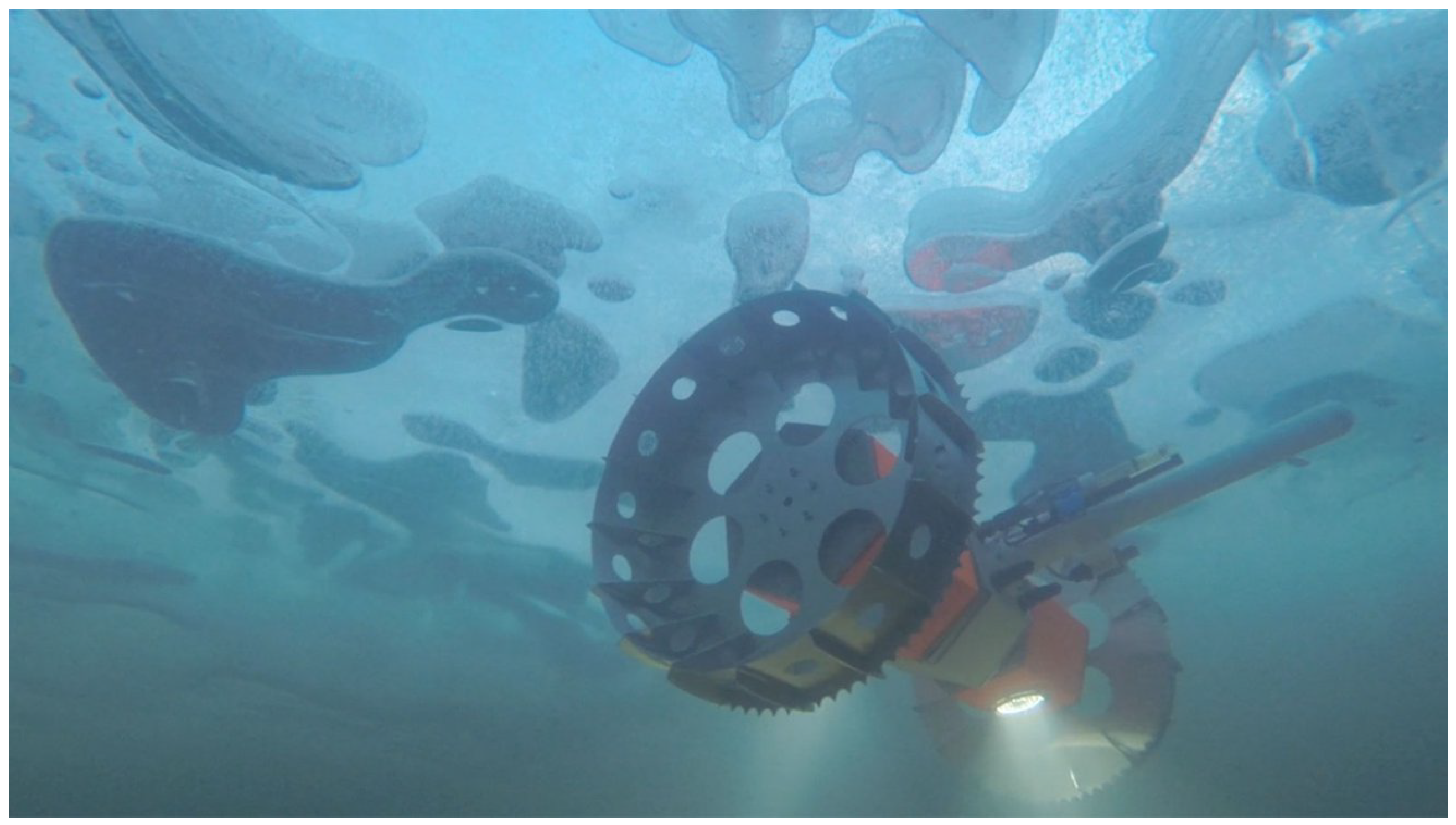
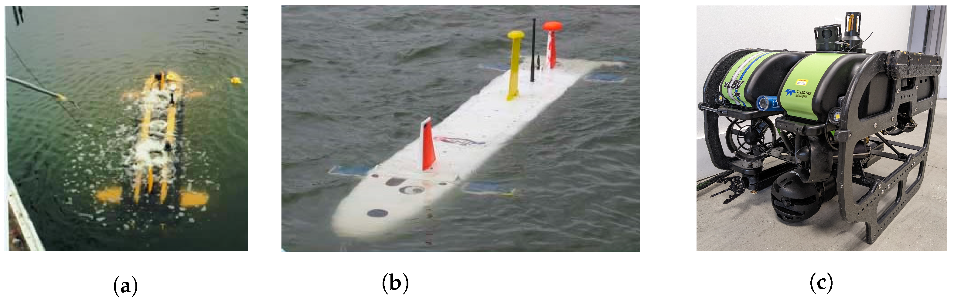

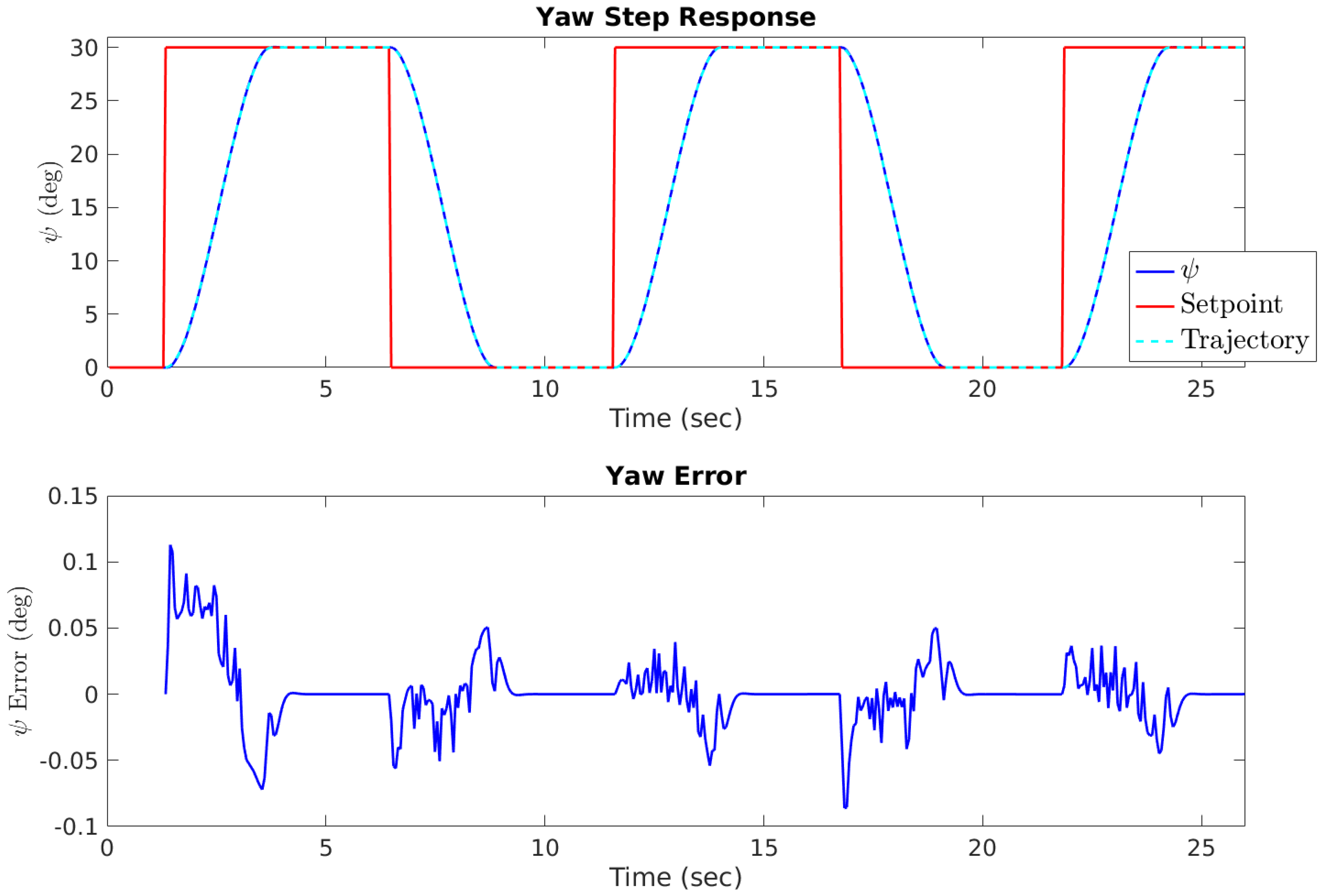

| Variable | Description |
|---|---|
| u, v, w, p, q, r | Body frame x, y, z, roll, pitch, and yaw velocities |
| , , | Inertial frame roll, pitch and yaw |
| Yaw control input | |
| Coefficient relating to yaw torque | |
| , , , , , | Added mass coefficients |
| , | Linear and nonlinear damping coefficient |
| , , | Moments of inertia |
| , , | Coordinates of the center of mass |
| , , | Coordinates of the center of buoyancy |
| m | Vehicle mass |
| g | Acceleration of gravity |
| V | Vehicle volume |
| Water density |
| Rise Time (s) | Settling Time (s) | Overshoot (deg) | Error (RMS deg) | |
|---|---|---|---|---|
| First Step | 2.362 | 2.608 | 0.104 | 0.0426 |
| Third Step | 2.413 | 2.425 | 0.083 | 0.0164 |
Publisher’s Note: MDPI stays neutral with regard to jurisdictional claims in published maps and institutional affiliations. |
© 2022 by the authors. Licensee MDPI, Basel, Switzerland. This article is an open access article distributed under the terms and conditions of the Creative Commons Attribution (CC BY) license (https://creativecommons.org/licenses/by/4.0/).
Share and Cite
Osler, S.; Sands, T. Controlling Remotely Operated Vehicles with Deterministic Artificial Intelligence. Appl. Sci. 2022, 12, 2810. https://doi.org/10.3390/app12062810
Osler S, Sands T. Controlling Remotely Operated Vehicles with Deterministic Artificial Intelligence. Applied Sciences. 2022; 12(6):2810. https://doi.org/10.3390/app12062810
Chicago/Turabian StyleOsler, Shay, and Timothy Sands. 2022. "Controlling Remotely Operated Vehicles with Deterministic Artificial Intelligence" Applied Sciences 12, no. 6: 2810. https://doi.org/10.3390/app12062810
APA StyleOsler, S., & Sands, T. (2022). Controlling Remotely Operated Vehicles with Deterministic Artificial Intelligence. Applied Sciences, 12(6), 2810. https://doi.org/10.3390/app12062810