Article

Model-Validation and Implementation of a Path-Following Algorithm in an Autonomous Underwater Vehicle †

1
Mechatronics Research Group (MRG), Tampere University (TAU), 33720 Tampere, Finland
2
Computer Vision and Robotics Institute (VICOROB), Universitat de Girona (UdG), 17003 Girona, Spain
*
Author to whom correspondence should be addressed.
This manuscript is an extended version of the conference paper: Villa, J.; Vallicrosa, G.; Aaltonen, J.; Ridao, P.; Koskinen, K.T. Model-based Guidance, Navigation and Control architecture for an Autonomous Underwater Vehicle. In Proceedings of the Global Oceans 2020: Singapore–US Gulf Coast, Biloxi, MS, USA, 5–30 October 2020; pp. 1–6.
Appl. Sci. 2021, 11(24), 11891; https://doi.org/10.3390/app112411891
Submission received: 5 November 2021 / Revised: 3 December 2021 / Accepted: 9 December 2021 / Published: 14 December 2021
(This article belongs to the Special Issue Underwater Vehicles)

Abstract

:
This article studies the design, modeling, and implementation of a path-following algorithm as a guidance, navigation, and control (GNC) architecture for an autonomous underwater vehicle (AUV). First, a mathematical model is developed based on nonlinear equations of motion and parameter estimation techniques, including the model validation based on field test data. Then, the guidance system incorporates a line-of-sight (LOS) algorithm with a combination of position PID controllers. The GNC architecture includes a modular and multi-layer approach with an LOS-based, path-following algorithm in the AUV platform. Furthermore, the navigation used in the path-following algorithm is developed based on a predefined coverage area. Finally, this study addresses simulation and field test control scenarios to verify the developed GNC architecture.

1. Introduction

Underwater research has become more relevant in scientific research due to the substantial amount of unexplored and unknown offshore areas. Remotely operated vehicles (ROVs) and autonomous underwater vehicles (AUVs) are the most popular vehicles for underwater exploration. These vehicles provide a solution for the exploration and exploitation of marine environments, reducing their costs and making the missions easier. Nonetheless, underwater research includes expensive and logistically complex field tests, while adequately accurate mathematical models from those vehicles can make these activities more accessible.
AUV maneuverability and controllability need to be studied based on an accurate mathematical model. This model is essential for the development of suitable guidance, navigation, and control (GNC) algorithms, along with simulation study purposes. The study of the mathematical model can use the theoretical six degrees-of-freedom (DOFs) dynamic model [1]. However, determining the hydrodynamic coefficients of this mathematical model is a complex and laborious activity due to the nonlinear characteristic and the coupled terms present in the model. These hydrodynamic coefficients were estimated by captive model tests, such as the planar-motion-mechanism system tests [2] or rotating arm experiments [3]. Kepler et al. [4] presented a method to predict those hydrodynamic coefficients requiring only the AUV’s geometry profile. Parameter estimation [5], and system identification (SI) [6] procedures can help to evaluate the hydrodynamic model coefficients based on field test data; here, several studies include these procedures in the development of mathematical models for AUVs. Kim et al. [7] proposed the estimation of the hydrodynamic coefficients based on the sliding mode observer and extended Kalman filter (EKF) nonlinear observers. Additionally, Cardenas and de Barros [8] used an identification approach combining an analytical and semi-empirical estimation method with a parameter estimator based on the EKF. MATLAB-Simulink software includes tools for both parameter estimation [9] and SI [10], providing simplicity in obtaining the mathematical model of the vehicle. Villa et al. [11] presented the mathematical model of an unmanned surface vehicle (USV) developed based on the MATLAB-Simulink SI, and the USV mathematical model was developed based on the parameter estimation method in [12]. Nonetheless, there is also a possibility of using online estimation instead of the described offline methods. Hong et al. proposed an online SI of AUV dynamics via in-field experiments. Regarding ground mobile robots, Fnadi et al. [13] developed a nonlinear observer for online estimation in real-time to enhance a linear–quadratic regulator (LQR) controller. Additionally, computational fluid dynamics (CFD) can be applied to estimate the hydrodynamic coefficients of complex AUV shapes [14,15].
Regarding the guidance system of the autonomous vehicle, the line-of-sight (LOS) is generally the default method for path-following and maneuvering control [16]. LOS is a guidance method that calculates the necessary heading reference angle of the vehicle to ensure convergence with a chosen path. Fossen and Pettersen [17] presented the stability proof for a class of proportional LOS guidance laws used for marine craft path-following control with no presence of ocean currents. Similarly, Fossen et al. [18] presented a nonlinear adaptive path-following controller for estimation and compensation of the sideslip angle, motivated by an LOS guidance principle. Moe et al. [19] introduced a guidance and control system in a horizontal plane movement including unknown ocean currents. Other control techniques in AUVs can include a constrained self-tuning controller for the heading and diving motions [20], and a unified receding horizon optimization scheme for the integrated path-planning and tracking control [21]. Additionally, Liang et al. [22] addressed a three-dimensional (3D) path-following control for underactuated AUVs with parameter uncertainties and external disturbances.
Coverage path-planning (CPP) determines a path that moves through all points of a certain area or volume of interest while bypassing obstacles [23]. This procedure allows for several applications, such as mine-countermeasure missions, search and rescue missions, seabed explorations, or offshore inspections. Classical methods include the exact cellular decomposition that divides the free space into simple, non-overlapping regions called cells. These cells, without obstacles inside, provide easy coverage and allow for robot sweeping with simple motions. One of the most used methods in the research field is the Boustrophedon cellular decomposition [24]. Nonetheless, this is defined as an offline method, as it assumes previous knowledge of the area and the polygonal obstacles. Most CPP methods consider the modeling of the environment as a simple planar surface. However, the underwater scenario is inherently 3D and requires a different CPP to cover these surfaces. Vidal et al. [25] proposed a novel 3D exploration and coverage methodology for AUVs. Hert et al. [26] presented an online 3D coverage algorithm based on a planar two-dimensional (2D) terrain-covering algorithm. Additionally, Galceran and Carreras [27] presented an offline 3D CPP algorithm that is suitable for covering seafloor areas, including 3D structure, operating on a bathymetric map.
This study continues the work presented in [28] for the design, modeling, and implementation of a path-following algorithm as a GNC architecture for an AUV. The previous work implemented a path-following algorithm for a predefined path, whose waypoints were defined based on a wall-detection algorithm. However, the dynamic coefficients of the vehicle were not accurate, and the mathematical model needed an improvement, with the necessary model validation. Moreover, the control system included a fixed yaw angle of the AUV equal to the slope of the detected wall. This paper develops a four DOFs mathematical model for the AUV using offline parameter estimation procedures based on field test data. This paper also validates an LOS-based, path-following algorithm with the experimental results from two control scenarios (simulation and field test) using the Girona500 AUV platform. First, the model validation allows for the estimation of the hydrodynamic coefficients in the AUV mathematical model. Then, this study advances the path-following algorithm presented in [28] by adding an LOS-based guidance system, which provides the required course angle for the path-following algorithm, allowing for continuous path operation. However, the motion control system does not compensate for environmental forces due to waves and ocean currents that affect the AUV’s performance to simplify the vehicle implementation. The path-following scenario is enhanced with additional waypoints, and is tested in both a water tank and a sea environment. This manuscript does not include the wall-detection algorithm developed in the previous work. Nonetheless, the AUV can incorporate it due to the modular architecture of the system.
This article proposes a path-following algorithm based on a GNC architecture for an AUV. In Section II, the AUV modeling and simulation are introduced based on the parameter estimation method to determine the four DOFs mathematical model of the vehicle. Then, in Section III, the control design is developed using a LOS-based guidance system with a series of position PID controllers. Additionally, this section defines the path-following waypoints based on a predefined planar coverage area. Finally, Section IV describes the GNC architecture implementation as modular and multilayer, and two control scenarios in simulation and field tests validate the proposed path-following algorithm.

2. AUV Modeling and Simulation

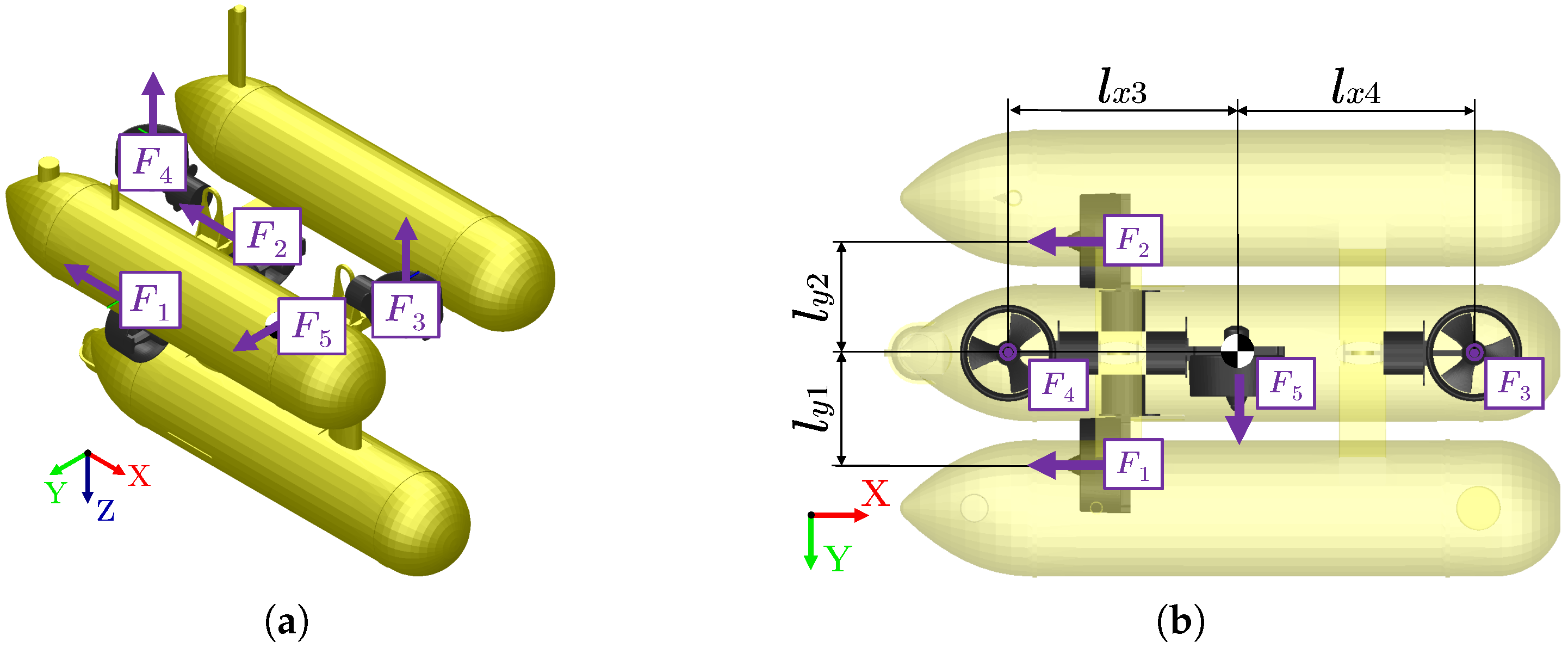
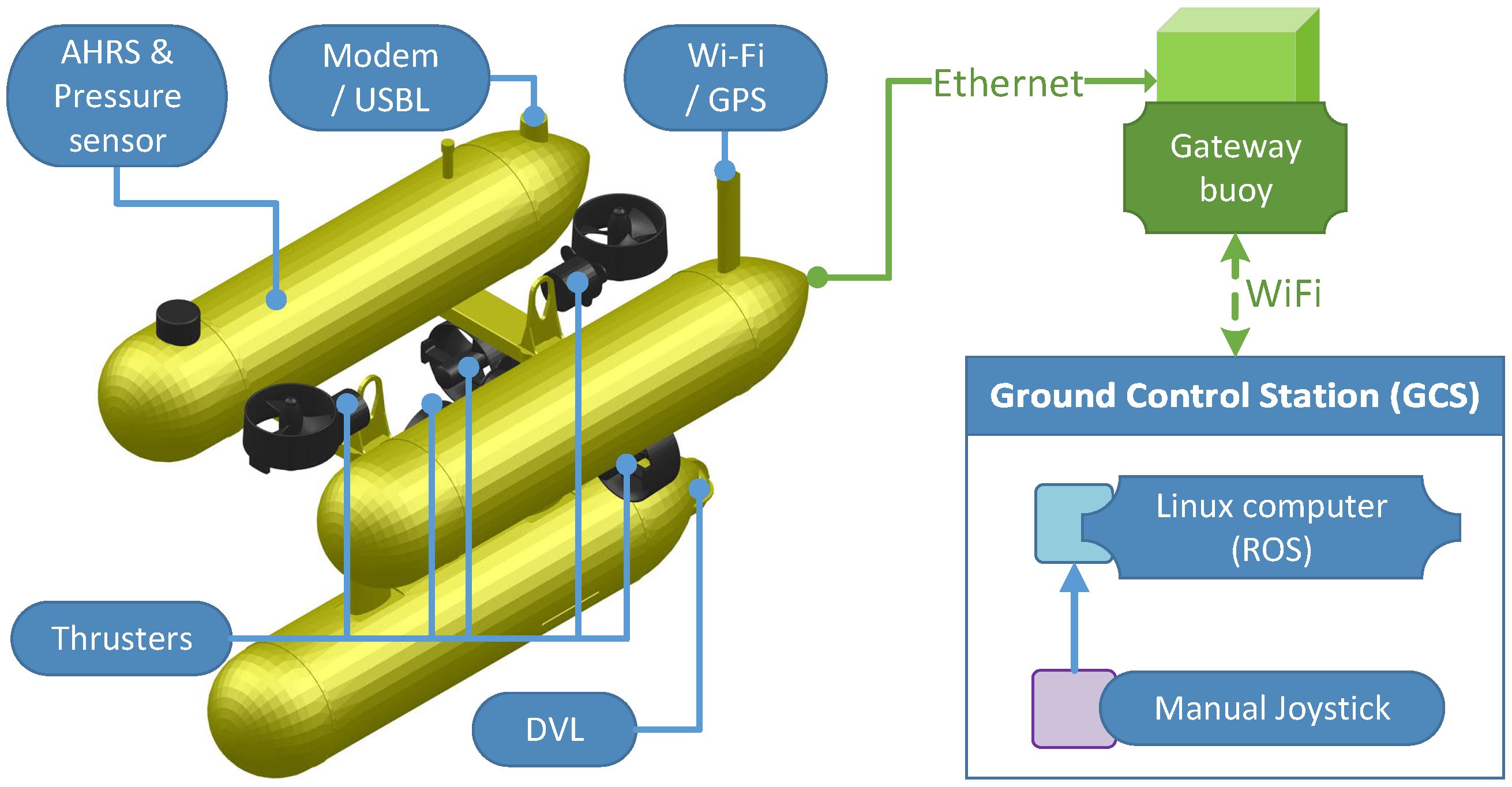
2.1. Overview of Girona500 AUV

This study utilizes the Girona500 AUV, a five-thruster configuration AUV that provides high configurability for various scientific instrumentation. This AUV has a multi-hull configuration, as it is composed of multiple streamlined hulls held together with a light frame. This approach incorporates the simplicity and stability of the open-frame platforms and also the low drag hydrodynamics of the torpedo-shaped vehicles [29]. Thus, the Girona500 AUV is perfectly suitable for survey and intervention capabilities.
The sensors and instrumentation included for the AUV navigation are mainly the attitude and heading reference system (AHRS), depth sensor, and doppler velocity log (DVL), as well as the GPS and ultra-short baseline (USBL). Figure 1 shows the block diagram with each navigation sensor connected with the localization filter, employing the Robot Operating System (ROS) framework [30]. This study uses the default navigation system from the COLA2 software architecture [31] and replaces its control system with the one developed during this article. The AUV navigator takes the data from the onboard sensors and merges them through a constant velocity model using an EKF. Furthermore, to initialize the vehicle position and bound dead-reckoning errors, the GPS receiver measures the vehicle position while, being at the surface, the pressure sensor calculates the vehicle’s depth, and the USBL system measures the vehicle position when submerged [32].
Figure 2 illustrates the simplified AUV model and includes its position and velocities. Moreover, the five-thruster configuration of the Girona500 AUV (see Figure 3) provides thrust forces in the surge, sway, heave maneuverings, or performing turns. The six DOFs AUV general motion uses the north–east–down (NED) local coordinate system. The following vectors η 6 DOFs and ν 6 DOFs consider the AUV positions and velocities in all six DOFs, respectively [16]
η 6 DOFs = N , E , D , ϕ , θ , ψ , ν 6 DOFs = u , v , w , p , q , r ,
where
  • N , E , D 
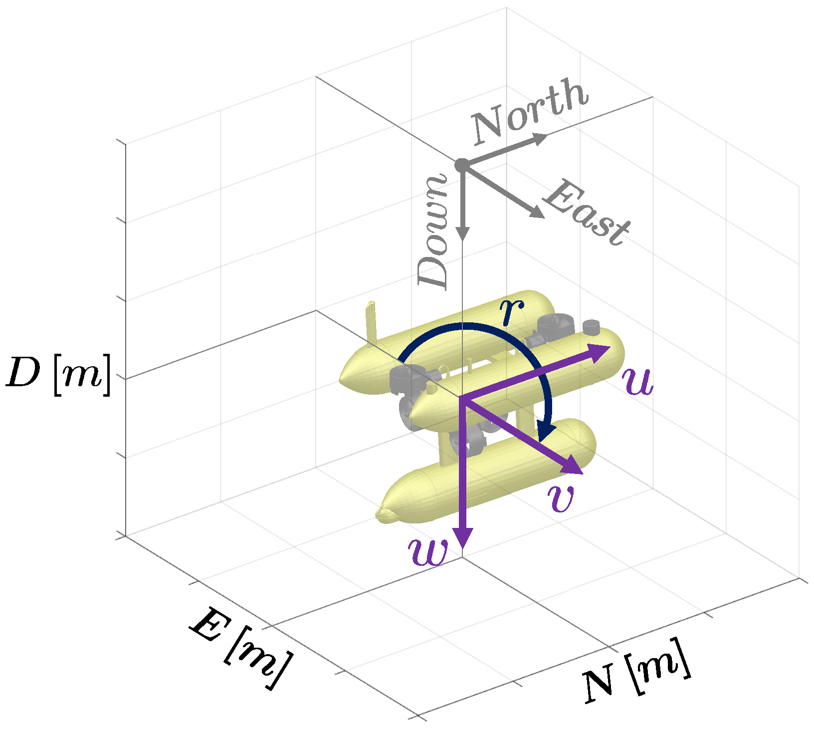
indicate to the NED positions in earth-fixed coordinates,
  • ϕ , θ , ψ define the Euler angles in earth-fixed coordinates,
  • u , v , w are the linear velocities based on the body-fixed reference frame,
  • p , q , r denote the angular velocities based on the body-fixed reference frame.

2.2. AUV Modeling

The AUV design and modeling have been analyzed based on the theoretical six DOFs dynamic model before the GNC algorithms’ implementation, whose dynamic model employs nonlinear equations of motion [1]. This study uses a reduced order for the four DOFs’ control, involving surge u, sway v, heave w, and yaw r, while neglecting the roll p and pitch q motions, as the AUV does not have actuation in all DOFs. Similarly to Equation (1), the reduced order for the four DOFs control uses the following AUV position η and velocity ν vectors:
η = N , E , D , ψ , ν = u , v , w , r ,
Thus, the dynamic model is simplified for the later parameter estimation of the dynamic coefficients of the AUV, and only the diagonal elements from the theoretical dynamic model are considered in this study. The hydrostatic forces and moments are related to buoyancy and weight, while the hydrodynamic forces and moments in an underwater vehicle refer to added mass and damping. This suggests that
M ν ˙ + C ( ν ) ν + D ( ν ) + g ( η ) = τ ,
where η and ν refers to the previously defined position and velocity vectors, g relates to the gravity and buoyancy body-fixed frame vertical forces, and M , D ( ν ) , C ( ν ) are the mass, damping, and Coriolis matrices, respectively. M and C ( ν ) involve added and rigid-body terms. The mass matrix M is determined as
M = M RB + M A = m X u ˙ 0 0 0 0 m Y v ˙ 0 0 0 0 m Z w ˙ 0 0 0 0 I z N r ˙ ,
where m is the mass of the vehicle, I z is the moment of inertia about the z-axis, and X u ˙ , Y v ˙ , Z w ˙ , and N r ˙ represent the hydrodynamic added mass coefficients.
The AUV actuators relate to the control forces and moments by
τ = T f ,
where T is the thrust configuration matrix of the AUV, and f is the control forces and moments vector. The five-thruster configuration matrix T considered in this study is defined by
T = [ 1.0 1.0 0.0 0.0 0.0 0.0 0.0 0.0 0.0 1.0 0.0 0.0 1.0 1.0 0.0 + l y 1 l y 2 0.0 0.0 0.0 ] ,
where l n = [ l x n , l y n , l z n ] denotes the distance from the AUV centre of mass to the thruster n. The considered AUV includes motions in surge and yawing (thrusters one and two), heave (thrusters three and four), and sway (thruster five). The thruster five is installed at the center of mass, not producing any rotational motion, as shown in Figure 3b.
C ( ν ) = C ( ν ) can perform the Coriolis-centripetal matrix C ( ν ) parametrization [33]. Nonetheless, the Coriolis and centripetal forces C RB ( ν ) and C A ( ν ) linearization about angular velocity equal to zero p = q = r = 0 suggests that the Coriolis and centripetal terms can be excluded from the dynamic mathematical model [34]. Moreover, the mathematical model is simplified, considering only surge, sway, heave, and yawing motions, so this study removes the Coriolis and centripetal terms at the four DOFs dynamic model.
The gravitational force acts through the center of gravity, while the buoyancy force acts through the center of buoyancy. In this case, the submerged weight of the body W and the buoyancy force B are given by
W = m g , B = ρ g ,
where ρ is the water density, g is the acceleration of gravity, and ∇ is the displaced volume of fluid by the vehicle. As pitch and roll angles are considered constant and equal to zero, the vector of gravitational and buoyancy forces and moments g is determined by
g = 0 , 0 , ( W B ) , 0 .
The damping terms involve both linear and quadratic damping [16]. However, it is usually challenging to differentiate these effects. The hydrodynamic damping matrix D ( ν r ) is the sum of the linear and the nonlinear terms, such that
D ( ν r ) = D lin + D nlin ( ν r ) ,
where D lin is the linear damping matrix produced by potential damping and possible skin friction, and D nlin ( ν r ) is the nonlinear damping matrix produced by higher-order and quadratic damping terms, defined by
D lin = X u 0 0 0 0 Y v 0 0 0 0 Z w 0 0 0 0 N r ,
D nlin ( ν r ) = X | u | u 0 0 0 0 Y | v | v 0 0 0 0 Z | w | w 0 0 0 0 N | r | r ν r .

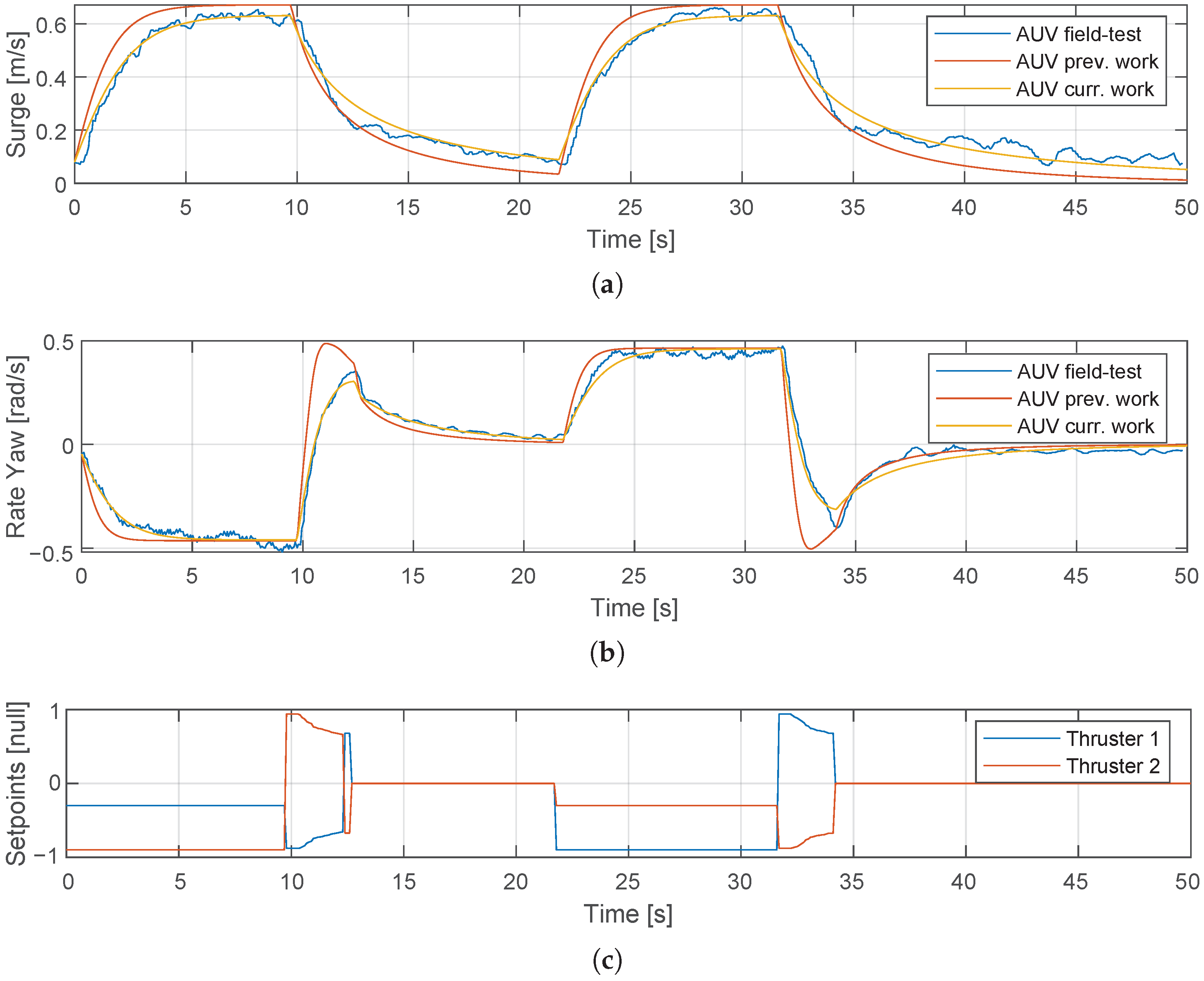
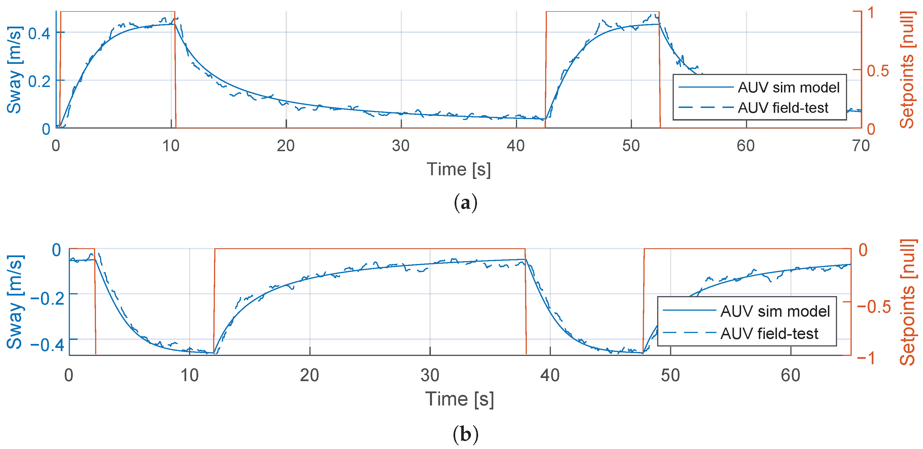
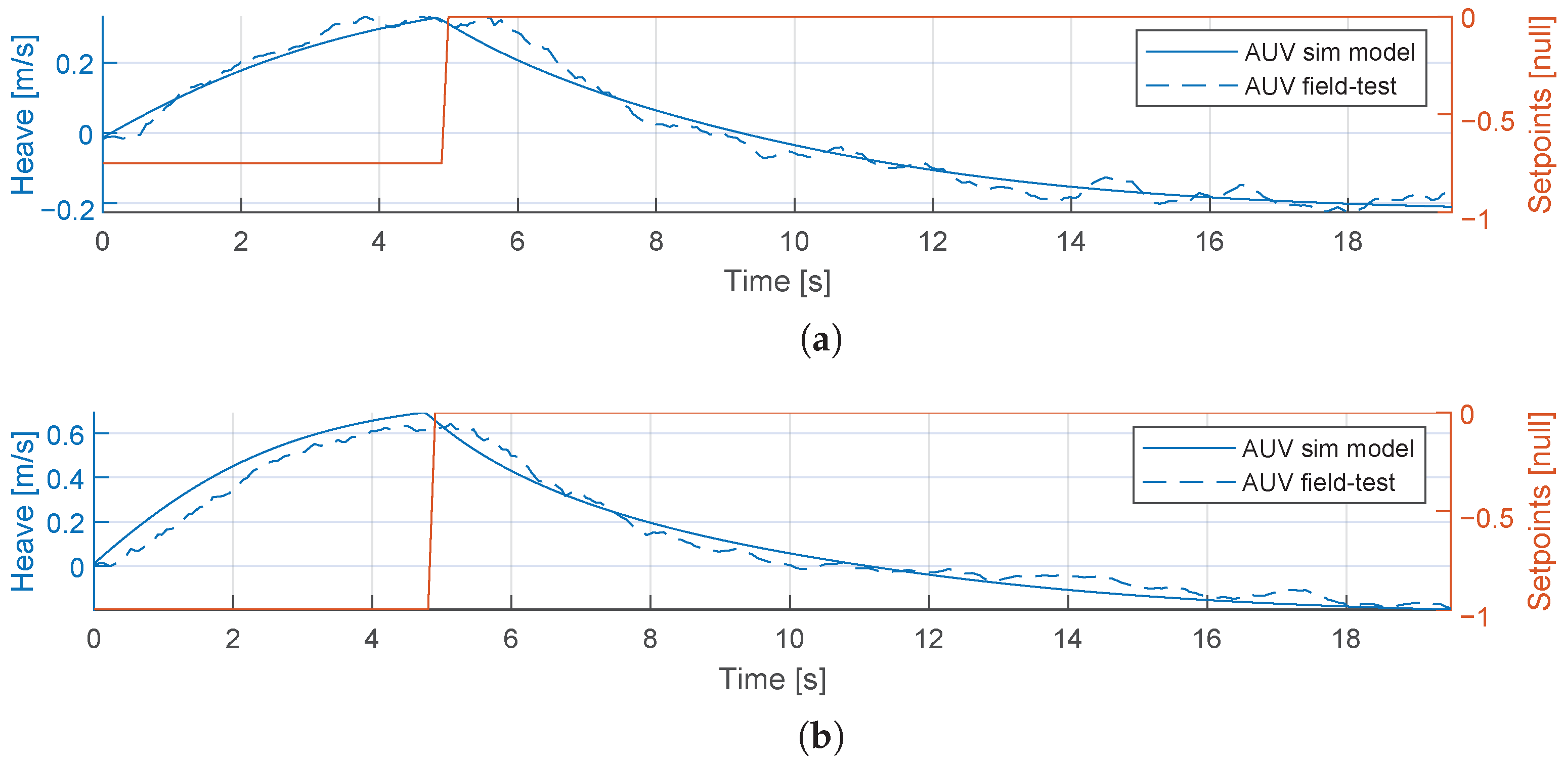
2.3. Model-Validation Using Parameter Estimation

The Girona500 AUV has an aluminum frame supporting three torpedo-shaped hulls, five thrusters, and all necessary scientific instrumentation. The strip theory [34,35] cannot be used to calculate the hydrodynamic coefficients of the AUV model, as the Girona500 AUV is not a torpedo-shaped hull with a cylindrical rigid body. Thus, this study requires a more advanced estimation method for this vehicle. Over-parametrization is the main problem when estimating parameters using SI or nonlinear optimization methods. The solution to this problem is to exploit theoretical information and estimate a model of partially known parameters [1].
The model validation includes four different parameter estimation runs. These test runs comprise independent surge, sway, heave, and yawing AUV motions, with different thruster setpoint values in all directions. These values comprise the 0.25, 0.50, 0.75, and 1.00, setting a constant input to the motion controllers. The test runs involve straight trajectories in the sway, and heave while having a zigzag pattern to estimate the hydrodynamic coefficients in the surge and yaw motions. This zigzag pattern is performed by setting constant control inputs to the thrusters for turning while moving forward with steady surge speed.
The estimation method uses the MATLAB-Simulink parameter estimation tool [9], employing a time-domain method for the AUV mathematical model. This estimation method minimizes the cost function using a nonlinear least-squares approach, evaluating the model until the estimation converges and terminates. With this parameter estimation tool, the running estimation will vary the selected model parameters—in our case, hydrodynamic coefficients—to reduce the error between the simulation outputs and the experimental data. The nonlinear least-squares method minimizes the squares of the residuals using the following minimization problem [9]
min x F ( x ) 2 2 = m i n x f 1 ( x ) 2 + f 2 ( x ) 2 + + f n s ( x ) 2 , s . t . x ̲ x x ¯
where f 1 ( x ) , f 1 ( x ) ,⋯, f 1 ( x ) represent the residuals, and n s is the number of samples.
Table 1 shows the constant values shared in the experiments since these are computed when constructing the vehicle. Table 2 presents the comparison between the hydrodynamic coefficients used in the previous work [28] and the results acquired from the parameter estimation tool. The previous work coefficients are obtained from the COLA2 simulation package [36]. The dynamic coefficients X u , X u ˙ , X | u | u relate to surge, Y v , Y v ˙ , Y | v | v to sway, Z w , Z w ˙ , Z | w | w to heave, and N r , N r ˙ , N | r | r to yaw motion.
Figure 4a,b compare the field tests and the four DOFs mathematical model results with the hydrodynamic coefficients used in the previous work [28] and the coefficients obtained from the parameter estimation in a zigzag pattern. Even though only diagonal coefficients are estimated by neglecting the dynamic matrices’ cross-terms, the mathematical model shows an accurate response compared to the field test data. Furthermore, the current parameter estimation improves on the previous work, as the maneuvering of the AUV mathematical model is closer to the field-test data in both surge and yaw motions. Figure 4c illustrates these control inputs as thruster setpoints commands, which are the inputs for the Girona500 AUV and are related to thrust forces by a polynomial function. Additionally, Figure 5 and Figure 6 shows the comparison of field test with the mathematical model for sway and heave motions, using two separate sets of data related to different thruster setpoints.

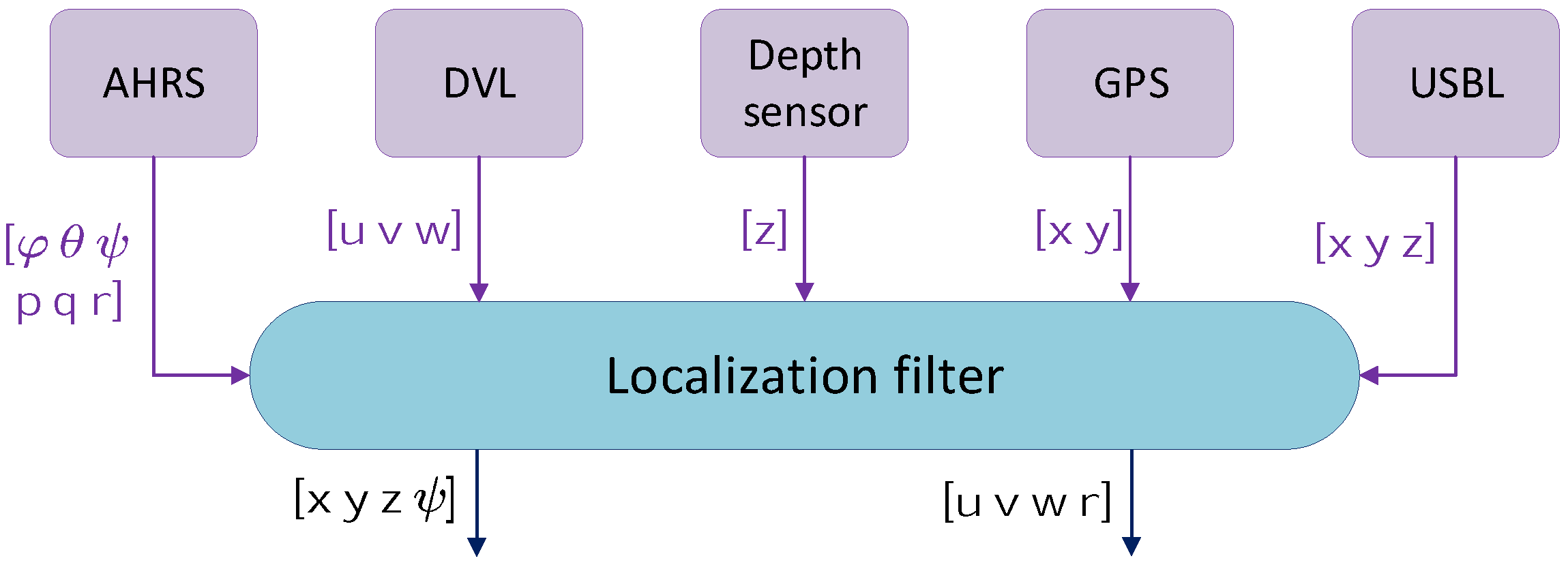
3. GNC System with LOS-Based Model

3.1. AUV Guidance System

The yawing motion control uses an LOS vector from the AUV position to the next waypoint, similar to [16]. This study focuses on a 2D covering algorithm, so the motion control system holds a constant depth for the heave motion in the LOS-based, path-following algorithm. The LOS-based guidance control determines the necessary course angle ψ d using the velocity-path relative angle χ r and the path-tangential angle χ p , where the lookahead-based steering is defined by
ψ d = χ p + χ r β ,
where the sideslip angle (drift) β is neglected to simplify the steering law [16]. The path-tangential angle χ p and the velocity-path relative angle χ r are defined as
χ p = atan2 ( E k + 1 E k , N k + 1 N k ) ,
χ r ( e ) = arctan ( K P e K I 0 t e ( τ ) d τ ) ,
where ( N k , E k ) and ( N k + 1 , E k + 1 ) are the positions of the reached and following waypoint, respectively, K P > 0 represents the proportional gain, and K I > 0 the integral gain. Finally, the cross-track error (normal to path) e ( t ) is defined as
e ( t ) = [ N AUV ( t ) N k ] sin ( χ p ) + [ E AUV ( t ) E k ] cos ( χ p ) .
The switching mechanism of the guidance system is defined as a combination of a sphere of acceptance [37] and reaches a predefined minimum yaw angle error. This cascade switching mechanism permits a continuous path operation to properly occur in all the waypoints at the path-following algorithm. The sphere of acceptance is defined as
[ N k + 1 N AUV ( t ) ] 2 + [ E k + 1 E AUV ( t ) ] 2 + [ D k + 1 D AUV ( t ) ] 2 R k + 1 2 .
where if the time AUV position ( N AUV ( t ) , E AUV ( t ) , D AUV ( t ) ) satisfies Equation (17), the course angle ψ d needs to be selected. Then, the next waypoint ( N k + 1 , E k + 1 , D k + 1 ) is chosen as a lookahead point whether the AUV’s yaw angle error is less than a predefined minimum angle.

3.2. AUV Control System

The motion control system of the AUV performs maneuvers in all translational motions (surge, sway, and heave) and in the yaw rotational motion with an individual PID controller for the north, east, and down positions and yaw orientation of the NED coordinate system. The separate PID controller approach is selected after comparing the velocity and position PID controllers in the previous study [28]. Furthermore, the motion control system does not involve compensation for the environmental forces due to waves and ocean currents that can affect the AUV’s ability to simplify the vehicle implementation. Table 3 shows the PID parameters used in this study. These parameters were estimated using the MATLAB-Simulink Control toolbox [38] for a certain time response ( T PID = 0.5 s) and transient behavior ( K tb = 0.9 ) parameter definition. Then, the AUV performed the necessary field tests in the sea environment to verify the correct PID parameters estimation in all motion controllers.

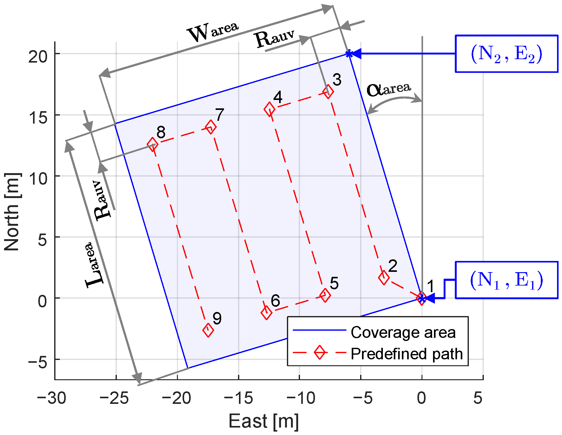
3.3. Coverage Path for the Path-Following Algorithm

The coverage path for the path-following algorithm in this study was obtained using a simple back-and-forth pattern in a predefined rectangular coverage area. The coverage area included no decomposition, while the path was parallel to the major axis, sweeping parallel to the North axis or parallel to the East axis to avoid unnecessary turns of the AUV. This approach fits in a search and rescue mission scenario, where the search area can be extensive without knowing the target’s position. The zigzag motion generation or seed spreader motions are thoroughly documented [24,39,40].
Figure 7 shows the implementation of the coverage path algorithm. The predefined rectangle coverage area is defined by the first two corners, origin ( N 1 , E 1 ) and second corner to be inspected ( N 2 , E 2 ), as well as the width W area of the coverage area. Additionally, the coverage radius R AUV of the AUV is predefined according to the perception sensor used in the vehicle. Based on the corners position and width, the algorithm calculates the length L area and rotation angle α area of the coverage area.
Figure 8 illustrates the AUV trajectory in the harbor of Sant Feliu de Guíxols, Girona, Spain, with the definition of each waypoint based on the coverage path algorithm. The coverage radius is limited to R AUV = 5 m, allowing more waypoints for the coverage path in the small field testing area. Meanwhile, the coverage area width is W area = 20 m, where the negative sign indicates that the AUV covers the left side of the vehicle.

3.4. Modular System for the Path-Following Algorithm

Figure 9 describes the modular GNC architecture with the required ROS topics. The coverage path module creates the waypoints for the path-following algorithm based on a predefined coverage planar area. Then, the guidance and control module receives the position and orientation of the AUV from the COLA2 navigation module [31]. The COLA2 navigation module includes the complete underwater localization of the Girona500 AUV. The LOS-based path-following algorithm is the only performance considered for analysis in the AUV implementation. The guidance and control module checks the AUV position to choose the next waypoint in the created trajectory and the necessary course angle for a continuous path operation. Furthermore, the guidance and control module incorporates the calculation of the required thruster setpoints based on the motion control system. The AUV thruster drivers receive these thruster setpoints to reach the defined waypoint from the coverage path.

4. Experimental Validation

4.1. System Implementation

The AUV incorporates multiple mechatronic systems to perform the path-following task and the motion control of the vehicle (surge, sway, heave, and yaw). Figure 10 presents the system overview of the AUV, which can be defined as high-level and low-level control. The high-level control involves the ROS computers with the GNC algorithms, and the low-level control involves the sensors and actuators of the AUV, which comprise an AHRS, depth sensor, DVL, thrusters, and the manual joystick controller.
The AUV runs most of the architecture inside the vehicle. The proposed GNC algorithms are included in an external Linux computer (ROS node) located onshore, connecting to the AUV by a gateway buoy via WiFi. Then, this buoy is connected to the AUV via ethernet. The implemented algorithms are obtained using the same procedure as the Standalone ROS-node [41], which provides a solution to the time-consuming process of C++ programming. The ROS master runs the previously described COLA2 navigation system and the developed GNC algorithms and sends the necessary thruster setpoints commands obtained from the motion control system.
The priority control level of this study is the same as presented in [28]. The highest priority in the control level is the manual joystick controller operated onshore, providing the necessary safety features by stopping the AUV movement at the user’s convenience.

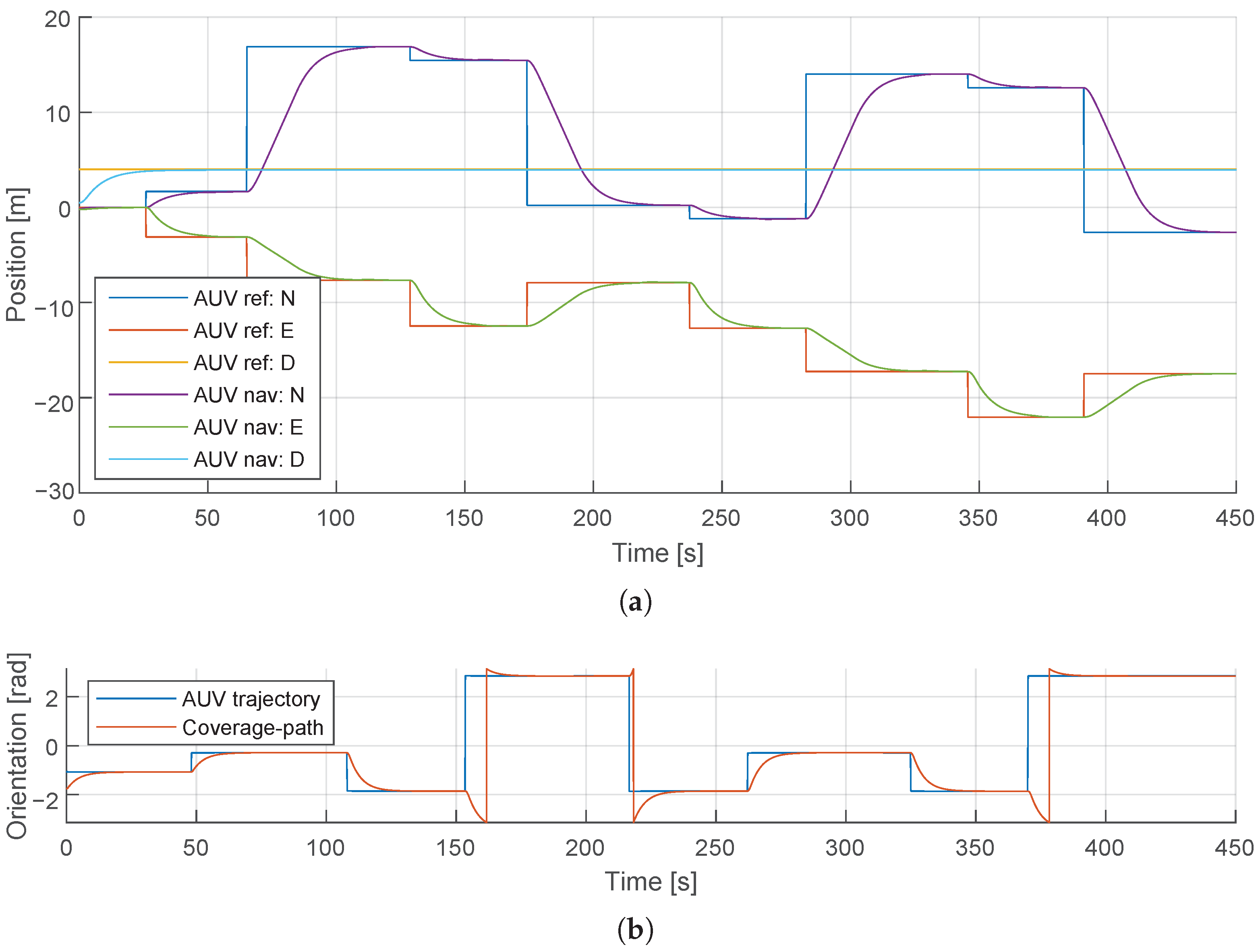
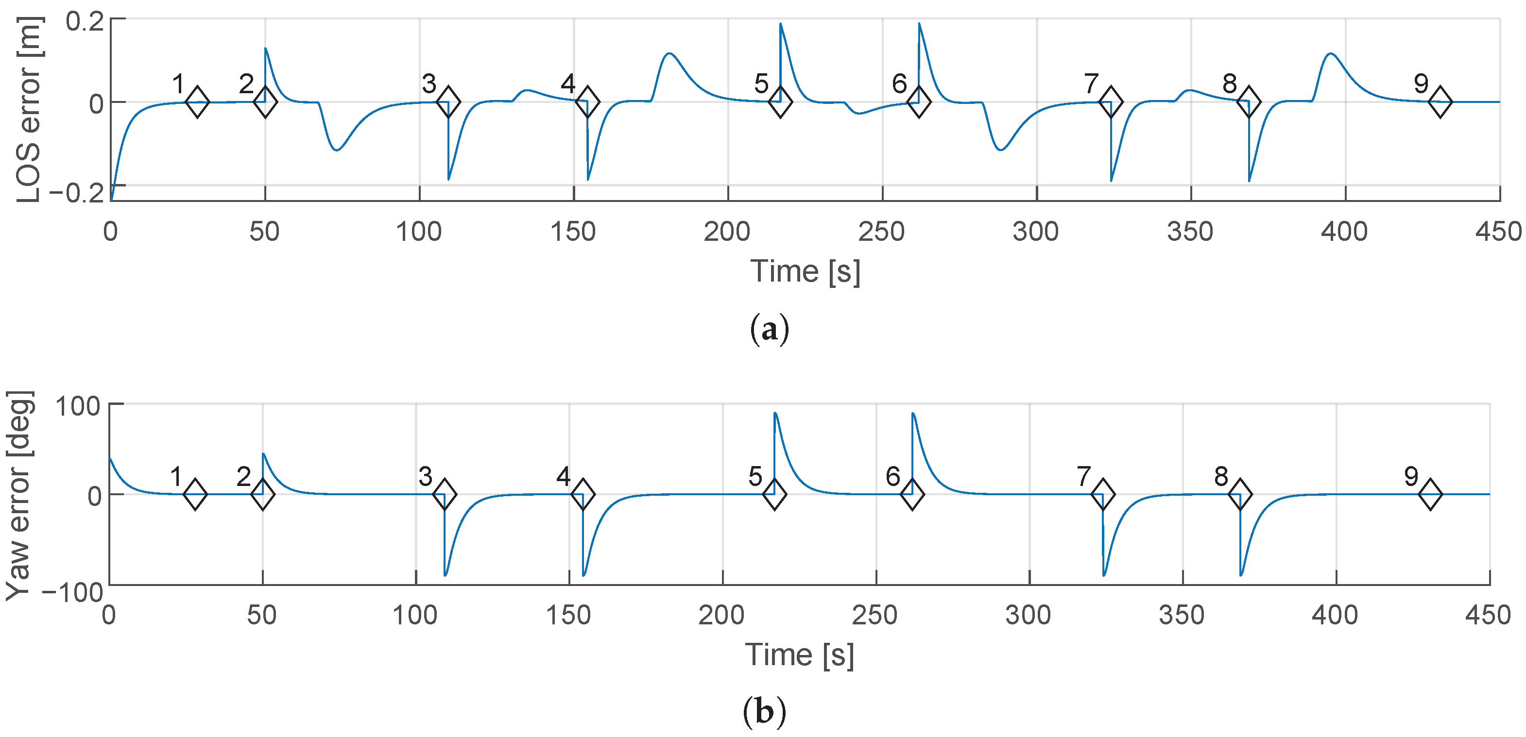
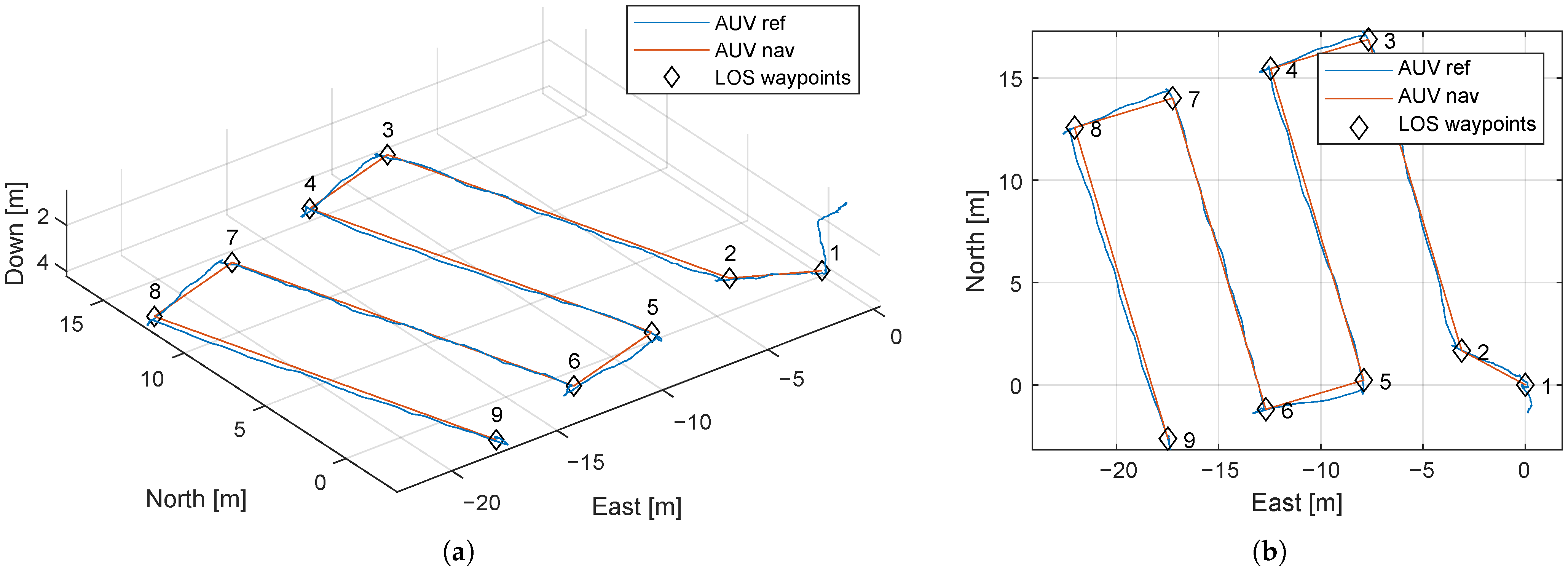
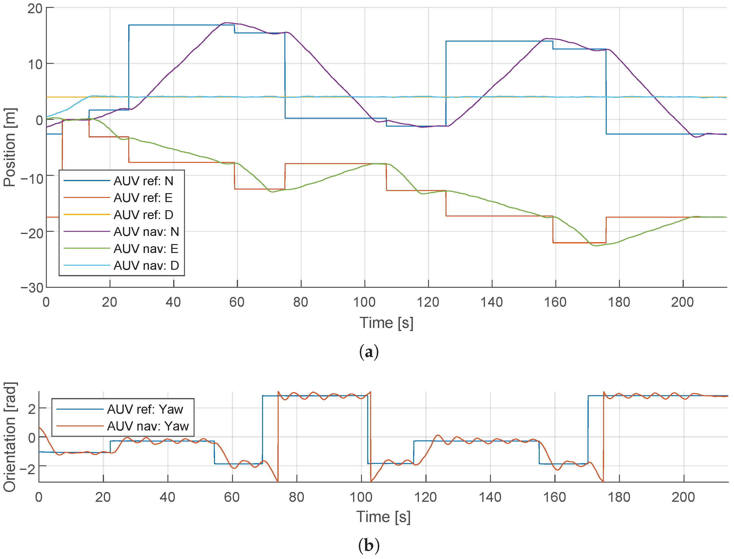
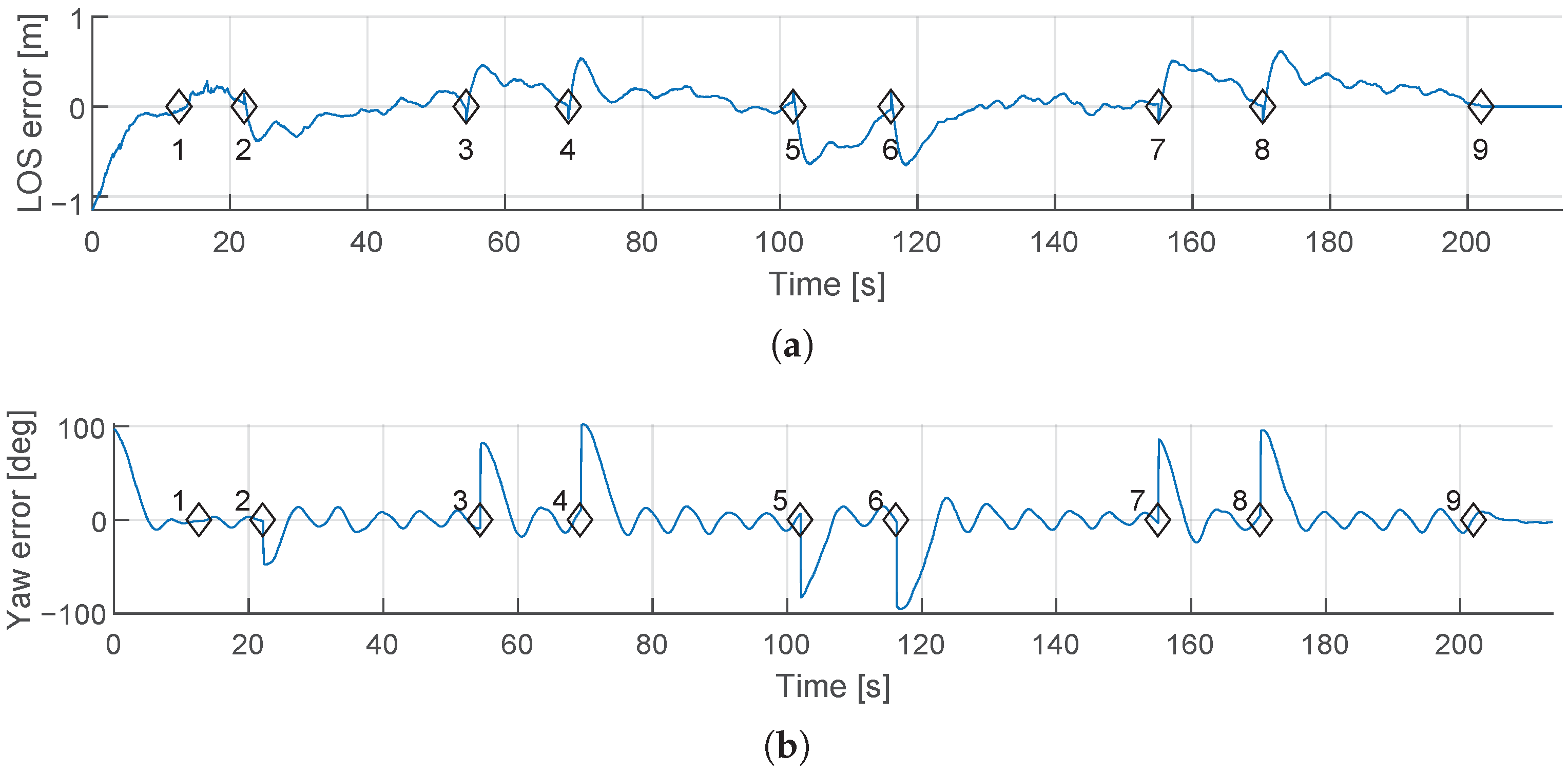
4.2. Simulation Results: Control Scenario I

The first control scenario simulates the AUV in an open environment and focuses on the path-following implementation, not including environmental disturbances in the system. From the coverage path algorithm, a series of waypoints in NED coordinates form the predefined path. Figure 11 illustrates the results for this simulation control scenario, including the north, east, and down positions and the yaw orientation. Moreover, Figure 12 illustrates the cross-track error e ( t ) and the yaw orientation error for the LOS-based, path-following algorithm in the simulation environment. These plots represent the previously discussed cascade switching mechanism, with the sphere of acceptance to show when the AUV has arrived at the desired waypoint and the requirement of less than 1 degree yaw angle error before moving to the next waypoint.
This scenario uses both the mathematical model developed of the AUV in Section 2 and the GNC architecture introduced in Section 3. The simulation tool for this control scenario uses the MATLAB-Simulink software, which can interactively simulate the AUV system model and show the results on scopes and graphical displays. The MATLAB-Simulink model includes the reduced-order AUV mathematical model to calculate the AUV position and velocities based on the total wrench generated from the PID controllers. The mathematical model uses the Equation (3), which contains the hydrodynamic coefficients from the parameter estimation approach shown in Table 2. Additionally, the AUV position and orientation act as navigation feedback for the LOS-based path-following algorithm, using a similar architecture to Figure 9.
This test validates the GNC algorithm using the LOS-based and position PID controllers approach, including the switching mechanism of the sphere of acceptance and reached angle. The AUV precisely generates the required trajectory for the LOS-based, path-following algorithm and reaches the final waypoint of the coverage path.

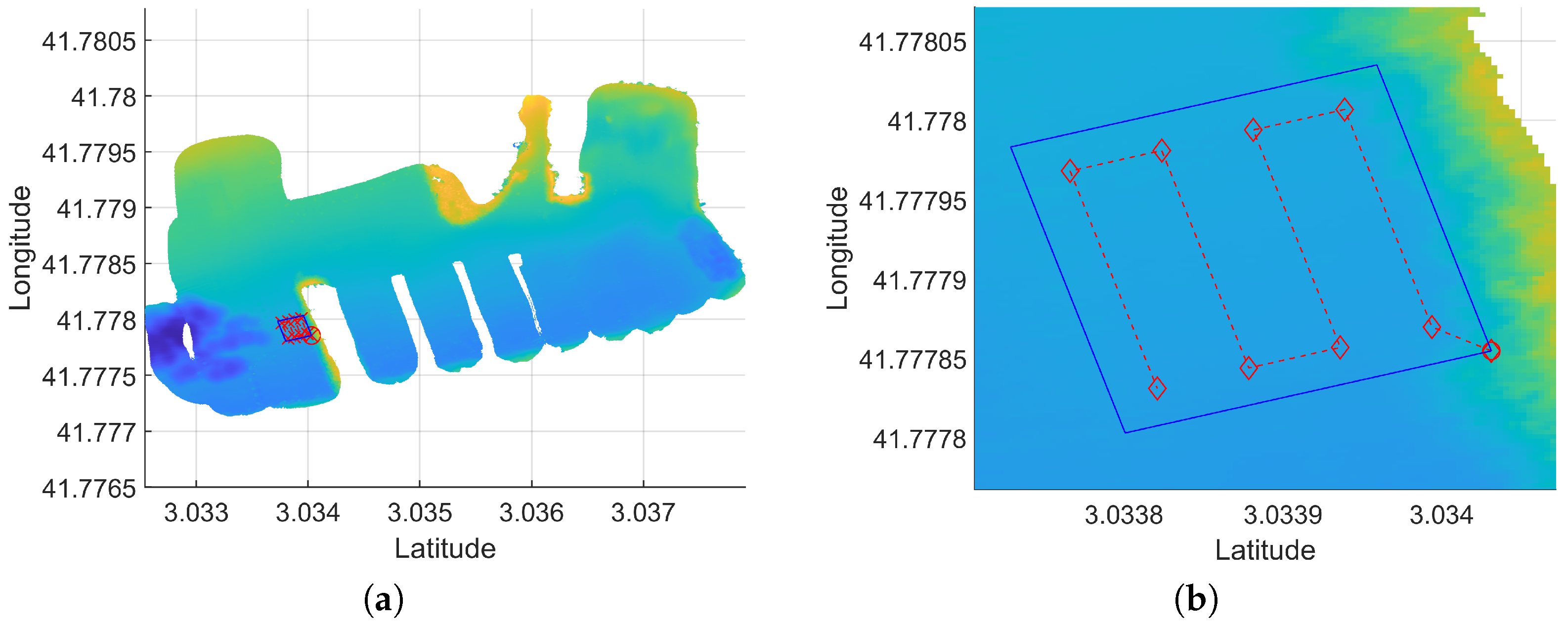
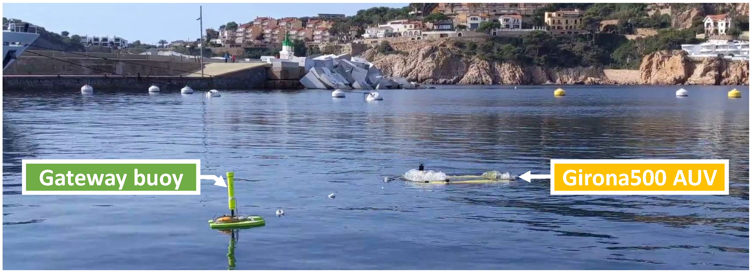
4.3. Experimental Results: Control Scenario II

The second test was implemented in the Girona500 AUV at the port of Sant Feliu de Guíxols (Girona, Spain), as shown in Figure 13. The implementation consists of a path-following of a predefined coverage planar area keeping a constant depth for the heave motion equal to 4 meters. The path-following experiments were performed successfully with the proposed GNC approach, as illustrated in Figure 14, where the red and blue solid lines are the coverage and actual AUV paths, respectively. In this control scenario, there was no current affecting the AUV, and the vehicle was located inside the harbor with good weather conditions and without the presence of significant waves during the field tests.
Figure 15 shows the input control values for the position PID controllers in the NED coordinate system. The implementation of the path-following algorithm performed correctly, reaching the ending waypoint of the coverage path. Nonetheless, there are differences between control scenario I and control scenario II, such as the total time of the test and behavior in the steady-state at yaw motion. These discrepancies are related to the reduced-order model and the non-inclusion of Coriolis and cross-terms of the dynamic matrices. Furthermore, the standalone ROS-node generated by MATLAB-Simulink can affect the results, as the simulation compiler differs slightly from the auto-generated C++ code.
Based on the cross-track error e ( t ) , three non-dimensional indicators measure the performance for the LOS-based, path-following algorithm: root–mean–square error (RMSE), mean absolute error (MAE), and standard deviation (SD). Table 4 includes these non-dimensional indicators showing the numeric values for control scenario II. Furthermore, Figure 16a illustrates the cross-track error e ( t ) for the LOS-based, path-following algorithm in the sea implementation. Even though the LOS-based, path-following performance is correct, there are oscillations in the yaw motion, as shown in Figure 16b, which need to decrease. As mentioned in Section 3, the PID controller parameters are estimated from the MATLAB-Simulink control toolbox, showing a great performance in the simulation environment; however, there is an oscillation in the yaw angle at steady-state for the implementation in the open environment at sea. A more accurate tuning of the PID parameters is required to reduce the oscillations in the yaw motion, including the integral parameter increase in the LOS PID controller to reduce the steady-state cross-track error. Both cross-track and yaw errors show the need for more advanced non-linear controllers required for applications in the underwater scenario. Nonetheless, these results show a correct, LOS-based, path-following performance, with the possibility of reducing the cross-track error with the future improvement in the control system by adding compensation to the environmental forces.

5. Conclusions and Future Work

This article focused on the four DOFs’ mathematical model development for an AUV using parameter estimation procedures based on field test data, along with the design and validation of an LOS-based, path-following algorithm in a simulation and an open environment at sea using the Girona500 AUV platform. The four DOFs mathematical model of the AUV was developed to verify the proposed GNC architecture. The model validation was based on parameter estimation procedures using field test data for surge, sway, heave, and yaw motions. After validating the AUV mathematical model, this paper developed the GNC system with an LOS-based, path-following algorithm with separate position PID controllers. This path-following algorithm used waypoints from a predefined coverage planar area. Finally, the experimental results showed two control scenarios in simulation and field tests, validating the designed GNC architecture and demonstrating its correct implementation.
Future work will include a comparison of this architecture with more advanced non-linear controllers and incorporate, comprehensive obstacle-avoidance abilities. These controllers will incorporate the environmental forces’ compensation to reduce the cross-track error of the LOS-based, path-following algorithm in the system.. Moreover, future work will improve the mathematical model of the AUV to study all six DOFs of the vehicle and all the cross-terms of the complete dynamic model.

Author Contributions

Conceptualization, J.V.; methodology, J.V.; software, J.V. and G.V.; validation, J.V. and G.V.; formal analysis, J.V.; investigation, J.V. and G.V.; resources, G.V.; data curation, J.V.; writing—original draft preparation, J.V.; writing—review and editing, G.V., J.A., P.R. and K.T.K.; visualization, J.V.; supervision, J.A. and K.T.K.; project administration, J.A., P.R. and K.T.K.; funding acquisition, P.R. and K.T.K. All authors have read and agreed to the published version of the manuscript.

Funding

This research was funded by the project MOCAV-G500 from EUMarineRobots that has received funding from the European Union’s Horizon 2020 (grant agreement No 731103), with the collaboration of the aColor project, which is funded by Technology Industries of Finland Centennial and Jane & Aatos Erkko Foundations. The APC was funded by the Faculty of Engineering and Natural Sciences (ENS) at Tampere University (TAU).

Conflicts of Interest

The authors declare no conflict of interest.

References

  1. Fossen, T.; Ross, A. Nonlinear modelling, identification and control of UUVs. IEE Control Eng. Ser. 2006, 69, 13. [Google Scholar]
  2. Gertler, M. The DTMB Planar-Motion-Mechanism System; David W. Taylor Naval Ship Research and Development Center: Washington, DC, USA, 1967. [Google Scholar]
  3. Comstock, J.P. Principles of Naval Architecture; Society of Naval Architects and Marine Engineers: Jersey City, NJ, USA, 1967. [Google Scholar]
  4. Kepler, M.E.; Pawar, S.; Stilwell, D.J.; Brizzolara, S.; Neu, W.L. Assessment of AUV Hydrodynamic Coefficients from Analytic and Semi-Empirical Methods. In Proceedings of the OCEANS 2018 MTS/IEEE Charleston, Charleston, SC, USA, 22–25 October 2018; pp. 1–9. [Google Scholar]
  5. Beck, J.V.; Arnold, K.J. Parameter Estimation in Engineering and Science; John Wiley & Sons: Hoboken, NJ, USA, 1977. [Google Scholar]
  6. Ljung, L. System identification. In Signal Analysis and Prediction; Birkhäuser: Boston, MA, USA, 1999; pp. 163–173. [Google Scholar]
  7. Kim, J.; Kim, K.; Choi, H.S.; Seong, W.; Lee, K.Y. Estimation of hydrodynamic coefficients for an AUV using nonlinear observers. IEEE J. Ocean. Eng. 2002, 27, 830–840. [Google Scholar]
  8. Cardenas, P.; de Barros, E.A. Estimation of AUV hydrodynamic coefficients using analytical and system identification approaches. IEEE J. Ocean. Eng. 2019, 45, 1157–1176. [Google Scholar] [CrossRef]
  9. The MathWorks, Inc. Simulink Design Optimization User’s Guide; The MathWorks, Inc.: Natick, MA, USA, 2009; Release 2020a. [Google Scholar]
  10. The MathWorks, Inc. System Identification Toolbox User’s Guide; The MathWorks, Inc.: Natick, MA, USA, 1988; Release 2020a. [Google Scholar]
  11. Villa, J.; Aaltonen, J.; Koskinen, K.T. Path-Following with LiDAR-based Obstacle Avoidance of an Unmanned Surface Vehicle in Harbor Conditions. IEEE/ASME Trans. Mechatron. 2020, 25, 1812–1820. [Google Scholar] [CrossRef]
  12. Villa, J.; Aaltonen, J.; Virta, S.; Koskinen, K.T. A Co-Operative Autonomous Offshore System for Target Detection Using Multi-Sensor Technology. Remote Sens. 2020, 12, 4106. [Google Scholar] [CrossRef]
  13. Fnadi, M.; Plumet, F.; Benamar, F. Nonlinear tire cornering stiffness observer for a double steering off-road mobile robot. In Proceedings of the 2019 International Conference on Robotics and Automation (ICRA), Montreal, QC, Canada, 20–24 May 2019; pp. 7529–7534. [Google Scholar]
  14. Tang, S.; Ura, T.; Nakatani, T.; Thornton, B.; Jiang, T. Estimation of the hydrodynamic coefficients of the complex-shaped autonomous underwater vehicle TUNA-SAND. J. Mar. Sci. Technol. 2009, 14, 373–386. [Google Scholar] [CrossRef]
  15. Pan, Y.; Zhang, H.; Zhou, Q. Numerical prediction of submarine hydrodynamic coefficients using CFD simulation. J. Hydrodyn. 2012, 24, 840–847. [Google Scholar] [CrossRef]
  16. Fossen, T.I. Handbook of Marine Craft Hydrodynamics and Motion Control; John Wiley & Sons: Hoboken, NJ, USA, 2011. [Google Scholar]
  17. Fossen, T.I.; Pettersen, K.Y. On uniform semiglobal exponential stability (USGES) of proportional line-of-sight guidance laws. Automatica 2014, 50, 2912–2917. [Google Scholar] [CrossRef] [Green Version]
  18. Fossen, T.I.; Pettersen, K.Y.; Galeazzi, R. Line-of-sight path following for dubins paths with adaptive sideslip compensation of drift forces. IEEE Trans. Control Syst. Technol. 2014, 23, 820–827. [Google Scholar] [CrossRef] [Green Version]
  19. Moe, S.; Pettersen, K.Y.; Fossen, T.I.; Gravdahl, J.T. Line-of-sight curved path following for underactuated USVs and AUVs in the horizontal plane under the influence of ocean currents. In Proceedings of the 2016 24th Mediterranean Conference on Control and Automation (MED), Athens, Greece, 21–24 June 2016; pp. 38–45. [Google Scholar]
  20. Rout, R.; Subudhi, B. NARMAX self-tuning controller for line-of-sight-based waypoint tracking for an autonomous underwater vehicle. IEEE Trans. Control Syst. Technol. 2016, 25, 1529–1536. [Google Scholar] [CrossRef]
  21. Shen, C.; Shi, Y.; Buckham, B. Integrated path planning and tracking control of an AUV: A unified receding horizon optimization approach. IEEE/ASME Trans. Mechatron. 2016, 22, 1163–1173. [Google Scholar] [CrossRef]
  22. Liang, X.; Qu, X.; Wan, L.; Ma, Q. Three-dimensional path following of an underactuated AUV based on fuzzy backstepping sliding mode control. Int. J. Fuzzy Syst. 2018, 20, 640–649. [Google Scholar] [CrossRef]
  23. Galceran, E.; Carreras, M. A survey on coverage path planning for robotics. Robot. Auton. Syst. 2013, 61, 1258–1276. [Google Scholar] [CrossRef] [Green Version]
  24. Choset, H.; Pignon, P. Coverage path planning: The boustrophedon cellular decomposition. In Field and Service Robotics; Springer: London, UK, 1998; pp. 203–209. [Google Scholar]
  25. Vidal, E.; Palomeras, N.; Carreras, M. Online 3D underwater exploration and coverage. In Proceedings of the 2018 IEEE/OES Autonomous Underwater Vehicle Workshop (AUV), Porto, Portugal, 6–9 November 2018; pp. 1–5. [Google Scholar]
  26. Hert, S.; Tiwari, S.; Lumelsky, V. A terrain-covering algorithm for an AUV. In Underwater Robots; Springer: Boston, MA, USA, 1996; pp. 17–45. [Google Scholar]
  27. Galceran, E.; Campos, R.; Palomeras, N.; Ribas, D.; Carreras, M.; Ridao, P. Coverage path planning with real-time replanning and surface reconstruction for inspection of three-dimensional underwater structures using autonomous underwater vehicles. J. Field Robot. 2015, 32, 952–983. [Google Scholar] [CrossRef] [Green Version]
  28. Villa, J.; Vallicrosa, G.; Aaltonen, J.; Ridao, P.; Koskinen, K.T. Model-based Guidance, Navigation and Control architecture for an Autonomous Underwater Vehicle. In Proceedings of the Global Oceans 2020: Singapore–US Gulf Coast, Biloxi, MS, USA, 5–30 October 2020; pp. 1–6. [Google Scholar]
  29. Ribas, D.; Palomeras, N.; Ridao, P.; Carreras, M.; Mallios, A. Girona 500 auv: From survey to intervention. IEEE/ASME Trans. Mechatron. 2011, 17, 46–53. [Google Scholar] [CrossRef]
  30. Quigley, M.; Conley, K.; Gerkey, B.; Faust, J.; Foote, T.; Leibs, J.; Wheeler, R.; Ng, A.Y. ROS: An open-source Robot Operating System. In Proceedings of the ICRA Workshop on Open Source Software; Kobe, Japan, 2009; Volume 3, p. 5. Available online: http://robotics.stanford.edu/~ang/papers/icraoss09-ROS.pdf (accessed on 1 December 2021).
  31. Iqua Robotics. COLA2 Wiki. Available online: https://bitbucket.org/iquarobotics/cola2_wiki/src/master/README.md (accessed on 1 December 2021).
  32. Palomeras, N.; Carrera, A.; Hurtós, N.; Karras, G.C.; Bechlioulis, C.P.; Cashmore, M.; Magazzeni, D.; Long, D.; Fox, M.; Kyriakopoulos, K.J.; et al. Toward persistent autonomous intervention in a subsea panel. Auton. Robot. 2016, 40, 1279–1306. [Google Scholar] [CrossRef]
  33. Sagatun, S.I.; Fossen, T.I. Lagrangian formulation of underwater vehicles’ dynamics. In Proceedings of the Conference Proceedings 1991 IEEE International Conference on Systems, Man, and Cybernetics, Charlottesville, VA, USA, 13–16 October 1991; pp. 1029–1034. [Google Scholar]
  34. Fossen, T.I. Guidance and Control of Ocean Vehicles. Doctor’s Thesis, University of Trondheim, Trondheim, Norway, 1999.
  35. Antonelli, G.; Antonelli, G. Underwater Robots; Springer International Publishing: Cham, Switzerland, 2014; Volume 3. [Google Scholar]
  36. Iqua Robotics. COLA2 Simulation. Available online: https://bitbucket.org/iquarobotics/cola2_wiki/src/master/cola2_sim.md (accessed on 1 December 2021).
  37. Healey, A.J.; Lienard, D. Multivariable sliding mode control for autonomous diving and steering of unmanned underwater vehicles. IEEE J. Ocean. Eng. 1993, 18, 327–339. [Google Scholar] [CrossRef] [Green Version]
  38. The MathWorks, Inc. Simulink Control Design User’s Guide; The MathWorks, Inc.: Natick, MA, USA, 2004; Release 2020a. [Google Scholar]
  39. Lumelsky, V.J.; Mukhopadhyay, S.; Sun, K. Dynamic path planning in sensor-based terrain acquisition. IEEE Trans. Robot. Autom. 1990, 6, 462–472. [Google Scholar] [CrossRef]
  40. Acar, E.U.; Choset, H.; Rizzi, A.A.; Atkar, P.N.; Hull, D. Morse decompositions for coverage tasks. Int. J. Robot. Res. 2002, 21, 331–344. [Google Scholar] [CrossRef]
  41. The MathWorks, Inc. ROS Toolbox User’s Guide; The MathWorks, Inc.: Natick, MA, USA, 2019; Release 2020a. [Google Scholar]
Figure 1. Implemented filter in the localization and mapping system for the Girona500 AUV.
Applsci 11 11891 g001
Figure 2. Simplified AUV model utilizing the NED local coordinate system. AUV motion is represented by surge u, sway v, heave w, and angular velocity r around the z-axis.
Applsci 11 11891 g002
Figure 3. Considered AUV with its five-thruster configuration: (a) Thrust forces directions, (b) Distances from AUV center of mass to thrusters.
Applsci 11 11891 g003
Figure 4. Comparison of previous work and the parameter estimation in the current work for the Girona500 in forwarding zig-zag motion: (a) Surge, (b) Yaw motion, (c) Thruster setpoints.
Applsci 11 11891 g004
Figure 5. Model-validation using parameter estimation for the Girona500: (b) Sway (right side) motion (thruster setpoints equal to 1.00), (b) Sway (left side) motion (thruster setpoints equal to −1.00).
Applsci 11 11891 g005
Figure 6. Model-validation using parameter estimation for the Girona500: (a) Heave motion (thruster setpoints equal to −0.75), (b) Heave motion (thruster setpoints equal to −1.00).
Applsci 11 11891 g006
Figure 7. Coverage path definition based on Algorithm 1: Coverage path (dotted red line) is generated based on the dimensions l area , W area , and first two corners of the coverage area ( N i , E i ), along with the coverage AUV radius r AUV .
Applsci 11 11891 g007
Figure 8. Bathymetry map with the coverage area (blue line) and predefined path (dotted red line) for the AUV in the harbor of Sant Feliu de Guíxols (Girona, Spain): (a) Map view, (b) Zoom view.
Applsci 11 11891 g008
Figure 9. Modular GNC architecture schematic. The two GNC modules (guidance and control and coverage path modules) run independent ROS nodes.
Applsci 11 11891 g009
Figure 10. System overview for the Girona500 AUV with high- (ROS computer), and low-level (sensors and actuators) control.
Applsci 11 11891 g010
Figure 11. AUV tracking trajectory for the simulation model in NED coordinate system: (a) North, East, and Down, (b) Yaw.
Applsci 11 11891 g011
Figure 12. AUV errors at the LOS-based, path-following algorithm in Control scenario I, including the respective waypoints marked with their order number: (a) Cross-track error [m], (b) Yaw orientation error [deg].
Applsci 11 11891 g012
Figure 13. Girona500 AUV during the implementation of the path following algorithm at the harbor of Sant Feliu de Guíxols (Girona, Spain).
Applsci 11 11891 g013
Figure 14. AUV tracking trajectory for the sea trials in NED coordinate system: (a) 3D view, (b) 2D view.
Applsci 11 11891 g014
Figure 15. AUV tracking trajectory for the sea trials in NED coordinate system: (a) North, East, and Down, (b) Yaw.
Applsci 11 11891 g015
Figure 16. AUV errors at the LOS-based, path-following algorithm in Control scenario II, including the respective waypoints marked with their order number: (a) Cross-track error, (b) Yaw orientation error.
Applsci 11 11891 g016
Table 1. Principal characteristics of the AUV.
ParameterValue
m180.00 kg
0.1837 m 3
I z 40.70 kg m 2
l y 1 0.2432 m
l y 2 0.2432 m
Table 2. Comparison of the AUV dynamic coefficients between previous work and the parameter estimation used in the current work.
ParameterPrevious WorkCurrent Work
X u −40.0−21.750
X u ˙ −90.0−250.184
X | u | u −163.0−216.423
Y v −40.0−6.192
Y v ˙ −90.0−580.969
Y | v | v −600.0−485.538
Z w −40.0−92.657
Z w ˙ −90.0−471.215
Z | w | w −600.0−189.788
N r −10.0−15.560
N r ˙ 0.0−44.297
N | r | r −80.0−69.364
Table 3. PID controller parameters for the AUV.
Controller K P K I K D
North151.3660.01061081.310
East151.3660.01061081.310
Down151.3660.01061081.310
Yaw63.4250.0037271.85
LOS0.03330.00.0
Table 4. Comparison of non-dimensional indicators for the AUV tracking trajectory.
VehicleRMSEMAESD
Girona500 AUV0.23460.15250.2345
Publisher’s Note: MDPI stays neutral with regard to jurisdictional claims in published maps and institutional affiliations.

