A Computationally Efficient Musculoskeletal Model of the Lower Limb for the Control of Rehabilitation Robots: Assumptions and Validation

Abstract

We present and validate a computationally efficient lower limb musculoskeletal model for the control of a rehabilitation robot. It is a parametric model that allows the customization of joint kinematics, and it is able to operate in real time. Methods: Since the rehabilitation exercises corresponds to low-speed movements, a quasi-static model can be assumed, and then muscle force coefficients are position dependent. This enables their calculation in an offline stage. In addition, the concept of a single functional degree of freedom is used to minimize drastically the workspace of the stored coefficients. Finally, we have developed a force calculation process based on Lagrange multipliers that provides a closed-form solution; in this way, the problem of dynamic indeterminacy is solved without the need to use an iterative process. Results: The model has been validated by comparing muscle forces estimated by the model with the corresponding electromyography (EMG) values using squat exercise, in which the Spearman’s correlation coefficient is higher than 0.93. Its computational time is lower than 2.5 ms in a conventional computer using MATLAB. Conclusions: This procedure presents a good agreement with the experimental values of the forces, and it can be integrated into real time control systems.

1. Introduction

Lower limb musculoskeletal models (MSM) constitute a powerful simulation tool with numerous applications in the field of sports and rehabilitation. Despite the progress made in lower limb MSM, they still have some drawbacks which affect their validity [1] and their usefulness in clinical applications [2]. These drawbacks are related with three fundamental aspects: (i) have a precise and adjustable kinematic model for each patient; (ii) keep the model complexity as low as possible; and (iii) experimentally validate the model.

First, joint kinematics must be able to accommodate specific rehabilitation movements and inter-subject variability. In effect, the knee kinematics model defines the estimated relative motion between relevant anatomical points, affecting the muscles’ lever arms and the calculated forces, hence it is important to use models that can be adapted to different peoples and ranges of movement [3]. Leardini et al. conducted an exhaustive review of the different joint models used in MSM [4]. Simple knee models using the revolute pair do not adequately represent its kinematics [5]. In contrast, other complex models, such as those presented by [6], provide good movement estimates, but require anatomical information that can only be personalized using medical imaging techniques. However, the most widely used models represent the knee joint using a mobile axis of rotation, whose position and orientation are related to knee flexion angle. This relationship is obtained experimentally in in vitro studies, which limits its realism and customization capacity [7], mainly when applied to people with medical conditions [8,9].

For this reason, other alternatives that are more adaptable to different subjects or conditions of movement have been developed. One approach is based on three-dimensional parallel mechanisms that attempt to simulate the geometry of the ligaments [10]. Unfortunately, they have the disadvantages of (i) needing complex personalization based on anatomical data that requires medical imaging [4], and (ii) being sensitive to the mechanical properties of the ligaments [11]. A simpler approach was proposed in Farhat et al. [12], which simulates the instantaneous axis of rotation through a four-bar mechanism obtained through a functional calibration procedure.

Second, the models must offer an adequate representation of the contribution of muscle groups to joint movement, which is usually associated with considering a higher number of muscles. The majority of models used in practice apply schemes similar to those introduced by Delp et al. [13], and improved by Klein Horsman et al. [14] and Arnold et al. [15], with numerous groups of muscles. Generally, it is assumed that increasing the complexity of the model will improve its validity [16,17]. However, increasing the number of muscles requires more information about their anatomical and physiological characteristics to calibrate the model [18]. In addition, the resolution of the problem of the redundancy of muscular actions becomes more difficult, requiring complex optimization algorithms with a high computational cost [19,20]. For this reason, in many works, adjacent muscles are grouped, or only a single set of muscles is considered when solving the redundancy problem [21].

Finally, the validity of MSMs is perhaps the main limitation for their use in clinical applications. Currently, some practical rules for the verification and validation of MSMs have been established [22]. Other important clinimetric properties, such as the reliability of the estimates, have also been addressed [23]. However, most of the published works are limited to comparing estimates with other previous models or to indirect validations based on the coherence between the levels of EMG activity and the estimated forces [20,24]. The works with direct validation, i.e., the magnitudes estimated by the model are compared directly with experimental measurements, are scarce, and are often limited to in vitro validations [25]. The results of these studies are difficult to extrapolate to clinical applications. Hence the interest in in vivo validation based on joint contact forces, measured from instrumented knee prostheses [16,26] has recently been increased. Although it is not a complete validation—only the contact forces are measured, not the muscular ones—the instrumented prostheses are the source of experimental data in vivo with measurements closest to the reality of the internal reactions in the knee joint.

One of the most recent and interesting applications of MSM is their inclusion within the control algorithm of the robotic systems devoted to rehabilitation exercises. The knowledge of the muscular and ligamentous forces during movement allows (i) to increase the patient’s safety during the process; (ii) to monitor the rehabilitation process over time, thus quantifying its progress; and (iii) to establish a priori what force levels are to be achieved during the movement in specific muscles [27].

Within the mechanical systems that constitute the core of robotic rehabilitation systems, two main types can be distinguished: open kinematic chains, mainly exoskeletons [28,29,30], and closed kinematic chains, mainly parallel robots. One of the main differences between exoskeletons [31] and parallel robots for knee rehabilitation (RPRs) [32] is that the RPRs exert mechanical actions on the distal end of the limb. For this reason, it is necessary to ensure that the forces transmitted by the robot terminal element (mobile platform) to the patient’s foot give rise to the desired actions on the knee. As a result, developing a precise and adjustable MSM for the estimation of the relevant forces in the knee, such as muscle, tendon, ligament, and tibial contact forces, while performing the exercise with the robot is of paramount importance for the practical implementation of RPRs [21]. Additionally, if the model is to be integrated into the RPR control scheme, it must be simple enough to be able to operate in real-time. Finally, the MSM must be verified experimentally, since the safety and evolution of the patient’s recovery from injury will depend on it.

In this research, we propose a simplified MSM lower limb model for the control of an RPR [33]. It is based on a scalable parametric model [12], with some adaptations to reduce the computational cost and thus operate in real-time [11]. The model has been validated by using data from the “Third Grand Challenge Competition to Predict in Vivo Knee Loads” [26,34].

2. Materials and Methods

As mentioned before, the main objective of this work is to improve the computational efficiency of the dynamic model of the lower limb introduced in Nidal et al. [12], such that it can be used in real-time control algorithms of parallel robots used in rehabilitation exercises. In this section: (a) an overview of the dynamic model is presented, (b) assumptions to improve its computational efficiency are provided, (c) a real-time algorithm is provided, and finally (d) the procedure that was used in its verification is presented.

2.1. Dynamic Model

Here is a quick overview of this model is presented. The reader can refer to the original article [12] for more detailed information.

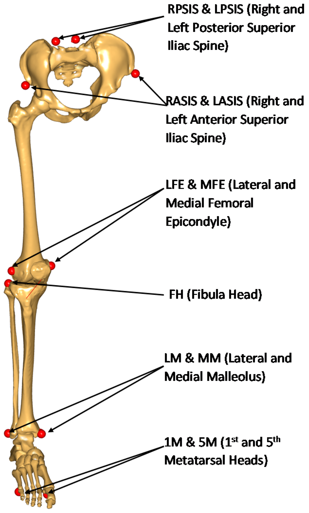
The lower limb is modeled by means of four segments: pelvis, femur, tibia, and foot. The joints are modeled as a three degrees-of-freedom (DOF) spherical joint at the hip joint center (HJC), a one-DOF four-bar mechanism at the knee, and a one-DOF revolute joint at the ankle joint center (AJC), leading to a total of five independent generalized coordinates. The inputs of the kinematic model are the coordinates of a set of anatomical landmarks, measured by a video-photogrammetry system (Figure 1).

The location of the HJC and the parameters of the four-bar mechanism that best match the actual motion of the knee are obtained in an offline stage using a functional calibration procedure [12]. For the location of the HJC, we use the method described in [35]. The four-bar mechanism that represents knee motion is determined using an optimal synthesis procedure based on the formulation of [36]. Furthermore, at this stage, (a) scaling is carried out to adjust the anatomical and joint characteristics as well as the inertial parameters of the model to the size of the subject, and (b) the local anatomical coordinate systems (ACSs) are defined. Later, in the online stage, the global positions of each parameter can be reconstructed from the motion of ACSs.

With respect to the dynamic model, the equation of motion was developed in the form of generalized forces using direct Jacobian transformation [12]:

$${\overrightarrow{\tau }}_I+{\overrightarrow{\tau }}_G+{\overrightarrow{\tau }}_{Mus}+{\overrightarrow{\tau }}_{Ext}=\overrightarrow{0}$$

(1)

where, ${\overrightarrow{\tau }}_{Mus}, {\overrightarrow{\tau }}_I,{\overrightarrow{\tau }}_G$, and ${\overrightarrow{\tau }}_{Ext}$ are the generalized forces corresponding to muscles, inertia, gravity, and external forces, respectively.

Note that the complete model includes all the inertial effects in ${\overrightarrow{\tau }}_I$. They were obtained basing on the inertial parameter calculated using the relations of Dumas et al. [37].

With respect to the muscles, they were modeled using via points and via cylinders approaches, as well as by considering the major muscles controlling the knee joint: eight flexors and ten extensors [14]. To solve the redundancy problem that exists in the calculation of muscle forces, minimizing the squared sum of muscle stresses was used as the optimization criterion. Once muscle forces were calculated, important knee forces such as the normal force on the meniscus and ligament forces were calculated from the free body diagram of the tibia.

2.2. Computational Efficiency Improvements

The following improvements were implemented to enhance the computational efficiency of the model:

• Since the model is applied to slow movements in rehabilitation exercises, the inertial forces are considered negligible compared to gravitational and external ones. Therefore, we assume a quasi-static model that does not depend on velocities and accelerations. As a result, the equation of motion expressed by Equation (1) can be represented by the following simple equation:

$${\overrightarrow{\tau }}_{Mus}=-\left({\overrightarrow{\tau }}_G+{\overrightarrow{\tau }}_{Ext}\right)$$

(2)

The generalized forces that correspond to weight and external forces, respectively, simply are:

$${\tau }_G=J_{G_{Fem}}^T{\overrightarrow{W}}_{Fem}^T+J_{G_{Tib}}^T{\overrightarrow{W}}_{Tib}^T+J_{G_{Foot}}^T{\overrightarrow{W}}_{Foot}^T$$

(3)

and:

$${\tau }_{Ext}=J_{P_{Ext}}^T{\overrightarrow{F}}_{Ext}+J_{{\omega }_{Foot}}^T{\overrightarrow{M}}_{Ext}$$

(4)

where $J_{G_{Fem}}^T,$ $J_{G_{Tib}}^T, J_{G_{Foot}}^T, J_{P_{Ext}}^T, \mathrm{and} J_{{\omega }_{Foot}}^T$ are the Jacobian matrices relating the generalized coordinates to the gravitational forces of the femur ${\overrightarrow{W}}_{Fem}$, tibia ${\overrightarrow{W}}_{Tib}$, the foot ${\overrightarrow{W}}_{Foot}$, the external force ${\overrightarrow{F}}_{Ext}$, and moment ${\overrightarrow{M}}_{Ext}$, respectively.

2.

We solve the redundancy problem by minimizing the squared sum of muscle stress. Therefore, the associated optimization procedure has a direct analytical solution by using Lagrange multipliers [2]. Thus, Equation (2) can be rewritten as follows:

$$-\left({\tau }_G+{\tau }_{Ext}\right)={\tau }_{Mus}=C_1{F}_1+C_2{F}_2+\cdots +C_n{F}_{n }$$

(5)

where, F_i represents the i-th muscle force, and C_i its coefficient or its contribution to the generalized force, which is calculated using the direct Jacobian transformation. The result of the optimization process is equivalent to Equation (6), extracted using Lagrange multipliers

$$F_i=\frac{A_i^2{C}_i{\tau }_{Mus}}{{{\displaystyle \sum }}_{j=1}^n{\left(A_j{C}_j\right)}^2}$$

(6)

where A_i represents the i-th muscle cross-sectional area as measured in [14]. It appeared here as a result of minimizing the squared sum of muscle stresses, as mentioned previously Hence, the optimization process can be omitted from the formulation of the dynamic model.

3.

The calculation of the muscle’s coefficients C_i—or moment arms—is a computationally high-cost procedure. This issue arises due to the number of muscles under consideration, their modeling, insertion points, and the corresponding Jacobian calculations. Fortunately, these coefficients are exclusively dependent on bone geometry and the current position. Therefore, they can be calculated in an offline process for all the possible combinations of the generalized coordinates in the dynamic system [2]. In this way, the muscle force calculation in the online stage is carried out directly using Equation (6) from the corresponding generalized muscle force value.

4.

The number of combinations associated with 5 DOF is too large. For example, for the squat exercise and assuming a discretization with a step of 1% of the range of each of the generalized coordinates, 3.2 × 10¹¹ possible combinations are obtained. However, this number can be drastically decreased by assuming a reduced number of functional degrees of freedom. Indeed, due to motor coordination, generalized variables do not change independently in repetitive movements. As a result, the number of independent parameters needed to describe this motion is lower than the total number of generalized coordinates. These independent parameters are called functional degrees of freedom (fDOF) [38]. This concept allows us to determine experimentally, and for each individual, the relationships between the main variable (the knee angle in our case) and the rest of the generalized coordinates of the model. Then, the combinations to be considered are reduced to the range of the main variable plus a narrow band of the rest of the variables around their average functions. These functions must be established in an offline process, carried out previously, in a kinematic calibration phase of the model.

After calculating the generalized muscle force τ_Mus using Equation (2), the muscle forces can be obtained directly by applying Equation (6). All of the previous equations are simple, direct, and computationally efficient, enabling the real-time calculation of muscle forces.

2.3. Real-Time Algorithm

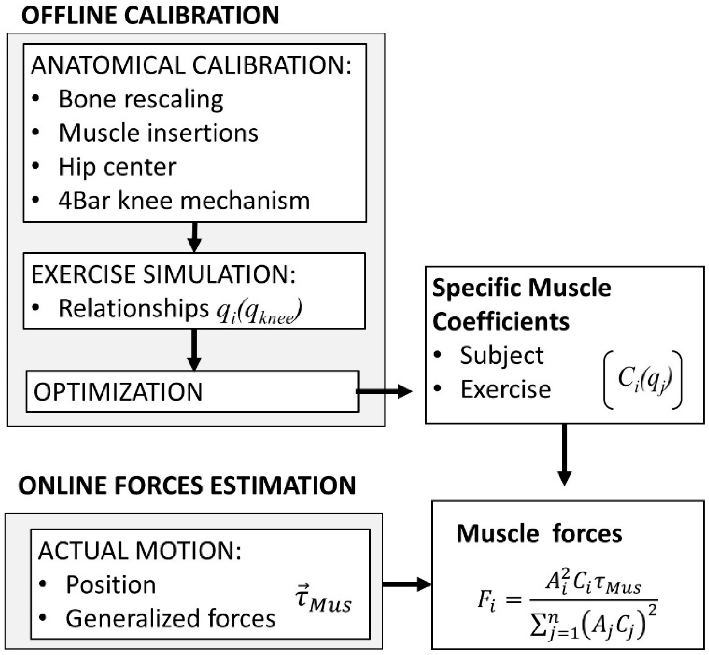
Figure 2 summarizes the two stages to apply the model: an offline calibration stage, and an online muscle and joint force calculation stage. The offline calibration stage consists of performing kinematic exercises for the anatomical, functional, and kinematic calibration of the model. The anatomical and functional calibration provides (1) the size of the modeled bone, (2) the parameters of the joints (HJC and four-bar mechanism), (3) the points of insertion of the muscles, and (4) the scale of the inertia parameters. This calibration is followed by a series of rehabilitation exercises to obtain the functional relationships between the kinematic variables. The workspace is discretized, and the coefficients of muscle force are calculated.

The model is then ready for online application in real time. The movement of the lower limb and its associated ACSs are reconstructed from the marker positions recorded by video photogrammetry. A force sensor measures the forces applied on the foot by the robot, while the gravitational forces are estimated from the masses and the positions of the centers of mass, which makes it possible to obtain the generalized muscle forces using Equation (2). According to the current value of the generalized coordinates, the values of muscle coefficients are retrieved from the stored offline values. Then, the magnitudes of muscle forces are calculated using Equation (6), as well as the internal reaction forces in the knee joint.

2.4. Verification and Validation

An experiment has been carried out to test the starting hypotheses and to verify the consistency of the model’s estimates with the levels of electromyographic activity. Furthermore, direct validation of the model’s estimates was carried out using in vivo experimental measurements based on data from Fregly et al. [26].

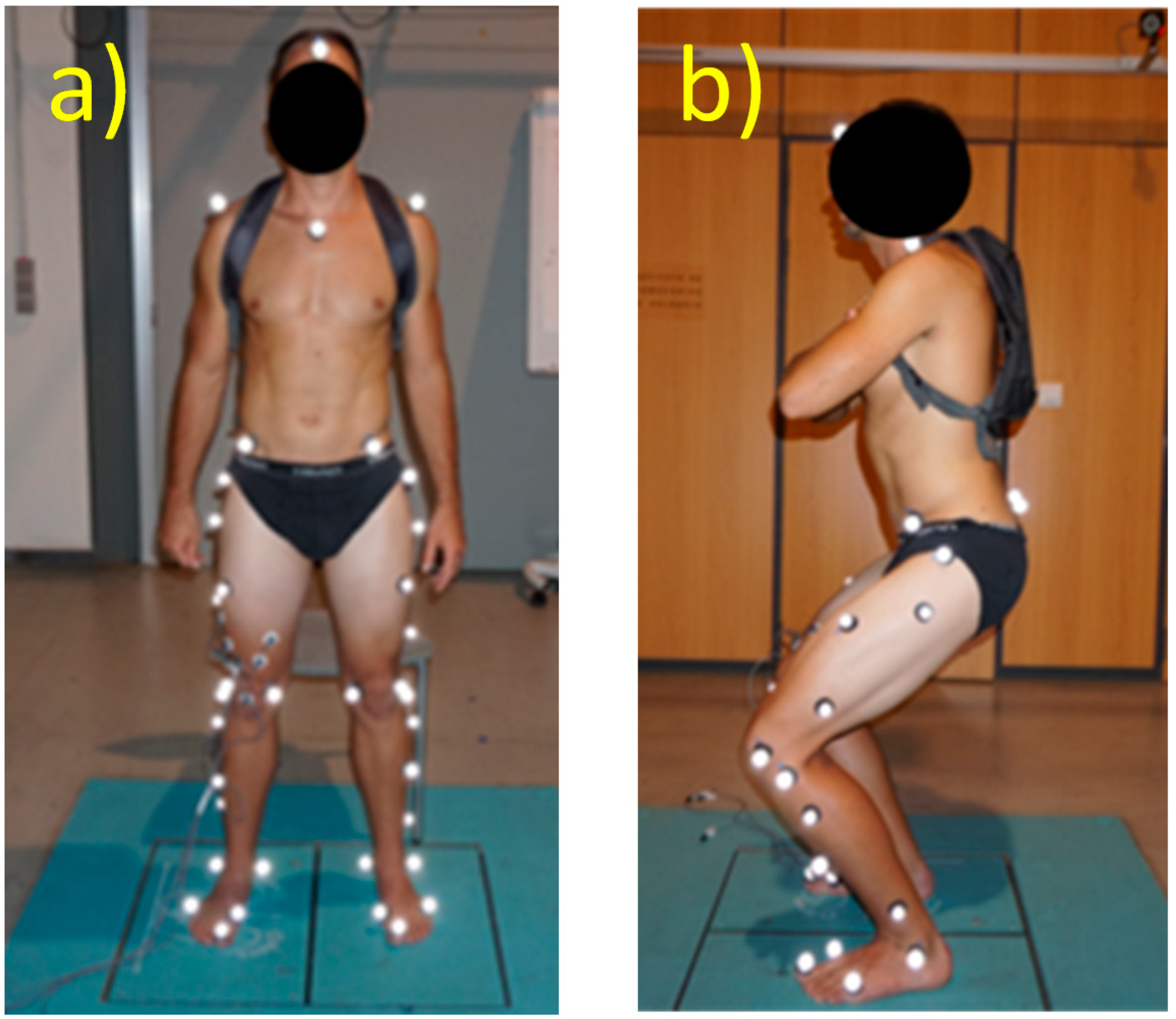
The verification of the model was performed using squat exercises (Figure 3). This motion imposes high force levels on the knee joint that induce higher moments and muscle forces than those resulting from normal gait motion. The experiment was approved by the Ethics Committee of the Universitat Politècnica de València, and all participants signed an informed consent document.

The subjects were asked to remain still in an upright, standing position, and a 5 s static trial was recorded. This trial was used for scaling the model. Subsequently, functional trials were performed enabling the functional calibration of the hip joint center, as well as the four-bar mechanism of the knee.

The considered squat exercise consisted of a repetitive cyclic motion, up and down with three load levels, in each of two trials: (i) with no load (L0), (ii) with a 6 kg backpack (L1), and (iii) with a 12 kg backpack (L2). Subjects were asked to perform approximately 5 slow repetitions of the squat, with their feet pointing forward, within 30 s.

Kinematic, dynamic, and EMG variables were recorded using conventional biomechanics instrumentation. External ground reaction forces were measured using a Dinascan/IBV force platform, and the movement was recorded using a Kinescan video–photogrammetry/IBV system [2]. Anatomical landmarks were used to scale the model and for the functional calibration [12]. The movements were recorded at 120 fps. Finally, EMG signals were measured with Noraxon Myotrace400 equipment (Scottsdale, AZ, USA). The equipment provides the RMS value (root mean square) of the EMG signal sampled at 1000 Hz. This signal was subsampled at 100 Hz, smoothed, and interpolated to obtain the values at the same time instants as Kinescan. The EMG electrodes were placed on the vastus medialis (VM) and vastus lateralis (VL), the biceps femoris, and the gastrocnemius according to the recommendations of SENIAM Project [39].

2.5. Data Processing and Statistical Analysis

The kinematic analysis was carried out from the coordinates of the markers, using the algorithms described in Page et al. [40]. For this study, two approaches were used to estimate the muscle forces: the full dynamic model (FDM) described in Farhat et al. [12], and the static geometric model (SGM) proposed here, using Equations (3)–(6).

Based on the experimental data, we have made the following verifications:

• Verification of the hypothesis of one functional degree of freedom. The degree of dependence of the generalized coordinates on the main variable (knee angle) has been calculated using a determination coefficient [41]. This coefficient was calculated for each of the different load conditions (0 kg, 6 kg, and 12 kg) for the five subjects. For these 45 measurements, the median and interquartile range were obtained.
• Verification of the hypothesis that inertial forces are negligible. We quantified the agreement between the generalized forces calculated from FDM and SGM. Concordance was assessed using the intraclass correlation coefficient (ICC) and the standard error of measurement (SEM). These calculations have been carried out in a functional way, obtaining a value for each trial (n = 15, 5 subjects × 3 trials) [42].
• Evaluation of the concordance between muscle forces as estimated using the SGM and the EMG measurements, using Spearman’s correlation coefficient (n = 75, five subjects, three trials, five cycles).
• Predictive ability of the model. Trials with load conditions L0 and L2 were used to establish a functional relationship between the muscle forces estimated by the model, VL and VM muscles using SGM, and the corresponding EMG signals observed (rms value). This functional relationship was used to estimate the forces in the same muscles for load condition L1 as a function of the corresponding EMG signals (rms) only. These new muscle estimates are referred to as FVLemg and FVMemg. For verification, they were compared with the same muscle values obtained by the model for the same load conditions. The comparison was made using ICC and standard error of the mean SEM, as described in point 2 (n = 25, five subjects, one trial, five cycles).
• Finally, a comparison was made between the internal reaction forces of the knee as estimated by our model and as measured experimentally in Fregly et al. [26]. We used ICC and SEM, as described in Points 2 and 4.

3. Results

The study involved five subjects, three females and two males (age 34.2 ± 10.3 years, mass 60.0 ± 6 kg, mean ± SD). For the validation of the model, we used the data of a woman from the “Third Grand Challenge Competition to predict in vivo knee loads” [26].

Each subject performed 5 continuous cycles for each of the three loading conditions (no load, L0; 6 kg load, L1; and 12 kg load, L2). Only measurements for the right leg were recorded.

Table 1. Kinematic characteristics of the movements (n = 15, five subjects x three load conditions).

Variable	Mean	STD
Knee ROM (°)	96.2	7.1
Max knee flexion angle (°)	106.5	5.9
Max flexion angular velocity (°/s)	81.2	25.0
Max extension angular velocity (°/s)	81.2	22.4

shows the kinematic characteristics of the movements (mean and SD) of the knee range (flexion–extension), and the corresponding maximum angular velocities in both directions. The mean range of flexion was 96.2°, with a maximum value of 106.5°. The mean maximum angular velocity was 81.2°/s in the flexion movement and somewhat faster (86.4°/s) in the extension movement.

Table 2. Summary of dynamic variables estimated using the full dynamic model FDM *. n = 15.

Variable	Mean Across Cycles. Mean (STD)	99 Percentile (All Cycles). Mean (STD)
Knee moment (N.m)	−29.5 (12.6)	11.1 (4.6)
VL force (N)	275.1 (117.9)	679.7 (222.8)
VM force (N)	117.8 (50.4)	290.6 (94.3)
Tibia normal force (N)	1018.0 (203.0)	1974.0 (364.0)
Tibia tangent force (N)	89.6 (30.7)	348.1 (71.6)

* The left column shows the mean and standard deviation of the mean values in each trial. The right column shows the mean and standard deviation of the maximum values, calculated as the 99th percentile for each trial. Knee moments are the moments associated with the gravitational, inertial, and external actions of the FDM. Positive knee moments are extensor, and negative moments are flexor.

describes the dynamic variables estimated by the full dynamic model (FDM). Knee moment had a negative mean value in the order of −30 Nm, with a maximum value of 11.1 Nm. It was negative during most of the movement, and needed to be balanced by the extensor muscles. As a result, the vastus lateralis muscle was active during most of the movement, exerting an average force of 275 N and a maximum value of 680 N. In the same way, the average and maximum forces induced by the vastus medialis were 118 N and 290 N, respectively. With respect to the reaction forces on the tibial plateau, the mean normal compressive force was 1000 N, and its maximum value was almost doubled, 1974 N. The forces in the tangential direction had much lower values (mean: 90 N; maximum: 350 N). The great dispersion of the forces obtained in the different tests should be noted. This may be due to differences between subjects and between load conditions.

The knee angle showed, on average, 99.2% of the variance of the other generalized coordinates (98.5% for the lowest quartile). This result confirms to the hypothesis that the movement has a single functional degree of freedom. Hence, it will be possible to estimate all generalized coordinates from the knee angle.

The correspondence between the FDM and SGM models is almost perfect (

Table 3. Agreement between FDM and SGM and Purely Geometric Model *. n = 15.

Model	ICC, Median (IQR)	SEM, Median (IQR)
SGM	1.000 (0.000)	0.042 (0.016)
Purely Geometric Model	0.999 (0.001)	0.957 (0.386)

* FDM: Full Dynamic Model. SGM: Static Geometric Model (the weights of the lower limbs are considered, but not the inertial forces). Purely Geometric Model: only the directly applied actions are considered, but not the gravitational or inertial forces. ICC: intraclass correlation coefficient. SEM: standard error of measurement, expressed as a percentage of the range of generalized force in the knee.

). The value of the ICC was 1.000 and the error resulting from neglecting the inertial forces is insignificant (less than 0.1% of the total range). The effect of the gravitational parameters on the estimation of forces is also limited, and hardly represents an average difference of the order of 1% of the range.

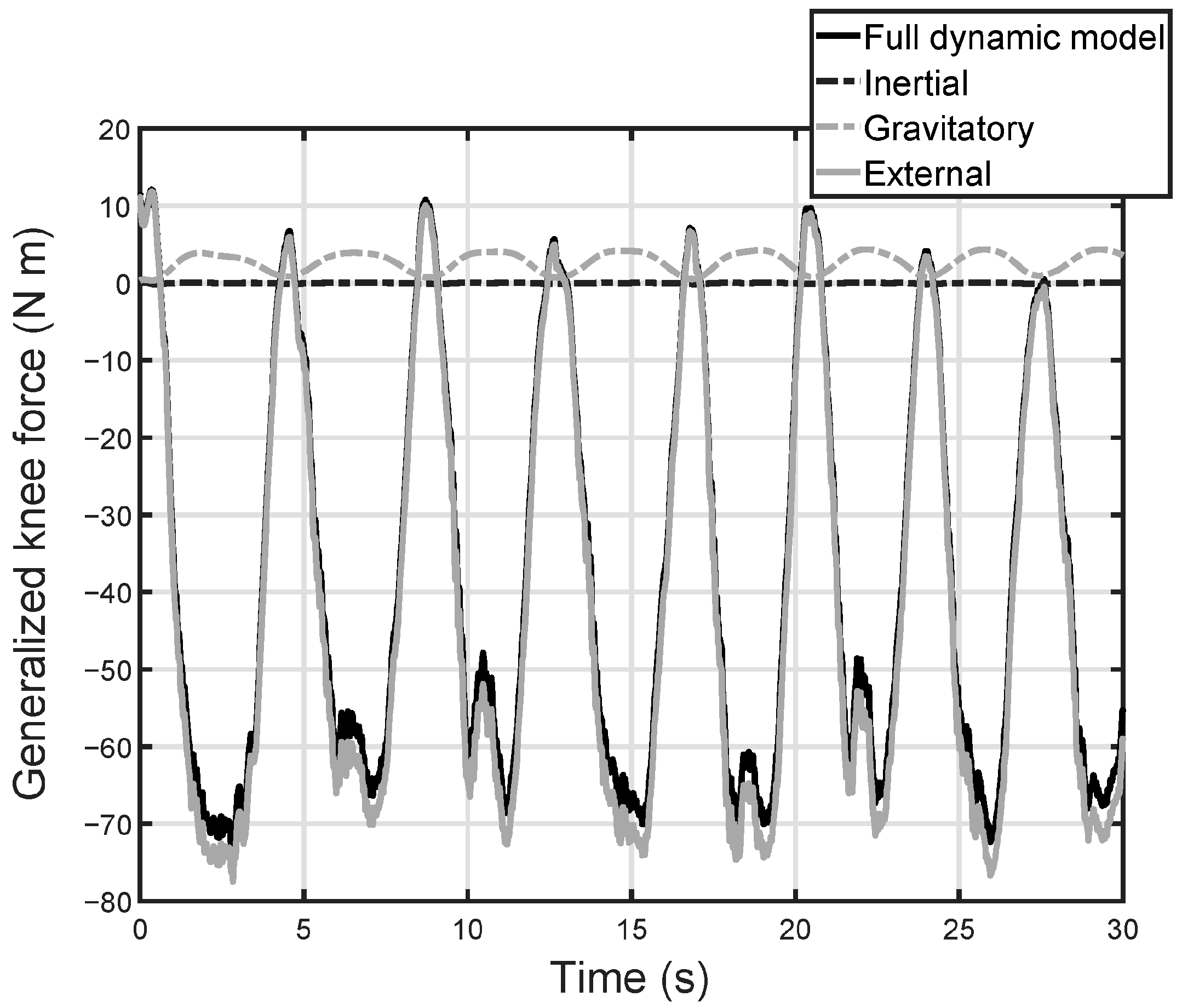
Figure 4 illustrates these results for a specific subject, showing the contributions of each component of the dynamic model to the generalized forces. As can be seen, the most important component is the external force on the foot. The force of gravity has a minor effect. The effect of the inertial components is negligible.

Table 4. Spearman’s correlation coefficients between measured EMG and muscle forces estimated by SGM. (n = 75).

MUSCLE	Extension. Mean (STD)	Flexion. Mean (STD)
Vastus lateralis	0.947 (0.038)	0.931 (0.068)
Vastus medialis	0.957 (0.032)	0.959 (0.019)

shows Spearman’s correlation coefficients between EMG signals as measured for the vastus medialis and vastus lateralis muscles, and the corresponding muscle force values as estimated by the SGM. Flexion and extension motions were separated for each cycle. We used 75 records for the flexion direction and the same number for the extension direction (five subjects, three trials, five cycles).

As can be observed, the correlation between the estimated muscle force and the measured EMG signals is excellent, with mean values higher than 0.93 for both muscles and both directions of motion. This reveals that model-based estimated muscle forces are coherent with the measured EMG values: they both increase and decrease in the same manner.

On the other hand,

Table 5. Agreement between the muscle force estimates by SGM and as estimated using Force–EMG calibration. The forces estimated by the SGM model for the L1 load condition are compared with the forces calculated from the Force–EMG calibration curves of the L0 and L2 conditions, using the EMG signal of the L1 tests. n = 25.

MUSCLE	ICC. Median (p25)	SEM. Median (p75)
Vastus lateralis (extension)	0.972 (0.934)	5.6 (7.1)
Vastus lateralis (flexion)	0.974 (0.909)	5.5 (7.8)
Vastus medialis (extension)	0.974 (0.952)	5.5 (6.5)
Vastus medialis (flexion)	0.966 (0.958)	5.5 (5.7)

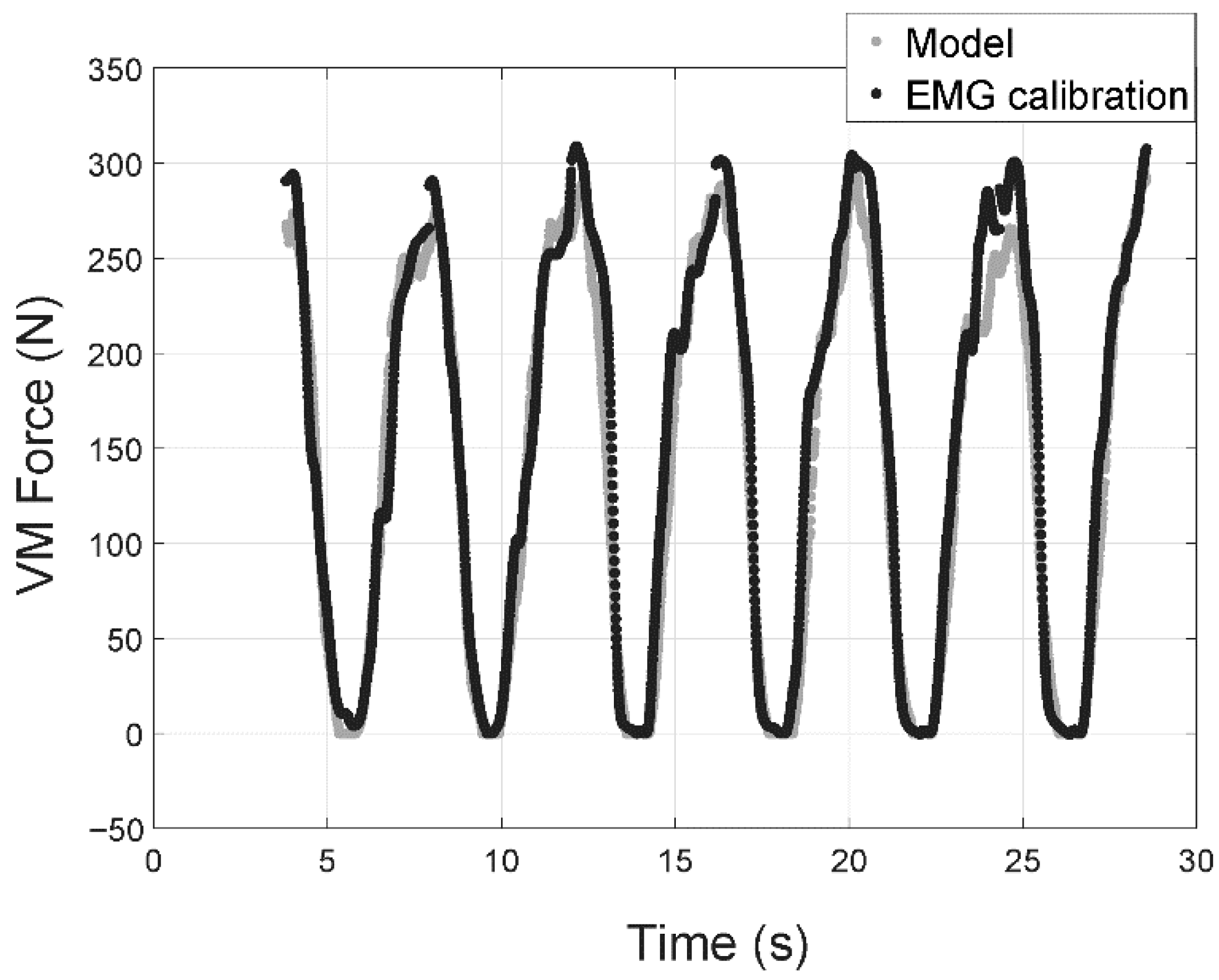
Estimates computed for payload = 6 kg; Force–EMG calibration curves based on payload = 0 and 12 kg trials. ICC: intraclass correlation coefficient. SEM: standard error of measurement.

presents the agreement between the estimated muscle forces using the SGM and the estimation of the same forces obtained by the Force–EMG calibration curves. These calibration curves were obtained for each subject based on data (estimated muscle forces—measured EMG signals) from two load conditions: L0 and L2. These curves were used to estimate the forces from the EMG signals and in the exercise with L1 load condition.

These results provide an excellent correspondence between the model-based estimated forces and those obtained based on Force–EMG calibration. The mean ICC values were higher than 0.96 for both muscles and both directions of motion of the knee. The 25th percentile is greater than 0.9 in all cases. With respect to the error level, the mean error was in the order of 5.5% of the force range, while in 75% of cases it was lower than 8%.

Figure 5 displays an example (subject # 3) with excellent correspondence between the results of the model and those obtained from the EMG signals. Both signals are perfectly synchronized, and the differences are very small and are limited to motion extremes.

Table 6. The correspondence between the reaction force on the tibial plateau as measured directly [26], and as estimated using SGM.

	ICC	SEM (% of the Force Range)
Normal compressive force	0.945	5.6
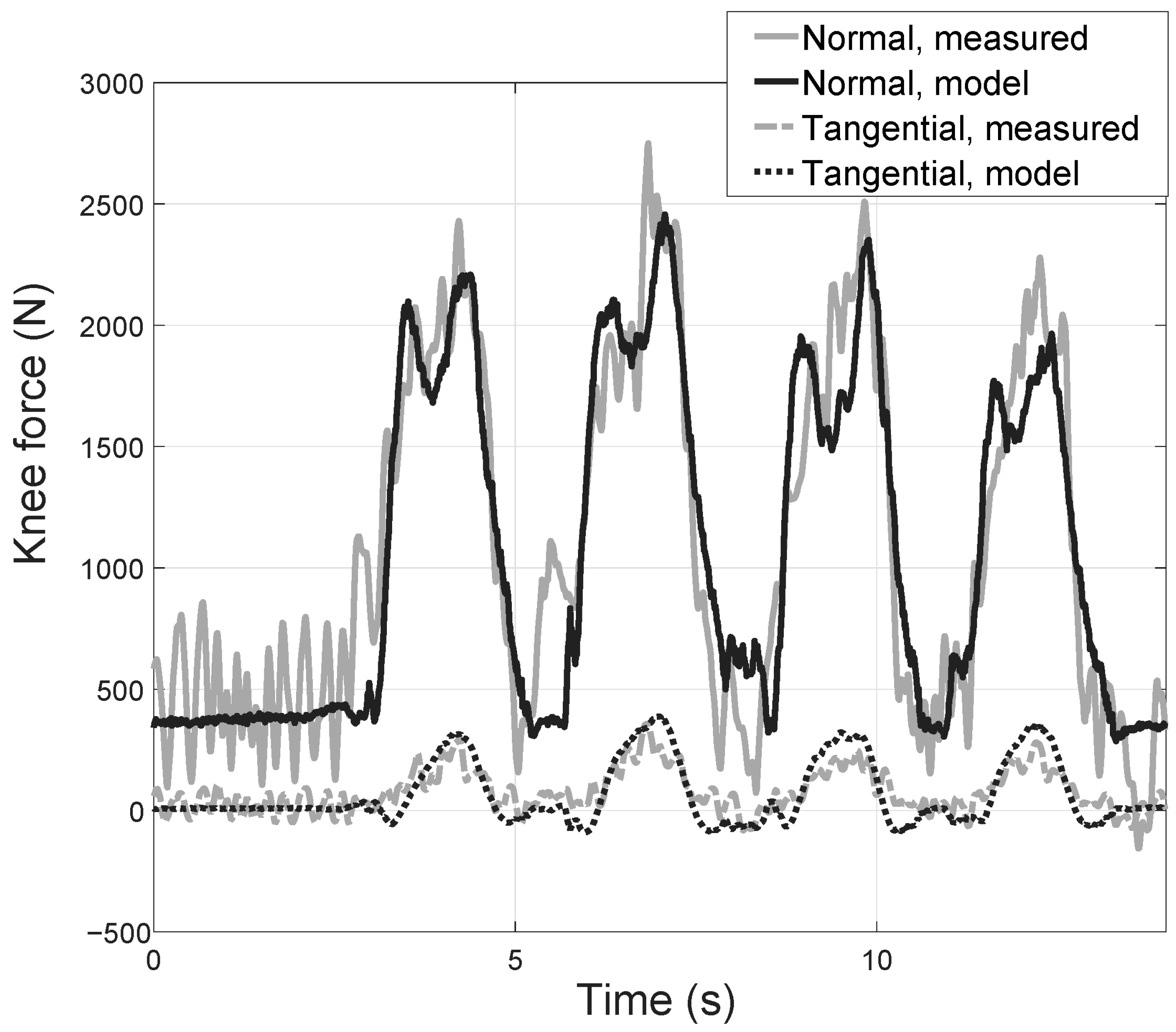
Tangential force	0.827	10.1

shows the results of agreement between the reaction forces in the directions normal and tangential to the tibial plateau as estimated by the quasistatic model, and as measured directly using an instrumented prosthesis [26]. As can be observed, the ICC value is very high for the normal force (0.945), with an error in the order of 6% of the total range. With respect to the force in the tangential direction, the ICC had a worse but still acceptable value (0.827). In this case, the error was in the order of 10% of the total range of this force, which is also small.

Figure 6 presents the measured and estimated forces. As can be observed, the directly measured force has high noise, especially at the beginning of the motion. This noise was smoothed before calculating the agreement parameters (Figure 6 shows the raw signal). As can be seen, despite this noise, the correspondence between the reaction forces (in the normal and tangential directions) is good: measured and estimated forces are in-phase, and had similar amplitudes.

The computation time required to calculate the forces in a cycle of calculation for a leg configuration is less than 2.51 ms using a Personal Computer with Ram Intel Core i7-8700K 32 Gb, SUSTek PRIME B360M-A Rev X.0x Motherboard and Matlab R2020b, which allows its integration into a rehabilitation robot control system. This is because, in the control system, a real time system programmed in C++ will be used.

4. Discussion

RPRs need to be assisted by MSMs that provide estimates of internal efforts, both for safety reasons and to ensure the effectiveness of rehabilitation exercises. Although there is extensive research activity in the field of MSMs, current approaches are directed towards greater complexity and levels of anatomical and physiological detail or the incorporation of information on muscle activity measured by EMG [15]. Despite their scientific interest, they are complex and expensive models in terms of time and equipment, which limits their applications in clinical practice and in the control of RPRs.

MSMs used for controlling RPRs must be adaptable to the patient’s characteristics, simple, and able to operate in real time, while also providing accurate estimates of the muscle forces and identifying overexertion in the body structures. In this paper, we present a model based on essential actions that attempt to solve some of the applicability problems of the current models. The level of detail used is like that of other previous models [15,43]. However, some improvements were introduced to accomplish the aforementioned requirements.

First, the kinematics of the knee joint is customized by adjusting a four-bar mechanism. This simplified model offers better results than those based on a fixed axis of rotation, without the need-to-know anatomical details, such as models that use the characteristics of the ligaments. The adjustment is carried out using a functional calibration process, which provides an advantage over parametric models obtained with specimens [10].

This aspect is relevant in the case of clinical applications, where it is important to be able to adapt the joint model to specific rehabilitation movements performed by people with medical disorders, and thus altered movement patterns [4,5,6,7,8,9,10,11].

Secondly, simplifications have been made to the inverse dynamics model to reduce calculations and allow a real-time estimation of internal forces. This is necessary for effective control of the robot. For this, a quasistatic model is used, not considering the inertial forces compared to the segment weights and those directly applied. This simplification has two consequences. First, it makes the numerical calculation of velocities and accelerations unnecessary and, secondly, it transforms the relationships between forces and joint moments into geometric relationships that only depend on position. This allows the optimization process, used to solve muscle force indeterminacy problem, to have a direct analytical solution using Lagrange multipliers. As a result, muscle coefficients can be calculated in an offline calibration stage. The calculations of the muscle coefficients associated with an exercise can be reduced by assuming one functional degree of freedom [8,41]. Then, the manifold combinations associated with fDOFs are much fewer than those corresponding to kinematic DOFs, which reduces the computational time and simplifies the application of the model.

Another relevant aspect in the development of an MSM is its verification and validation. The verification and validation of the model have been carried out through the analysis of the squat movement, using a conventional biomechanical laboratory [2]. Regarding the movement used, it is an easily reproducible gesture that causes significant efforts at muscle and joint level. It has already been used previously in other works [5].

Although there are some guidelines on the MSM validation strategy, most of the published papers only verify the coherence between the estimated forces and the EMG signals. However, validation in a physical sense involves comparing estimated and measured forces directly. In this paper, we have followed this double strategy. First, the coherence between the EMG signals and the estimated forces was verified with calibration curves obtained in independent exercises. This strategy has been suggested previously [24], and ensures that the validation data are independent of those used in the calibration curves. Secondly, a direct validation was made with experimental measures [26].

The experimental results demonstrated the validity of the hypotheses of our simplified model. Thus, in all cases, the variance explained by the knee angle was very high (lower quartile 98.5%), which confirms the hypothesis that there is a single fDOF. Therefore, all generalized coordinates could be predicted accurately from one main variable (knee flexion in this movement). This result has already been verified in other joints when cyclical repetitions are performed [42].

Regarding the hypothesis of the quasistatic regime, there is a practically perfect correspondence between the estimates associated with the FDM and SGM models. Thus, the ICC between both models is higher than 0.999, with errors lower than 0.1% of the joint moment range. This shows that, in slow movements such as those usually applied in rehabilitation, the inertial forces are negligible.

The coherence between the estimated forces and the EMG signals in the active muscles (vastus lateralis and vastus medialis) is significant. The correlation coefficients were greater than 0.931 in all cases. Furthermore, the correspondence between the forces estimated by the model and those obtained by the Force–EMG calibration curves was also very good, with ICC values higher than 0.966 and an SEM of the order of 5% of the range. Note that this verification was performed with different exercises than those used to obtain the calibration curves. Although this validation is indirect, since the forces in the tendons have not been measured, it shows that the model is consistent with the levels of muscle activation.

Finally, the correspondence between the estimates of the joint forces of the model and those measured experimentally in the SGM has also been verified. The ICC obtained for the compression force is 0.945, with an error of 6% over the range of the registered force. For tangential forces, the result was somewhat worse, but in any case, very good, with an ICC of 0.827 and an error of 10% of the range. Obviously, the results obtained in the direct validation correspond to a single subject, and we should expand the sample to include other subjects and exercises. However, the results of this work confirm that assuming the appropriate hypotheses and adjusting the model to the essential muscles, it is possible to obtain a very simple model capable of offering estimates that are consistent with muscle activity and in vivo measurements of joint forces. Moreover, the stationary geometric approach used is compatible with performing offline calculations, which will help provide efficient models that are capable of operating in real time. These are essential requirements for its use in the control of rehabilitation robots.

5. Conclusions

A highly recommended feature in rehabilitation robots is that the control system has access to a real time estimate of force in muscles and ligaments. Having this capacity significantly increases patient safety, and it allows the practitioner to obtain precise data on the evolution of the rehabilitation process. For this reason, it is essential to have musculoskeletal models which are adaptable to the characteristics of the patient, offering valid estimates and operating in real time. Advances in recent years have been directed towards the development of very complex models that use a large number of parameters, and are computationally expensive. Furthermore, there are important problems for the experimental validation of such models.

The simplification of the models without losing predictive capability should be oriented fundamentally in two directions: on the one hand, personalizing the joint kinematics to obtain a good representation of the individual movement and, on the other, eliminating those actions that do not contribute significantly to the movement.

In this research, a simple model is proposed, which allows a sufficient level of individual adaptation and simple calculations that can be performed in real time. For this, a kinematic calibration is carried out, and a rescaling model based on anatomical markers is used, which allows a good adaptation to the anatomical characteristics and the movement pattern of each patient. Furthermore, dynamic calculations are simplified by eliminating inertial actions, which have no appreciable effect on joint torques. Finally, an offline optimization procedure is used, which allows for uncoupling the calculations from the biomechanical model during robot operation. This procedure uses the concept of functional degree of freedom, which makes it possible to reduce the dimensionality in the optimization process, constraining the calculations to a band of combinations of kinematic variables of reduced dimensionality.

The validity of the hypotheses, the coherence between the estimates of the model and the levels of muscle activity measured with surface electromyography have been verified. In addition, estimates of joint forces have been compared with those measured directly using an instrumented knee prosthesis, based on data published in the Grand Challenge Competition to Predict In Vivo Knee Loads.

In summary, the proposed model incorporates the essential characteristics that allow an excellent personalization to obtain reasonable estimates of the internal forces through a simple model and with a low computational cost. These are the fundamental characteristics for the use of MSM models for real-time control of rehabilitation robots.