Dynamics of Submersion of a «Diving Buoy» with Account of Hull Compression and Depth-Wise Variation of Water Density

Abstract

The paper employs a simplified approach to modeling of dynamics of submersion of a «diving buoy» subject to a depth-wise water density gradient and experiencing compression of the hull due to action of pressure. The latter effect is accounted for through use of well-known boiler formulae of structural mechanics allowing to analyze behavior of hulls made of different materials. Operation of a piston type buoyancy engine is modeled both for a hypothetical case of instantaneous change of buoyancy and for more practical case of finite buoyancy variation. As the analysis includes both acceleration/deceleration and constant speed modes of motion it enables to evaluate full time of submersion to a design depth. Calculated are the vertical position and speed of the vehicle versus time. Due to the fact that during submersion the growth of density results in deceleration and hull compression causes acceleration, the equilibrium condition is formulated which can be seen as hanging mode in which the buoy performs damped oscillations around a depth of hanging with a frequency depending on rates of density and compression. It is shown that to provide constant speed for a general case of density variation one has to secure a corresponding volume variation of the vehicle or a corresponding increment/decrement of differential buoyancy. At the end of the paper estimates are presented showing how much additional buoyancy should be carried on board to keep constant speed of submersion and how much power is needed for corresponding buoyancy control for a given density profile.

1. Introduction

Diving buoys (DB) [1,2,3] and underwater gliders (UG) [4,5,6,7,8,9,10] have become well-established economical instruments of ocean exploration both for use as separate devices and in swarms vastly extending our capacity to provide efficient spacial-temporal monitoring of water basins. Chronologically the UGs originated from the DBs through addition of lifting elements which secure horizontal component of motion.

One of the problems attracting attention of engineers who develop DBs and UGs in the large range of depths is buoyancy control which requires account of various factors, and, in the first place, those of depth-wise density gradient and pressure hull compression. One needs to emphasize that these issues are important to retain most valuable quality of a properly designed underwater glider- low expense of energy. Sometimes, neglecting the issue of buoyancy control would result in difficulties on the way to conquering the depth. Enough to recall that reaching the bottom of Marianna trench required use of dedicated thrusters for James Cameron’s Challenger venture, [11].

Note that dynamics of diving buoys (profilers) and underwater gliders along with their buoyancy engines as well as corresponding energy consumption modeling have been discussed in several preceding papers. Reference [12] reported details on construction of a buoyancy engine for an underwater glider design challenge being to build a vertically translating programmable buoyancy engine capable of diving to the depth of 20 m.

It is emphasized in [13] that in the «depth-varying oceanic environment, the buoyancy of deep-sea underwater gliders (UGs) will change with depth due to pressure hull deformation and seawater density variation. As the buoyancy variation caused by these two factors is of the same order of magnitude as the nominal net buoyancy, hull deformation and seawater density variation will accordingly affect the dynamic behaviors of deep-sea UGs». Comparison of simulated results obtained with account of density gradient and hull compressibility with a simpler mathematical model not accounting for these properties and sea trials showed that hull deformation and sea water density variation have considerable effect on pitch angle and velocity of the gliders. Ensuing from this analysis was a proposed buoyancy compensation scheme validated to be effective in the course of sea trials.

It is underlined in [14] that full assessment of the energy loss due to the hull and water compressibility effects is very important in view of necessity of using thus saved UG battery power for indispensable additional instrumentation, such, for example, as Doppler velocity logger, and, in any case, for extended range capability for a given battery power. This power-saving vector of the UG development would bring along various improvements including hydrodynamic optimization of the hull and lifting system and energy harvesting capacity of the vehicle.

The authors of [15] comment that variation of sea water density and hull compressibility affects driving buoyancy of the UG, resulting in unstable motion, and propose a novel hybrid passive buoyancy compensation system based on three standalone systems with the goal to reduce buoyancy change.

Buoyancy control issues are closely interrelated with the problem of energy consumption modeling (ECM) for underwater gliders. Paper [16] deals with ECM and states that such modeling is indispensable for efficient energy management of the UG as well as for their safe operation. This paper sets forth a comprehensive ECM of UGs which comprises consideration of ocean currents, seawater density variation, deformation of the pressure hull and asymmetry of gliding motion during descending and ascending. Sea trial data used by the authors shows that account of the currents brings about a significantly higher accuracy of the ECM. The paper also reveals how energy consumption relates to multiple parameters of the UG such as gliding velocity with respect to the current and diving depth.

Note, that the buoyancy loss due to seawater and hull compressibility has been studied in [13,15].

It is worth mentioning that an important feature of the ocean is stratification. Whereas here we restrict ourselves to the case of continuous variation of density there exist practical situations when the density has a step change. This can be exemplified by layers of fresh water contained between salted (sea) water and ice fields which can extend to several tens of meters depth-wise. The latter layer is formed due to ice melting into the sea. It can be easily demonstrated that, in spite of relatively small difference of the order of 2.5% between densities of sea and fresh water, the ascending UG cannot overcome this interface, enters into a hanging mode and may perform damped oscillations with frequency depending on relative difference of fresh and sea water densities.

Some recent papers also discuss neutral buoyancy hulls which ensure possibility of depth-wise station keeping modes of operation which are known to have been widely employed for drifting buoys. One of the options is related to use of optimal neutrally- buoyant pressure hulls [17]. Discussed in [18] is flexible-bodied UG with neutral buoyancy so named Flexible-Liquid-Rigid (FLR) composite hull.

Note that with purpose of buoyancy control of the diving buoys simplified engineering approaches are presented in [19] and [20] where in the authors state that the accuracy of measuring of physical parameters of water essentially depends on the speed of vertical motion of the diving buoys. In these papers variation of water density and hull deformation were not accounted for. The estimates have been made by the authors of the time for ascension and submersion in what they call ordinary and energy-saving modes.

The motivation for preparing this paper was to construct a simple mathematical model that would allow to assess main effects related to water density variation and hull compression and explore influence of corresponding buoyancy control. To simplify the model we are using one-dimensional formulation reducing mathematics to an ordinary differential equation including terms accounting for depth-wise density gradient in combination with elementary boiler formulae of structural mechanics for hull compression. The latter enable evaluation of the influence of the pressure hull geometry and material on the dynamics of submersion. Further glider applications would require consideration of lifting appendages (wings) although hopefully the effects in question would mostly depend on the depth effects studied herein for purely vertical motion. Advantages in applying a simplified model similar to what is discussed hereinafter include a possibility to explore energy expense required for compensation of buoyancy variation exemplified for the case of securing constant speed of submersion for a vehicle subject to influence of vertical density gradient and hull deformation. The present approach also allows to explore plausibility of an evident suggestion of counterbalancing nature of the accelerating effect of hull compression and decelerating impact of density growth (pycnocline effect). The model in question naturally produces a requirement of equal rate of compression of water and pressure hull as a condition of constant speed and easily yields a provision leading to hanging modes whereby the vehicle stops and can be moved further through buoyancy control on board.

In what follows: we formulate one dimensional mathematical description of the problem, then discuss analytical and numerical solutions for the speed and depth of submersion, exemplified by cylindrical and spherical pressure hulls with and without account of density gradient and hull compression. When the latter effects are present we explore conditions of occurrence of hanging modes of the vehicle as well as buoyancy control for provision of constant speed of vertical motion with estimates of required energy expense and on-board buoyancy reserve.

2. Mathematical Model

Let a body (pressure hull) perform its descent along its axis of revolution and in the direction of positive $z$. Therewith, the equation of the motion of the body takes the form

$$(M+m^{\prime })\ddot{z}(t)=Mg-\rho (z)gV(t)-C_D\frac{\rho (z)}{2}{S}_D\dot{z}(t)|\dot{z}(z)|.$$

(1)

Equation (1) comprises the following notations: $M$ is the mass of the body; $m^{\prime }$ is the added mass of water in the direction of motion; $g$ is the gravitational acceleration; $\rho (z)$ is the water density at depth $z$; $V(t)$ is the variable volume of the pressure hull; $C_D$ is the hydrodynamic drag coefficient of the body in axial flow with reference to the maximum area of its lateral cross-section $S_D$; $z(t)$ and $\dot{z}(t)$ are the submersion and speed of the body correspondingly.

Note that Equation (1) implies the quadratic law of hydrodynamic drag. Representing the volume of the pressure hull as $V(t)=V_0-\Delta V_c(z)\mp \Delta V_b(t)$, where $V_0$ is the volume of the pressure hull in the state of neutral buoyancy prior to submersion $({\rho }_0{V}_0=M)$, $\Delta V_c(z)$ is the variation in the volume of the body due to its compression under the action of pressure at depth and $\Delta V_b(t)$ is the variation in buoyancy, one can reduce Equation (1) to

$$\ddot{z}(t)=\frac{1}{1+\lambda }\{g[1-\frac{\rho (z)}{{\rho }_0}[1-\frac{\Delta V_c(z)}{V_0}\mp \frac{\Delta V_b(t)}{V_0}]]-C_D\frac{\rho (z)}{2{\rho }_0}\frac{S_D}{V_0}\dot{z}(t)|\dot{z}(t)|\},$$

(2)

where $\lambda =m^{\prime }/M$, and ${\rho }_0$ is the density of water near the surface. Introducing the relative density $\overline{\rho }(z)=\rho (z)/{\rho }_0$, relative compression of the body ${\eta }_c(z)=\Delta V_c(z)/V_0$ and relative maximal volume of replacement $\eta =\Delta V_0/V_0$, re-write Equation (2) as follows

$$\ddot{z}(t)=\frac{1}{1+\lambda }\{g[1-\overline{\rho }(z)(1-{\eta }_c(z)\mp \eta \cdot f(t))]-C_D\frac{\overline{\rho }(z)}{2l^{*}}\dot{z}(t)|\dot{z}(t)|\},$$

(3)

where $f(t)$ is the normalized function of time defined for the period of the buoyancy change; $l^{*}$ is the ratio of the body volume to its maximal lateral cross-sectional area $(l^{*}=V_0/S_D)$. The solution of Equation (3) with appropriate initial conditions and control function $f(t)$ allows finding parameters of the vehicle’s submersion accounting for the regimes of acceleration, steady motion and deceleration motion, depth-wise variation in physical characteristics of water, configuration and dimensions of the body, as well as compression of the body under the action of pressure.

3. Analytical and Numerical Solutions

3.1. Case of Constant Density and Incompressible Hull

Consider first the case of depth-wise constant density $\rho (z)\equiv {\rho }_0$ and incompressible pressure hull $\Delta V_c(z)\equiv 0$. Therewith, Equation (3) takes the form

$$\ddot{z}(t)=\frac{1}{1+\lambda }[g\eta \cdot f(t)-\frac{C_D}{2l^{*}}\dot{z}(t)|\dot{z}(t)|];z(0)=0,\dot{z}(0)=0,$$

(4)

At the first stage, separately consider the processes of acceleration and deceleration of the body. Assume that it begins submersion from the free surface from the state of equilibrium. Then, the problem for accelerated submersion takes the form

$$\ddot{z}(t)=\frac{1}{1+\lambda }[g\eta \cdot f_a(t)-\frac{C_D}{2l^{*}}{\dot{z}}^2(t)];z(0)=0,\dot{z}(0)=0,$$

(5)

where the function $f(t)$ at acceleration is adopted in the form $f_a(t)=t/t_0$ for $t\le t_0$ and $f_a(t)=1$ for $t\ge t_0$, and $t_0$ is the time of the buoyancy change. The acceleration of the body will continue until the moment it becomes equal to zero. Assuming that after this moment, $t\ge t_0,f(t)=1$, we obtain the speed ${\mathrm{v}}_{\mathrm{s}}$ at the beginning of the steady motion phase

$${\mathrm{v}}_{\mathrm{s}}=\sqrt{\frac{2g{l}^{*}\eta }{C_D}}.$$

(6)

It follows from Equation (6) that for a given body, the speed of submersion during the stationary stage of motion is proportional to the square root from the relative volume of replacement. On the other hand, if the latter quantity is fixed, the speed of stationary submersion is proportional to the square root of the ratio $l^{*}/C_D.$ Assuming the buoyancy change is instantaneous $(t_0=0)$, Equation (5) can be integrated in closed form. The dependences of the speed of submersion and vertical distance from the free surface were obtained in the form

$$\dot{z}(t)=\sqrt{\frac{2g{l}^{*}\eta }{C_D}}\tanh \left(\sqrt{\frac{g\eta C_D}{2l^{*}}}\frac{t}{(1+\lambda )}\right)$$

(7)

$$z(t)=\frac{2l^{*}(1+\lambda )}{C_D}\ln \cosh \left(\sqrt{\frac{g\eta C_D}{2l^{*}}}\frac{t}{(1+\lambda )}\right).$$

(8)

To approximately determine the moment of time when the body motion becomes steady, solve Equation (7) with respect to time

$$t=(1+\lambda )\sqrt{\frac{2l^{*}}{g\eta C_D}}{\tanh }^{-1}\left(\frac{\dot{z}}{{\mathrm{v}}_{\mathrm{s}}}\right).$$

(9)

where is defined by the formula (6). Denote as $t_a$ the time of completion of accelerated submersion when the magnitude of speed constitutes 0.99 of the maximum speed. Then,

$$t_a=(1+\lambda )\sqrt{\frac{2l^{*}}{g\eta C_D}}{\tanh }^{-1}(0.99)\cong 2.65(1+\lambda )\sqrt{\frac{2l^{*}}{g\eta C_D}}.$$

(10)

The distance covered by that moment of time, determined with the same accuracy, can be found by means of the formula

$$z_{ma}=\frac{2l^{*}(1+\lambda )}{C_D}\ln \cosh [{\tanh }^{-1}\frac{\dot{z}(t_{ma})}{{\mathrm{v}}_{\mathrm{s}}}]=\frac{2l^{*}(1+\lambda )}{C_D}\ln \cosh ({\tanh }^{-1}(0.99))\cong 3.92\frac{l^{*}(1+\lambda )}{C_D}.$$

(11)

As follows from equation (11), the quantity $z_{ma}$ does not depend on the volume of replacement. In Figure 1, Figure 2, Figure 3 and Figure 4, the results obtained by means of Equations (7) and (8) are presented for the case of an elongated cylinder ($l^{*}=l_c,l_c/d_c={\kappa }_c=10,$$l_c=1$ m, $C_D=0.82$, ${\lambda }_c<<1$) and a sphere of identical volume.

$$(d_s=l_c{(3{\kappa }_c{}^2/2)}^{1/3}\cong l_c/4,l^{*}=2d_s/3,C_D=0.4,{\lambda }_s=0.5)$$

It was assumed above that the buoyancy change takes place instantaneously. In reality, the buoyancy change occurs during a finite interval of time $t_0$. Some results of the numerical solution of the acceleration problem shown in Equation (5) for the cylinder assuming the linear law of the buoyancy change are presented in Figure 5 and Figure 6.

It was assumed above that the buoyancy change takes place instantaneously. In reality the buoyancy change occurs during a finite interval of time $t_0$. Some results of numerical solution of the acceleration problem (5) for the cylinder on assumption of linear law of the buoyancy change are presented in Figure 5 and Figure 6.

Numerically found solutions of the Equations (7) and (8) are plotted in Figure 5 and Figure 6 with dashed lines. Depending of a given depth corridor $H$ and with account of the body inertia, it is necessary to switch the buoyancy engine to ascension at a certain moment of time $t_{as}$. Therewith starts the process of deceleration of the vehicle until it stops completely.

Consider first the analytical description of the deceleration process for the case of an instantaneous $(t_0=0)$ relative buoyancy change from $-\eta$ to $\eta$. Accordingly, the problem acquires the form

$$\ddot{z}(t)=-\frac{1}{1+\lambda }[g\eta +\frac{C_D}{2l^{*}}{\dot{z}}^2(t)];z(0)=0,\dot{z}(0)={\mathrm{v}}_{\mathrm{s}}.$$

(12)

Note that in Equation (12), the time is counted from the moment of the start of deceleration. Integrating Equation (12) with initial conditions, we obtain the following expressions for instantaneous speed of deceleration and the distance covered from the start of deceleration until the vehicle completely stops in the form

$$\dot{z}(t)={\mathrm{v}}_{\mathrm{s}}\tan \left(\frac{\pi }{4}-\sqrt{\frac{g\eta C_D}{2l^{*}}}\frac{t}{(1+\lambda )}\right)$$

(13)

$$z(t)=\frac{2l^{*}(1+\lambda )}{C_D}\ln [\sqrt{2}\cos (\frac{\pi }{4}-\sqrt{\frac{g\eta C_D}{2l^{*}}}\frac{t}{(1+\lambda )})].$$

(14)

As seen from Equation (13), the vehicle completely stops at the moment of time

$$t=t_d=\frac{\pi (1+\lambda )}{4}\sqrt{\frac{2l^{*}}{g\eta C_D}}.$$

(15)

Substituting Equation (15) into Equation (14), we obtain the deceleration distance

$$z_{md}=z(t_d)=\frac{2l^{*}(1+\lambda )}{C_D}\ln \sqrt{2}.$$

(16)

It follows from Equation (16) that the deceleration distance as well as acceleration distance—see Equation (11)—do not depend on the relative volume of replacement. After the time moment $t=t_d$, the vehicle starts to ascend. For a description of the acceleration in ascending motion, it is necessary to consider the corresponding equation

$$\ddot{z}(t)=-\frac{1}{1+\lambda }[g\eta -\frac{C_D}{2l^{*}}{\dot{z}}^2(t)]$$

(17)

with initial conditions $z(t_d)=z_{md}$, $\dot{z}(t_d)=0$. The solution of Equation (17) taking account of initial conditions was found in the form:

$$\mathrm{z} \dot{} \left(\mathrm{t}\right)={-\mathrm{v}}_{\mathrm{s}}\tanh (\sqrt{\frac{g\eta C_D}{2l^{*}}}\frac{t}{(1+\lambda )}-\frac{\pi }{4})$$

(18)

$$z(t)=\frac{2l^{*}}{C_D}\ln \frac{\sqrt{2}}{\cosh (\sqrt{\frac{g\eta C_D}{2l^{*}}}-\frac{\pi }{4})}.$$

(19)

The calculation of the process of deceleration for the case of an instantaneous change in buoyancy on the basis of an analytical solution taking account of the vehicle’s full stop and the subsequently accelerated ascension is presented in Figure 7 and Figure 8 for the case of the cylinder and in Figure 9 and Figure 10 for a sphere of identical volume.

The analytical results obtained for the deceleration process are valid on the assumption of an instantaneous change in relative buoyancy from $-\eta$ to $\eta$. The finiteness of the time of the buoyancy change can be made through the numerical solution:

$$\ddot{z}(t)=\frac{1}{1+\lambda }[g\eta \cdot f_d(t)-\frac{C_D}{2l^{*}}\dot{z}(t)|\dot{z}(t)|];z(0)=0,\dot{z}(0)={\mathrm{v}}_{\mathrm{s}},$$

(20)

where the control was adopted in the form $f_d(t)=1-t/t_0$ for $0\le t\le 2t_0^{}$ and $f_{da}(t)=-1$ for $t\ge 2t_0$, allowing accelerated ascension after the vehicle completely stops. In Figure 11 and Figure 12 are calculated data characterizing the influence of finiteness of time of the buoyancy change upon the process of deceleration and subsequent ascension of the cylinder.

The results obtained above enable estimating the full time of submersion $t_{\Sigma }$. Summed up therewith are the time of acceleration, time of steady motion and time of deceleration until complete stop. The time of acceleration $t_a$ and deceleration $t_d$ are determined through Formulae (10) and (15), and the time of steady submersion is determined by means of the formula

$$t_s=\frac{H-z_{ma}-z_{md}}{{\mathrm{v}}_{\mathrm{s}}}$$

(21)

where $z_{ma}$ и $z_{md}$ are the lengths of acceleration and deceleration distances. The calculated data are presented in

Table 1. Dependence of the full time of submersion of the cylinder on the change in relative volume of replacement for $H=200\mathrm{m}$, $l=2\mathrm{m}$, $t_0=20\mathrm{s}$.

$\mathit{\eta }$	${\mathit{t}}_{\mathit{a}}[\mathbf{s}]$	${\mathit{z}}_{\mathit{m}\mathit{a}}[\mathbf{m}]$	${\mathit{v}}_{\mathit{s}}[\mathbf{m}/\mathbf{s}]$	${\mathit{t}}_{\mathit{d}}[\mathbf{s}]$	${\mathit{z}}_{\mathit{m}\mathit{d}}[\mathbf{m}]$	${\mathit{t}}_{\mathit{s}}[\mathbf{s}]$	${\mathit{t}}_{\mathit{\Sigma }}[\mathbf{s}]/[\mathbf{min}]$
0.001	29.7	1.5	0.21	41.4	5.83	917	988/16
0.005	28.4	6.3	0.49	43.2	10.2	375	447/7.5
0.01	27.5	9.8	0.69	30.2	13.2	257	315/5.2
0.02	25.1	13.1	0.98	28.1	17.3	173	226/3.8
0.03	23.7	15.4	1.2	27.0	20.4	137	188/3.1
0.05	22.4	19.0	1.55	26.0	25.2	100	148/2.5

for the case of a cylinder with length $l_c=2$ m. The full time of submersion is given in the last column of Table in seconds and minutes (in bold font).

The full submersion time was also calculated by means of the direct numerical solution in Equation (20). Used therewith was the control function $f(t)$, defined in the following way:

for $t\le t_{as}$,

$$f(t)=\{\begin{array}{l}t/t_0,t\le t_0;\\ 1,t\ge t_0.\end{array}$$

(22)

for $t\ge t_{as}$,

$$f(t)=\{\begin{array}{l}1-(t-t_{as})/t_0,t_{as}\le t\le t_{as}+2t_0;\\ -1,t\ge t_{as}+2t_0,\end{array}$$

(23)

where $t_{as}$ is the moment of time to turn on the BE for deceleration until completely stopping and starting ascension.

Such calculation was carried out for the case of submerging the cylinder of length $l_c=1 \mathrm{m}$ and values of $\eta =0.001,0.005,0.01,0.02,0.03,0.05$. The value of $t_{as}$ was defined as a sum of $t_a$ and $t_s$ for corresponding values of $\eta$ from Table 1. The dependencies of submersion $z(t)$ and speed of submersion $\dot{z}(t)$ on time for $\eta =0.005$ are presented in Figure 13 and Figure 14. Function $f_{as}(t)$ is shown in Figure 14 with a dashed line.

In the course of calculations, the full time of submergence, which for all values of $\eta$ listed in Table 1 was practically indistinguishable from $t_{\Sigma }$, was determined.

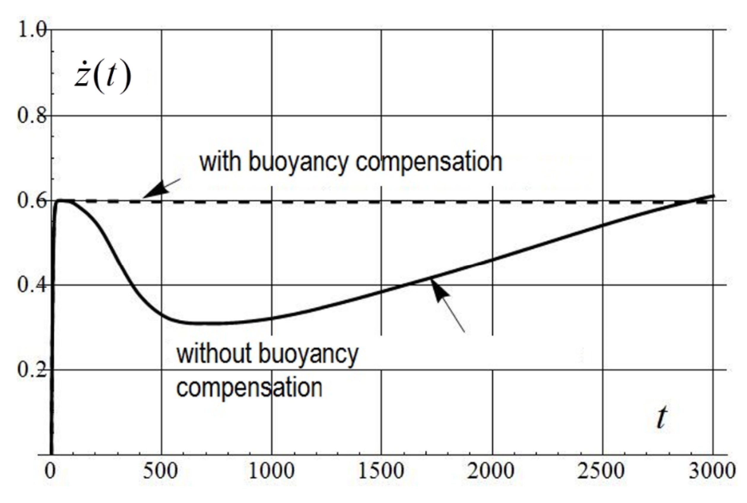
3.2. Case of Variable Density and Compressible Hull

Here, we perform a simplified analysis of submersion of a body equipped with BE considering depth-wise variation in density and hull compression. Depth-wise density distribution can be evaluated through corresponding profiles of temperature, salinity and pressure. In Figure 15 and Figure 16, the typical density profiles for equatorial waters and Northern seas are presented.

Taking account of the hydrostatic law of increase in pressure depth-wise, the linear dependence of the hull compression on $z$ can be

$${\eta }_c(z)=\frac{\Delta V_c(z)}{V_0}={\eta }_{c_{\max }}\cdot \frac{z}{H},$$

(24)

where $H$ is the design maximal depth, and ${\eta }_{c_{\max }}$ is the maximal relative hull compression. Quantity ${\eta }_{c_{\max }}$ can be determined using the well-known boiler formulae of structural mechanics.

For a cylinder,

$${\eta }_{c_{\max }}=\frac{p_H\cdot r_c}{E\cdot {\delta }_c}\left(\frac{5}{2}-2{\nu }_P\right).$$

(25)

For a sphere,

$${\eta }_{c_{\max }}=\frac{3p_H\cdot r_s}{E\cdot {\delta }_s}\left(\frac{1-{\nu }_P}{2}\right).$$

(26)

In Formulas (25) and (26): $p_H$ is the design pressure at depth $H$; $r_c$ and $r_s$ are the radii of the cylinder and the sphere, correspondingly; ${\delta }_c,{\delta }_s$ are the thicknesses of the hull shell for the cylinder and sphere, correspondingly; $E$ is the module of elasticity; ${\nu }_P$ is the Poisson coefficient. It is assumed in this paper that for a given design pressure, the relative thickness of the hull shell is calculated based on yield strength ${\sigma }_T$ using the formula

$$\frac{p_H\cdot r}{\delta }\approx {\sigma }_T.$$

(27)

Some results of calculations for a steel cylinder and steel sphere are presented in Figure 17, Figure 18, Figure 19 and Figure 20.

Note that in the calculations it was assumed that the sphere has initial volume identical to that of the cylinder (equivalent sphere).

It follows from equation of motion show in Equation (2) that, in a general case, there can exist hanging modes for which both acceleration and speed of the vehicle are equal to zero. Assuming in Equation (2) that $\dot{z}=0$, $\ddot{z}=0$ и $f(t)=1$, we obtain the following equation of state of equilibrium of the vehicle.

$$1-\overline{\rho }(z_0)[1-{\eta }_c(z_0)\mp \eta ]=0$$

(28)

where $z_0$ is the depth of hanging, if such a mode is realized, i.e., if there exists a solution to Equation (26). Restricting our analysis by the case of submersion, one comes to the following relationship between the relative (in this case, negative) volume of replacement, density profile and hull compression parameters in hanging mode.

$$\eta =\frac{\Delta \rho (z_0)}{\rho (z_0)}-{\eta }_c(z_0)$$

(29)

where $\Delta \rho (z)=\rho (z)-{\rho }_0$ is the increment of density at depth $z$ with respect to the water density at the free surface ${\rho }_0$.

Formally, it is possible to extract from Equation (27) a quantity $\eta$ = ${\eta }_{\max }^{*}(z_0^{*})$ corresponding to the maximal depth of hanging $z_0^{*}$ for a given density profile and hull compression parameters. The maximal depth of hanging $z_0^{*}$ can be found from the following condition.

$$\frac{d\eta (z_0)}{d{z}_0}=0,\frac{{\rho }_0}{{\rho }^2(z_0^{*})}=\frac{{\eta }_{c_{\max }}}{H}.$$

(30)

To illustrate the hanging mode, in Figure 21 and Figure 22, the corresponding dependences of submersion and its speed versus time for a steel cylinder are shown.

Consider the condition of stability of the hanging mode at a depth $z_0$ in the vicinity of zero speed of vertical motion $\dot{z}=0$, by introducing perturbation of depth equal to $\tilde{z}=z-z_0$, accounting for condition of equilibrium from Equation (29) and neglecting the square of speed ${\dot{z}}^2$, one comes to the following equation of perturbed vertical motion of the vehicle near the point of hanging.

$$\ddot{\tilde{z}}(t)+\Omega \cdot \tilde{z}(t)=0,$$

(31)

where

$$\Omega =\frac{g}{(1+\lambda ){\rho }_0}\{\frac{d\rho }{dz}(z_0)[1-\eta -{\eta }_{c_{}}(z_0)]-\rho (z_0)\frac{d{\eta }_c}{dz}(z_0)\}.$$

(32)

Value $\Omega =0$ corresponds to the boundary of oscillatory stability of the hanging mode. For $\Omega ={\omega }^2>0$, an oscillatory motion with a frequency in the vicinity of the depth of hanging may take place. In Figure 23 and Figure 24 with magnification, the typical oscillatory motions of submersion and speed of submersion around depth $z_0$ with zero speed of submersion (on the basis of Figure 21 and Figure 22 for $t\ge 1000$) are shown.

Given below in Figure 25 and Figure 26 are some results of calculations for the equivalent sphere.

In Figure 27 and Figure 28, some results of the calculations for the Northern seas and a design depth of $H=500$ m are presented. Note that in this case, due to the insignificant variation in density versus depth, the hanging modes do not occur.

From Equation (2), there ensues the following condition of existence of the segment of steady submersion:

$$\frac{\Delta \rho (z)}{\rho (z)}=-\frac{\Delta V_c(z)}{V_0}$$

(33)

which can be formulated as a requirement of equality of hull compression and water compression at any depth less than the design depth. If this condition is fulfilled, the vehicle will be descending with a speed close to that determined in [1] and equals

$${\mathrm{v}}_{\mathrm{s}}=\sqrt{\frac{2g{l}^{*}\eta }{C_D}}.$$

(34)

As the compression is varying linearly with respect to $z$, and the density profile is, generally speaking, a nonlinear function of depth and depends on a given basin, exact compliance with the requirement in Equation (31) is practically not viable. In this connection, for realization of vertical motion with a constant speed, compensational control of buoyancy is needed.

From the above, it is easy to see that at a given depth, the required compensational variation in buoyancy equals

$${\eta }_{add}(z)=\frac{\Delta \rho (z)}{{\rho }_0}(1-\eta )-\frac{\rho (z)}{{\rho }_0}{\eta }_c(z).$$

(35)

In Figure 29 and Figure 30, the submersion and its speed versus time accounting for and not accounting for the compensation of buoyancy depth-wise are presented.

For full-depth submersion to $H$, a reserve of the replacement volume is needed equal to

$$\Delta V_{add}=\frac{V_0}{H}{\displaystyle \underset{0}{\overset{H}{\int }}{\eta }_{add}(z)dz.}$$

(36)

Assuming that compensational variation in the replacement volume at a current depth takes place instantaneously, we evaluate the energy required for compensational control of buoyancy across the entire submersion distance:

$$E_{add}=\frac{V_0}{H}{\displaystyle \underset{0}{\overset{H}{\int }}p(z){\eta }_{add}(z)dz.}$$

(37)

For preliminary estimates of the energy expenditure required for the functioning of the body equipped with the buoyancy engine, it is useful to know what the fraction of energy required for continuous buoyancy control with respect to the energy needed to switch over to ascension at the lowest point of the design depth corridor is. Taking into account that pressure at depth $\mathrm{z}$ can be approximately calculated by hydrostatic law $p(z)\approx {\rho }_{0}gz$ and that the energy necessary to switch over to ascension at the design depth $H$ is equal to $E_H=2p(H)\cdot \Delta V\approx 2g{\rho }_{0}H\eta V_0$, we obtain

$$\frac{E_{add}}{E_H}=\frac{1}{\eta \cdot H^2}{\displaystyle \underset{0}{\overset{H}{\int }}z{\eta }_{add}(z)dz}.$$

(38)

Estimates of the additional power needed for buoyancy control shows that for a steel hull, the ratio $E_{add}/E_H$ can be of the order of 0.25–0.30.

4. Conclusions

In this work a simplified one-dimensional mathematical model is proposed of vertical submersion of a diving buoy (profiler) with simultaneous account of depth-wise variation of water density and pressure hull compression. Derived therewith are some analytical and numerical results exemplified for the cases of submersion and ascension of cylindrical and spherical bodies. The formulation employed herein enables to evaluate full time of submersion/ascension, reveals realization of hanging modes due to counterbalancing effects of water and hull compression. On an assumption of constant density and no hull compression depth-wise a method is proposed of estimation of full time of vertical submersion of a body along its axis of symmetry with determination of contributions of time of acceleration, deceleration and steady submersion. Analytical solutions are derived for the case of instantaneous buoyancy reversal. Calculated data is obtained illustrating the influence of water density profile and hull compression on the process of submersion. Demonstrated is a possibility of securing submersion with constant speed through compensational control of buoyancy across the submersion depth. Presented are formulae enabling estimation of required reserves of buoyancy and energy expense for realization of submersion with constant speed.

The limitations of the presented research are due to: use of restricted class of body geometry (cylinder and sphere) and very approximate approach for evaluation of the drag and compression of the pressure hull.

Future research may include calculations of hydrodynamic characteristics and deformations of the buoys with more detailed account of their geometry and mechanical structure with use of computational mechanics and CFD.

References

1. Simonetti, P.J. SLOCUM: A long Endurance Ocean Profiler Powered by Thermocline Driven Engine. Sea Technol. 1998, 39, 17–21. [Google Scholar]
2. Davis, R.E.; Sherman, J.T.; Dufour, J. Profiling ALACEs and other advances in autonomous subsurface floats. J. Atmos. Ocean. Technol. 2001, 18, 982–993. [Google Scholar] [CrossRef]
3. D’Asaro, E.A. Performance of Autonomous Lagrangian floats. J. Atmos. Ocean. Technol. 2003, 20, 896–911. [Google Scholar] [CrossRef] [Green Version]
4. Sherman, J.; Davis, R.E.; Owens, W.B.; Valdes, J. The autonomous underwater glider “Spray”. IEEE Ocean. Eng. 2001, 26, 437–446. [Google Scholar] [CrossRef] [Green Version]
5. Griffiths, G.; Davis, R.E.; Erickesen, C.C.; Jones, C.P. Autonomous buoyancy driven underwater gliders. In Technology and Applications of Autonomous Underwater Gliders; Taylor & Francis: London, UK, 2002. [Google Scholar]
6. Jenkins, S.A.; Humphreys, D.E.; Sherman, J.; Osse, J.; Jones, C.; Leonard, N.; Graver, J.; Bachmayer, R.; Clem, T.; Carroll, P. Underwater Glider System Study. Scripps Inst. Oceanogr. Tech. Rep. 2003, 53, 6. [Google Scholar]
7. Bachmayer, R.; Leonard, N.E.; Graver, J.G.; Fiorelli, E.; Bhatta, P.; Paley, D. Underwater gliders: Recent developments and future applications. In Proceedings of the 2004 International Symposium on Underwater Technology (IEEE Cat. No.04EX869), Taipei, Taiwan, 20–23 April 2004. [Google Scholar]
8. Jones, C.; Webb, D.; Glenn, S.; Schogield, O.; Kerfoot, J.; Kohut, J.; Aragon, D.; Haldeman, C.; Haskin, T.; Kahl, A.; et al. Slocum Glider-Expanding the Capabilities; UUSR: Moscow, Russia, 2011. [Google Scholar]
9. Rozhdestvensky, K.V. A View on the Development of Underwater Gliders. In Proceedings of the Plenary Presentation at a Society of Underwater Technology Technical Conference, Shanghai, China, 2 September 2013. [Google Scholar]
10. Lee, C.M.; Rudnick, D.L. Chapter Underwater Gliders. In Observing the Oceans in Real Time; Venkatesan, R., Ed.; Springer International Publishing AG: Berlin/Heidelberg, Germany, 2018; 322p. [Google Scholar]
11. Than, K. James Cameron Completes Record-Breaking Mariana Trench Dive. National Geographic News, 25 March 2021. [Google Scholar]
12. Janes, N. Design of a Buoyancy Engine for an Underwater Vehicle; National Research Council of Canada, Institute for Ocean Technology, Laboratory Memorandum LM-2004-12: St. John’s, NL, Canada, 2004. [Google Scholar]
13. Yang, Y.; Liu, Y.; Zhang, H.; Zhang, L. Dynamic modeling and motion control strategy for deep-sea hybrid-driven underwater gliders considering hull deformation and sea water density variation. Ocean Eng. 2017, 143, 66–78. [Google Scholar] [CrossRef]
14. Song, Y.; Ye, H.; Wang, Y.; Niu, W.; Wan, X.; Ma, M. Energy Consumption Modeling for Underwater Gliders Considering Ocean Currents and Sea Water Density Variation. J. Mar. Sci. Eng. 2021, 9, 1164. [Google Scholar] [CrossRef]
15. Zhou, H.; Fu, J.; Liu, C.; Yao, B.; Lian, L. Dynamic modeling and endurance enhancement analysis of deep-sea gliders with a hybrid buoyancy regulating system. Ocean Eng. 2020, 217, 108146. [Google Scholar] [CrossRef]
16. Xie, X.; Wang, Y.; Yang, S.; Luo, C.; Chen, J. An Optimal Buoyancy Compensation System for Deep-sea Gliders based on GA. In Proceedings of the Global Oceans: Singapore-U.S. Gulf Coast, Biloxi, MS, USA, 5–30 October 2020; pp. 1–5. [Google Scholar] [CrossRef]
17. Yang, M.; Yang, S.; Wang, Y.; Liang, Y.; Wang, S.; Zhang, L. Optimization design of neutrally buoyant hull for underwater gliders. J. Ocean. Eng. 2020, 209, 107512. [Google Scholar] [CrossRef]
18. Zhu, Y.; Liu, Y.; Wang, S.; Wang, Y. A Bionic Flexible-bodied Underwater Glider with Neutral Buoyancy. J. Bionic Eng. 2021, 18, 1073–1085. [Google Scholar] [CrossRef]
19. Dologlonyan, A.V.; Sukhov, A.K. Evaluation of immersion/floating time of marine diving buoys with the help of approximate model. Environ. Control. Syst. 2018, 14, 27–32. [Google Scholar] [CrossRef]
20. Krasnodubets, L.A.; Zaburdaev, V.I.; Alchakov, V.V. Control of marine buoys-profilers as a method of enhancing representativeness of thermokhaline measurements. Models of motions. Mar. Hydrophys. J. 2021, 4, 69–79. [Google Scholar]
Figure 1. Submersion of the cylinder versus time in accelerated motion for an instantaneous change in buoyancy ( t 0 = 0 ) and various magnitudes of η , l c = 1 m.
Applsci 12 02651 g001
Figure 2. Speed of submersion of the cylinder versus time in accelerated motion for an instantaneous change in buoyancy ( t 0 = 0 ) and various magnitudes of η , l c = 1 m.
Applsci 12 02651 g002
Figure 3. Submersion of a sphere versus time in accelerated motion for an instantaneous change in buoyancy ( t 0 = 0 ) and various η , ds = 0.25 m.
Applsci 12 02651 g003
Figure 4. Speed of submersion of a sphere versus time in accelerated motion for an instantaneous change in buoyancy ( t 0 = 0 ) for various η , ds = 0.25 m.
Applsci 12 02651 g004
Figure 5. Submersion of the cylinder versus time in accelerated motion for various magnitudes of t 0 , η = 0.01 , l c = 1 m.
Applsci 12 02651 g005
Figure 6. Speed of submersion of the cylinder versus time in accelerated motion and various magnitudes of t 0 , η = 0.01 , l c = 1 m.
Applsci 12 02651 g006
Figure 7. Submersion of the cylinder from the start of deceleration until complete stop considering the subsequent ascension for an instantaneous change in buoyancy ( t 0 = 0 ) from η to η .
Applsci 12 02651 g007
Figure 8. Speed of submersion of the cylinder from the start of deceleration until complete stop considering the subsequent ascension for an instantaneous change in buoyancy ( t 0 = 0 ) from η to η .
Applsci 12 02651 g008
Figure 9. Submersion of a sphere from the start of deceleration until complete stop with the subsequent ascension for an instantaneous change in buoyancy ( t 0 = 0 ) from η to η .
Applsci 12 02651 g009
Figure 10. Speed of submersion of a sphere from the start of deceleration until complete stop considering the subsequent ascension for an instantaneous change in buoyancy ( t 0 = 0 ) from η to η .
Applsci 12 02651 g010
Figure 11. Submersion of the cylinder from the start of deceleration until complete stop accounting for the subsequent ascension for a change in relative buoyancy from η to η and various t 0 , η = 0.01, l c = 1 m.
Applsci 12 02651 g011
Figure 12. Instantaneous speed of the cylinder from the start of deceleration until complete stop accounting for the subsequent ascension for a change in relative buoyancy from η to η and various t 0 , η = 0.01, l c = 1 m.
Applsci 12 02651 g012
Figure 13. Submergence of the cylinder versus time for l c = 1   m , H = 200   m , η = 0.005 , t 0 = 20 c .
Applsci 12 02651 g013
Figure 14. Speed of submergence of the cylinder versus time for l c = 1   m , H = 200   m , η = 0.005 , t 0 = 20 c .
Applsci 12 02651 g014
Figure 15. Typical depth-wise density distribution in equatorial waters.
Applsci 12 02651 g015
Figure 16. Typical depth-wise density distribution in Northern seas.
Applsci 12 02651 g016
Figure 17. Submersion versus time: equatorial waters, steel cylinder l * = l c = 2 ,   C D = 0.82 ,   η = 0.007 .
Applsci 12 02651 g017
Figure 18. Speed of submersion versus time: equatorial waters, steel cylinder, l * = l c = 2 ,   C D = 0.82 ,   η = 0.007 .
Applsci 12 02651 g018
Figure 19. Submersion versus time: equatorial waters, steel sphere C D = 0.4 ,   η = 0.007 .
Applsci 12 02651 g019
Figure 20. Speed of submersion versus time: equatorial waters, steel sphere, l * = l s = 1 / 3 , C D = 0.4 ,   η = 0.007 .
Applsci 12 02651 g020
Figure 21. Submersion versus tine for a steel cylinder in hanging mode: l * = l c = 2 ,   η = 0.005 .
Applsci 12 02651 g021
Figure 22. Speed of submersion versus time for a steel cylinder in hanging mode: l * = l c = 2 , η = 0.005 .
Applsci 12 02651 g022
Figure 23. Illustration of the oscillatory character of the hanging mode: instantaneous position of the body relative to the point of hanging z = z 0 : steel cylinder l * = l c = 2 ,   η = 0.005 ,   t 1000 s.
Applsci 12 02651 g023
Figure 24. Illustration of oscillatory character of the hanging mode: speed of the body relative to z ˙ ( z 0 ) = 0 : steel cylinder, l * = l c = 2 ,   η = 0.005 ,   t 1000 s.
Applsci 12 02651 g024
Figure 25. Submersion versus time: equatorial waters, sphere, l * = l s = 1 / 3 ,   η = 0.005 .
Applsci 12 02651 g025
Figure 26. Speed of submersion versus time: equatorial waters, sphere, l * = l s = 1 / 3 , η = 0.005 .
Applsci 12 02651 g026
Figure 27. Submersion versus time: Northern seas, sphere, l * = l s = 1 / 3 ,   η = 0.005 .
Applsci 12 02651 g027
Figure 28. Speed of submersion versus time: Northern seas, sphere, l * = l s = 1 / 3 ,   η = 0.005 .
Applsci 12 02651 g028
Figure 29. Submersion of the vehicle versus time for the buoyancy-compensated and non-compensated cases: equatorial waters, steel cylinder, l * = l c = 2 ,   η = 0.007 .
Applsci 12 02651 g029
Figure 30. Speed of submersion versus time with and without compensation of the replacement volume: equatorial waters, steel cylinder, l * = l c = 2 ,   η = 0.007 .
Applsci 12 02651 g030