Reliability Analysis of Military Vehicles Based on Censored Failures Data

Abstract

The paper proposes a methodology of reliability testing as applied to vehicles used in military transport systems. After estimating the value of the reliability function using the Kaplan–Meier estimator, reliability models were developed and analysed. The neural model, which achieved the value of the correlation coefficient R exceeding 0.99, was determined to fit the empirical data the best. On the basis of the approximated reliability function of several models, the reliability characteristics of the tested sample of vehicles were determined. Plots of the failure probability density function for all three models had similar courses over a significant part of the function domain. A failure intensity function was also determined, which varied between models. For the exponential and Weibull model, the expected mileage between failures was calculated, which proved impossible for the neural model. The proposed methodology is capable of modelling reliability characteristics based on the observation of an assumed period of the exploitation process of the selected group of military vehicles.

1. Introduction

Modelling and reliability analysis of technical objects should be an important element in the process of technical systems management. Any failure can result in a decrease in the efficiency of production and logistics processes carried out using technical means [1,2]. Modelling of a technical object operation while taking failure prediction into account makes it possible to minimise losses resulting from such failures. In addition, advanced knowledge of reliability should support the planning process for periodic maintenance and spare parts supply. Therefore, in many fields of science and technology, as well as branches of the economy, attempts are made to create models reflecting the real operational processes of exploitation of technical objects and devices [3,4,5].

Effective operation of military transport systems requires a fleet of reliable vehicles. The occurrence of failures to the means of transport during the task almost always results in greater or lesser losses for the entire system. In order to meet the challenges posed to the armed forces and the requirements for the efficient implementation of transport processes, appropriate maintenance, diagnostic and repair systems must be organised. Reliability models are useful tools for forecasting and evaluating the maintenance and repair needs of military vehicles [6,7,8]. Therefore, the development of accurate reliability models is critical to maintaining the assumed readiness and effectiveness of military transport systems.

Research fields dealing with reliability problems are frequently addressed in the scientific literature [9,10,11,12]. In the article [13], a reliability assessment method was developed as a decision support in the selection of a vehicle fleet for a transport company. The developed indicator took into account reliability characteristics such as mileages to the first failure, mileages between failures and the intensity of failures. The authors of the publication [14] presented a method for determining the reliability function using the Kaplan–Meier estimator and a modified Kolmogorov–Smirnov statistical test. The case study consisted of 5 years of data on the driver’s door locks usage for a sample size of 45 rail vehicles. Whereas in the study [15], an analysis of aircraft reliability was carried out. Several reliability models were analysed using statistical tests. The log-normal model proved to be the closest fitting model for the empirical data collected. In the paper [16], a Cox regression model was developed to account for the relationship between operational and maintenance conditions affecting aircraft reliability.

Modelling the reliability of technical objects using artificial neural networks remains the subject of many scientific publications. Xu et al. [17] proposed regression models based on Multilayer Perceptron (MLP) and Radial Basis Function (RBF) networks, which they then implemented to describe and predict the reliability of turbochargers and engines. The standardised roots of mean square error for the analysed objects reached acceptably low values. The authors of the paper [18], on the other hand, developed a model using the Support Vector Regression method combined with genetic algorithms, whose accuracy was an order of magnitude better than the model based on RBF networks for data taken from the publication [17]. In contrast, the Support Vector Machines-based model, when applied to the time series of failure occurrences presented in the paper [19], achieved accuracy similar to MLP and RBF models.

A significant improvement in prediction accuracy occurred for models presented in publications [20,21]. The first was developed as a hybrid of artificial neural networks and genetic algorithms, for which the magnitude of the time series delay was determined using the Shannon entropy. The smallest error, close to zero, for the datasets from the article [17] was obtained by the one presented in the paper [21]. Its design is based on a hybridisation of dynamic weight particle swarm optimisation-based sine map and back propagation neural network.

In publication [22], a reliability prediction model was developed based on a cascade neural network. A sigmoidal hidden layer activation function along with linear output neuron activation was proposed. The model predicted the value of the reliability function for Computerized Numerical Control (CNC) machines depending on the mean time between failures (MTBF) with an accuracy measured through Mean Absolute Percentage Error (MAPE), ranging from 1.56% to 2.53%. An approach based on the use of a three-layer neural network and remanufacturing coefficients is presented in [23]. Reliability indices for the individual components of the technical system were determined based on the average times between failures. The flexibility of artificial neural networks in fitting degradation paths has been highlighted in publications [24,25]. The authors of these studies used MLP supported by a stochastic process [24] and a Weiner process [25]. Validations of both models were performed using simulated data and spindle systems wear data. For the actual data, the mean absolute relative error for all test trials did not exceed 0.13 in [24] and 0.06 in [25].

A much more structurally complex convolutional neural network was developed by the authors of [26]. The proposed model, when validated with data from three power systems, achieved significantly better fitting results than MLP, SVM (Support Vector Machine) and KNN (K-Nearest Neighbors) models.

In Table 1, the models discussed above, which have been tested using turbocharger and engine datasets, as well as models for predicting the reliability of other technical objects, are summarised in chronological order.

Table 1. Neural modelling of reliability—literature review.

Model	Case Study	Results	Paper
Regressive models based on neural networks (MLP and RBF)	Turbocharges in diesel engine (time to failure) Car engines (miles to failure)	Normalized Root Mean Square Error NRMSE = 3.9 × 10−3 (RBF) for turbocharges NRMSE = 1.22 × 10−2 (MLP Gaussian activation) for engines	[17]
Model (GA-SVR) based on Support Vector Regression (SVR) and Genetic Algorithm (GA)	Turbocharges in diesel engine (data from [17])	MAPE = 0.0387% NRMSE = 4 × 10−4	[18]
Neural model with one and two hidden layers	Vehicles (mileage to failure)	Correlation Coefficient R = 0.80 Error = 9%	[27]
Model based on Support Vector Machines (SVM) (time series regression as an alternative to probability distribution models)	Turbocharges in diesel engine Car engines (data from [17])	NRMSE: 2.4 × 10−3 for turbocharges NRMSE = 1.25 × 10−2 for engines	[19]
PSO+SVM (Particle Swarm-optimized Support Vector Machine)	Turbocharges in diesel engine and car engines (data from [17]) Submarine diesel engines	NRMSE = 2.0303 × 10−4 for turbocharges NRMSE = 7.1126 × 10−3 for car engines NRMSE = 2.0305 × 10−4 for submarine engines	[28]
Hybrid model: neural networks and Genetic Algorithm (GA) (Number of lag data calculated using Shannon entropy)	Turbocharges in diesel engine and car engines (data from [17]) Load-haul-dump (LHD) machines	NRMSE = 2.52 × 10−4 for turbocharges NRMSE = 1.195 × 10−2 for engines R2: 0.94–0.99 and NRMSE = 8.36 × 10−3 for LHD machines	[20]
Neural model based on time series data	Control, operating and military systems	R: 0.82–0.99	[29]
Hybrid model based on metaheuristics and neural networks	Validation on simulated data	Values of Reliability Index and probability of failure are the same as those obtained with other methods	[30]
Model SDWPSO-BPNN (hybrid of dynamic weight particle swarm optimisation-based sine map and back propagation neural network)	Turbocharges in diesel engine (data from [17]) and industrial robot systems	NRMSE = 6.9 × 10−5 for turbocharges NRMSE = 2.3 × 10−6 for industrial robot systems	[21]
Cascade feedforward neural network	CNC machine tool spindles	MAPE: 1.56–2.53%	[22]
ANN supported stochastic process	Simulated data and degradation dataset of spindle systems	Mean absolute relative error < 0.13 for all samples of real degradation data	[24]
ANN supported Wiener process	Simulated data and degradation dataset of spindle systems	Mean absolute relative error < 0.06 for all samples of real degradation data	[25]
Model based on convolutional neural networks	IEEE Reliability Test Systems and Saskatchewan Power Corporation	Root Mean Square Error RMSE = 0.1038 for IEEE RTS RMSE = 0.047 for SPC	[26]
Three-layer feedforward artificial neural network	Reliability of machine tools	Reliabilty of the machine components obtained values 0.8966–0.9840	[23]

Military vehicles are technical objects which are submitted to the renewal of their technical worthiness after its loss due to the failure incurred. The system of operation also entails periodic maintenance to renew the technical service life. This is an action aimed at maintaining the technical readiness of vehicles at a sufficiently high level. However, due to the extreme operating conditions and long service life, unplanned periods of technical inoperability of the vehicle fleet due to frequent breakdowns are a real problem for the transport system of military units.

To date, reliability studies of military-technical facilities have mainly been conducted using mathematical statistics and probability calculation. This publication proposes a reliability testing methodology based on the use of numerical methods and artificial neural networks. With the developed algorithm, it is possible to model and analyse the reliability characteristics of a specific set of technical objects on the basis of observations of a certain period of exploitation with consideration of censored data. The research was conducted on a selected sample of military vehicles carrying out transport tasks within the transport system of a given military unit.

The proposed study focuses on technical objects and, from that point of view, is original research and have not yet been the subject of research in the present approach published by other authors. The methodology involving the use of artificial neural networks with a low complexity structure to approximate reliability functions is also an innovation. This allows the neural model to be presented as a relationship that can form the basis for determining the other reliability characteristics. The authors of the publications summarised in Table 1 focused on maximising the precision of representation of the estimated values of the reliability function, creating very complex models for this purpose. The complex structures of neural networks complicate the analysis of the developed models, making more difficult the calculation of the failure intensity function, the failure probability density function and the expected time (mileage) to failure or between failures functions.

This publication consists of four main sections. Following the introduction, Section 2 presents the methodology developed for conducting reliability studies, with a particular focus on means of transport. Classical reliability models known from previous scientific studies and advanced neural models based on the use of MLP networks have been proposed. Section 3 presents the validation of the models using the example of military light utility vehicles in service within the military transport system. The developed models were then compared in terms of fitting accuracy with the empirical data. Section 4 formulates conclusions from the analyses carried out regarding the usefulness and limitations of the proposed methodology for carrying out vehicle reliability tests.

2. Methodology

Reliability of a technical object is commonly understood as the probability that the technical object, when used under specified conditions, will remain continuously in a state of operational condition until a given moment t [12,31,32,33]. This can be described using the relation:

$$R(t)=P(T\ge t)\mathrm{for}t\ge 0.$$

(1)

The reliability function R(t) and the unreliability function F(t) constitute a complete system of events.

The reliability function is non-increasing, which is interpreted in the literature as a decrease in the value of the probability of a correct operation of a technical object as the amount of work executed increases. Thus, relation (2) implies the property of the failure function, which is its non-decreasing monotonicity, which also results from the assumption that the probability of failure of a technical object increases with the increase in the service life [34].

The characteristics that determine the probability of failure occurring at a given time t are the failure probability density function f(t) and the failure intensity function λ(t). The function f(t) represents the probability per unit of service life of a failure occurring at time t. From the probability calculus, it follows that the failure density f(t) is a derivative of the failure function F(t), as shown in the following equation:

$$f(t)=\frac{dF(t)}{dt}=F\prime (t).$$

(2)

The failure intensity function λ(t) defines the conditional probability of failure of the technical object at time t per unit of service life, provided that the object has not failed within the interval (0, t). The value of the function λ(t) at time t is expressed by the relation:

$$\lambda (t)=\frac{f(t)}{R(t)}.$$

(3)

For a known course of the reliability function R(t), the expected time (mileage) of reliable operation without failure of the technical object is calculated according to the formula [35,36]:

$$ET={\displaystyle \underset{0}{\overset{\infty }{\int }}R(t)dt}.$$

(4)

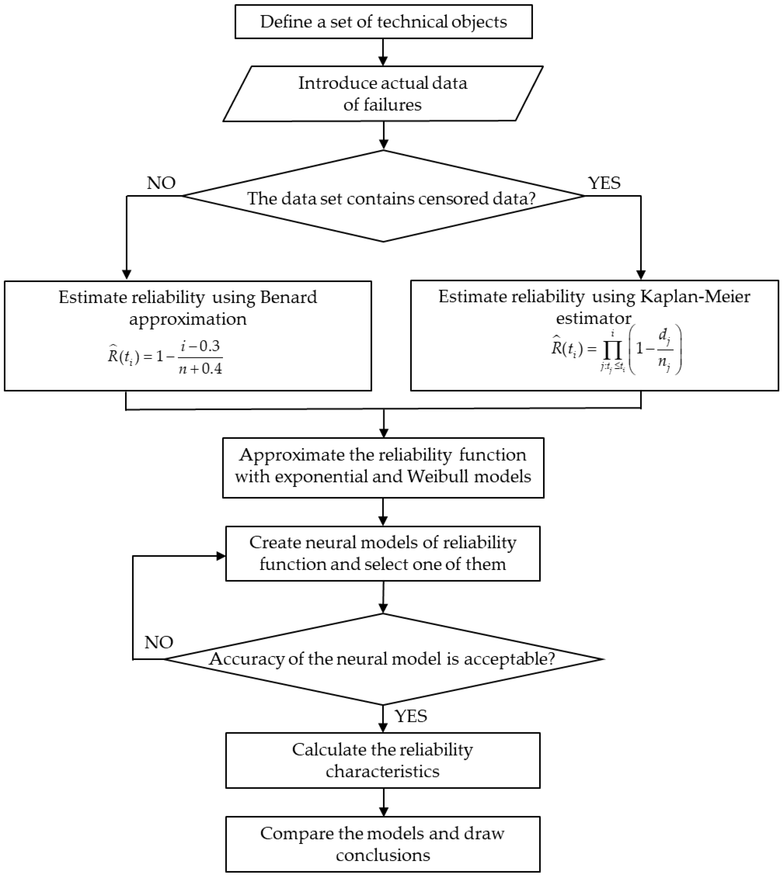
Figure 1 shows the author’s algorithm for analysing and modelling the reliability of technical objects. According to the given assumptions, the reliability study of technical objects begins with the identification of a representative group of objects working under indistinguishable operating conditions and performing the same work. The starting point for modelling reliability characteristics is the estimation of the value of the reliability function using empirical data. This is followed by an approximation of the reliability function using analytical and neural models. On the basis of the created reliability function models, the remaining characteristics are created, i.e., the failure probability density function and the failure intensity function.

Figure 1. Flowchart of reliability modelling.

2.1. Reliability Estimation

During the operation of technical facilities, the failure records form the basis for the development of reliability models. From this perspective, indices defining intervals to failure or between failure are useful [11,37]. These intervals can be expressed in operational units referring to the operating time of the object (h, mth) or to the mileage [km] in the case of vehicles. The following reliability indicators are identified [38,39,40,41]:

• Time to failure (TTF),
• Time between failures (TBF),
• Mileage to failure (MTF),
• Mileage between failures (MBF).

Based on a statistically significant sample of technical objects, an empirical reliability function is determined. The following equation can be used to determine it [35]:

$$\widehat{R}(t_i)=1-\frac{i}{n},$$

(5)

where t_i is the time of occurrence of the i-th failure, i is the number of failed technical objects up to time T_i, and n is the number of all technical objects belonging to the study sample.

However, this form of the empirical reliability function may cause distortion for values of i close to 0 and n. The solution to this problem is the Benard approximation commonly used in the literature [17,18,19,42], the form of which is shown in the equation:

$$\widehat{R}(t_i)=1-\frac{i-0.3}{n+0.4}.$$

(6)

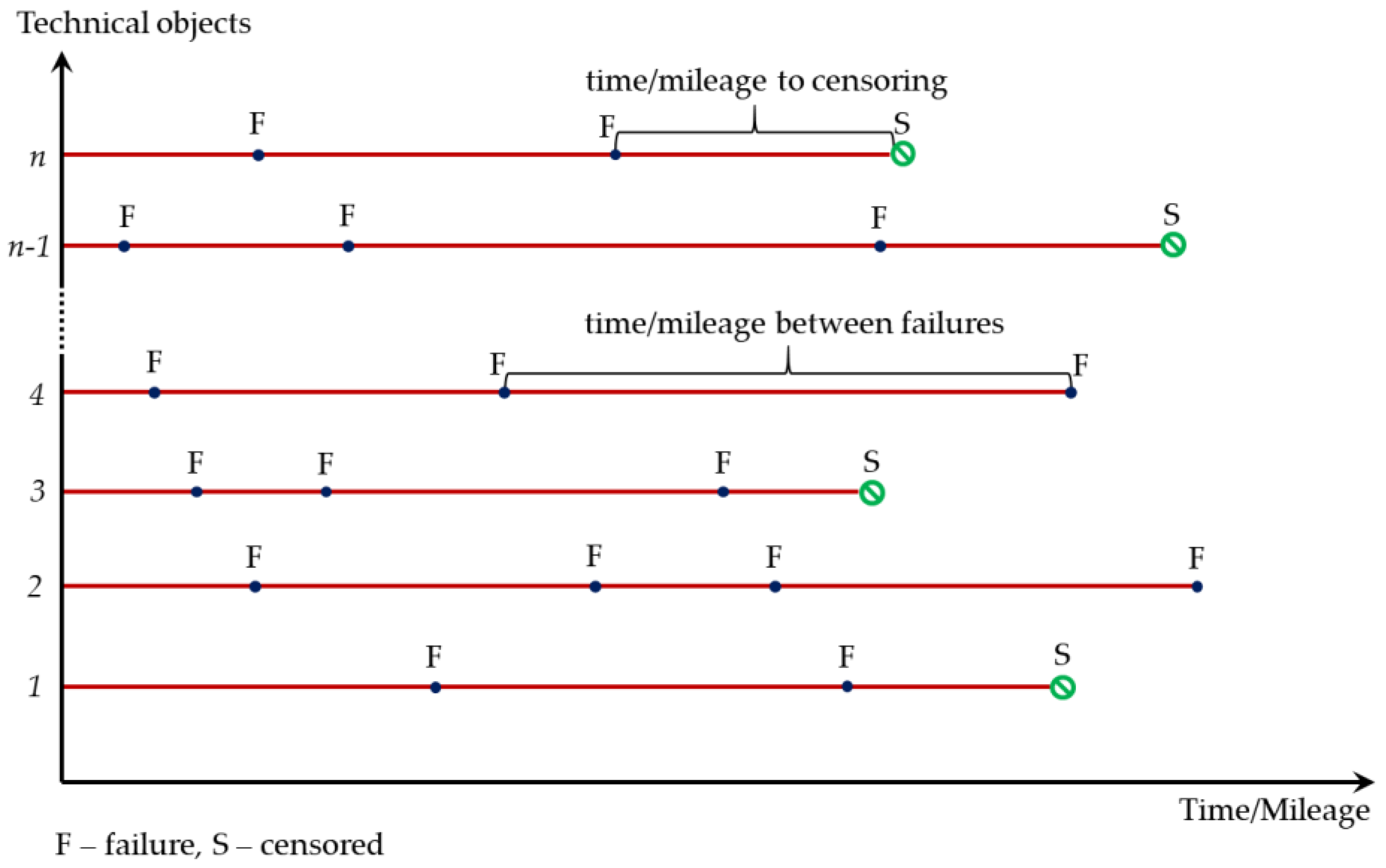
The above estimators are applicable to scientific studies of a specified sample of technical objects, assuming equal intensity of use of all objects and complete knowledge of the exploitation process. In real technical systems, including transport systems involving military vehicles, there are significant differences in the mileage achieved, despite the aim of even usage. It is therefore proposed to adopt the Kaplan–Meier estimator used in survival analysis to estimate the value of the reliability function. It allows the analysis of censored data, useful for studying certain periods of the exploitation process, in which, after having performed a certain amount of work expressed in exploitation units, did not suffer from failure until now or ceased to operate in a given system [14]. Figure 2 shows a graphical interpretation of the study period of the exploitation process, taking into account the censored data. The Kaplan–Meier estimator for the reliability function [14,43] is presented in the following equation:

$$\widehat{R}(t_i)={\displaystyle \prod _{j:t_j\le t_i}^i\left(1-\frac{d_j}{n_j}\right)},$$

(7)

where d_j is the number of technical objects that have sustained failure at time t_j, and n_j is the number of all technical objects that have lasted until time t_j.

Figure 2. Schematic of exploitation process with censored data.

The standard error [44,45] has been obtained by the Greenwood Formula (8):

$$SE\left\{\widehat{R}\left(t_i\right)\right\}=\widehat{R}\left(t_i\right)\sqrt{{\displaystyle \sum _{j=1}^i\frac{d_j}{n_j(n_j-d_j)}}}.$$

(8)

2.2. Exponential Model

The exponential model is a single-parameter distribution, described by the failure intensity λ, assuming λ = λ(t) = const. This model is applicable when describing the reliability of technical objects with a constant intensity of failure, which occurs as a result of random causes and not as a result of changes in technical conditions during the operation process. The reliability function for the exponential model takes the form:

$$R(t)=e^{-\lambda t}.$$

(9)

The failure probability density function for the exponential model takes the form:

$$f(t)=\lambda e^{-\lambda t}.$$

(10)

2.3. Weibull Model

The Weibull model is a two-parameter distribution used to describe the reliability of a technical object for which the failure intensity is time-varying. The reliability function in the Weibull model [42,46] is expressed by the relation:

$$R(t)=e^{-\beta t^{\alpha }}.$$

(11)

where α is the shape factor and β is the scale factor of the distribution.

After calculating the derivative from the failure function, a relation representing the failure probability density function is obtained:

$$f(t)=\alpha \beta t^{\alpha -1}{e}^{-\beta t^{\alpha }}.$$

(12)

After substituting the characteristics determined for the Weibull model into Equation (4), the failure intensity [47] can be expressed by the following equation:

$$\lambda (t)=\alpha \beta t^{\alpha -1}.$$

(13)

The parameter α determines the course of the failure intensity function of the technical object. For 0 < α < 1.0 the failure intensity function is decreasing, for α > 1.0 it is increasing, while for α = 1.0 it is constant and the distribution has the character of an exponential distribution.

2.4. Neural Modelling

Artificial neural networks are an advanced tool for modelling, classification and prediction of processes, phenomena and objects based on a set of data [48]. Multilayer Perceptron (MLP) is a neural network based on three types of neuron layers: input, hidden (or several hidden) and output [27,49,50]. The input layer neurons are responsible for sending input signals to the hidden layer neurons. For predictive models, the input signals are the normalised values of the explanatory variables. Hidden neurons aggregate the received input signals multiplied by the weights of the synaptic connections. The aggregated signal is the argument of the activation function, whose value is passed to the neurons of the next hidden layer or to the neurons of the output layer. The output layer neurons perform the same actions as the hidden neurons, except that the value obtained is equated to the value of the explanatory variable in the model [51,52,53].

The use of a simple neural network to approximate functions on the basis of estimated values obtained from empirical studies makes it possible to develop models that fit real data with a very high accuracy. Additionally, a regression network with an uncomplicated structure allows the approximating function to be written in analytical form.

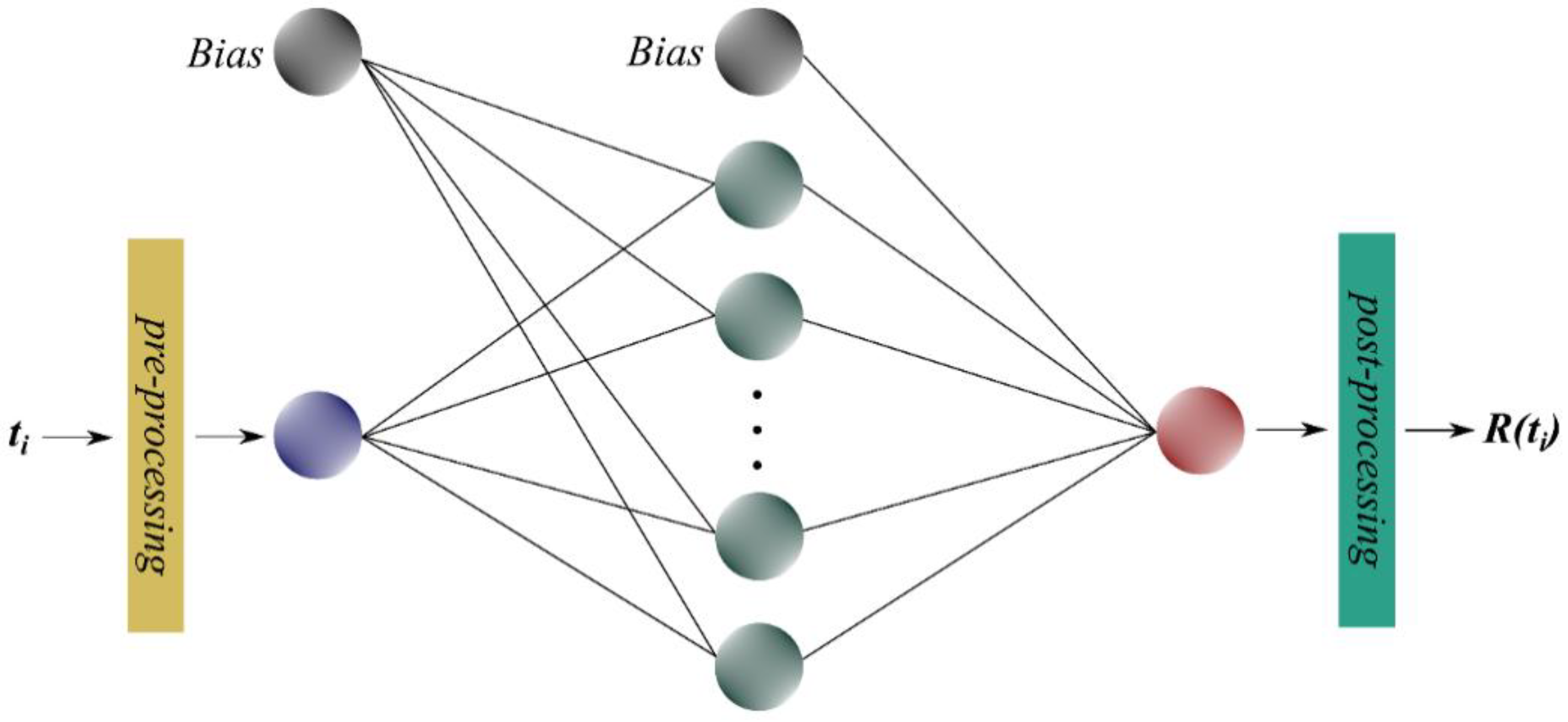
Figure 3 shows a flowchart illustrating the operation of the proposed neural network used to approximate the reliability function. The input signal is the mileage between failures, for which the value of the reliability function has been estimated. The output signal is the value of the reliability function. In the proposed neural model, the activation function of the hidden layer is a hyperbolic tangent, which ensures a fast learning process of the neural network [54,55]. For the output layer, on the other hand, activation occurs using a linear function.

Figure 3. Graph of neural network for reliability modelling.

If the variables x and y represent the normalised values of the variables t and R(t) according to the following relations:

$$x=\frac{2\left(t-t_{\min }\right)}{t_{\max }-t_{\min }}-1,$$

(14)

$$y=\frac{2\left(\widehat{R}(t)-\widehat{R}{(t)}_{\min }\right)}{\widehat{R}{(t)}_{\max }-\widehat{R}{(t)}_{\min }}-1.$$

(15)

Then the analytical form of the neural model is represented by the relation:

$$y=\left[{\displaystyle \sum _{n=1}^h\left(\left(\frac{2}{1+e^{-2\left(x{w}_{1n}+w_{0n}\right)}}-1\right)\cdot v_{n1}\right)}\right]+v_{01},$$

(16)

where h is the number of hidden neurons, w represents weights of synaptic connections between the input layer and the hidden layer, and v are weights of synaptic connections between the hidden layer and the output layer.

During the training process, the neural network, using the Levenberg–Marquardt algorithm, seeks to minimise the value of its error function, which is calculated according to the following formula:

$$E(n)=\frac{1}{2}{\displaystyle \sum _{i=1}^n{\left(\widehat{R}\left(t_i\right)-R_{out}\left(t_i\right)\right)}^2},$$

(17)

where $\widehat{R}(t_i)$ denotes the estimated value of the reliability function at point t_i, while $R_{out}(t_i)$ is the value obtained at the output of the neural network.

2.5. Accuracy of Fitting

An important part of carrying out reliability studies is assessing the accuracy of the developed models. In the literature, a number of measures and indicators are used to determine how accurately the model fits the empirical or estimated values. The authors of this publication used two indices in their reliability studies to completely assess the accuracy of the developed models in relation to the estimated values for a selected group of military vehicles. The first is the correlation coefficient R calculated according to the formula [56]:

$$R=\sqrt{1-\frac{{\displaystyle \sum _{i=1}^n{\left(\widehat{R}\left(t_i\right)-R_d\left(t_i\right)\right)}^2}}{{\displaystyle \sum _{i=1}^n{\left(\widehat{R}\left(t_i\right)-\frac{1}{n}\left({\displaystyle \sum _{i=1}^n\widehat{R}\left(t_i\right)}\right)\right)}^2}}},$$

(18)

where $\widehat{R}(t_i)$ is the estimated value of reliability function by Equation (7) and $R_d(t_i)$ is the fit value of the approximation model.

The second measure [56,57,58] is the Mean Squared Error (MSE) expressed per the formula:

$$MSE=\frac{1}{n}{\displaystyle \sum _{i=1}^n{\left(\widehat{R}(t_i)-R_d(t_i)\right)}^2}.$$

(19)

3. Results and Discussion

A selected sample of Honker military vehicles operated by a military unit of the Armed Forces of the Republic of Poland was used to carry out research on reliability characteristics. These are military vehicles with a maximum load capacity of approximately 1000.0 kg. Their tasks include transporting passengers and cargo on public roads as well as in off-road conditions.

Table 2 summarises the empirical data on mileages between failures. The data comes from the analysis of operational records and covers a 3-year study period in which 99 observations were recorded. The designation F refers to the mileage between failures, while S is the amount of mileage that the vehicle has completed until the end of the observation of a certain period of the service process without sustaining failure.

Table 2. Data set of mileages between failures of military vehicles.

No.	Mileage (km)	F/S	No.	Mileage (km)	F/S	No.	Mileage (km)	F/S	No.	Mileage (km)	F/S
1	18	S	26	949	F	51	2297	F	76	4418	S
2	36	F	27	993	F	52	2329	F	77	4472	F
3	38	S	28	1034	S	53	2546	F	78	4904	S
4	47	F	29	1066	S	54	2592	S	79	5177	S
5	59	F	30	1158	F	55	2666	F	80	5195	F
6	76	F	31	1159	S	56	2720	F	81	5387	S
7	80	S	32	1186	F	57	2792	F	82	5579	F
8	99	F	33	1224	F	58	2829	S	83	5664	S
9	112	F	34	1324	F	59	3002	F	84	5894	F
10	117	F	35	1352	F	60	3004	F	85	6103	F
11	148	S	36	1367	S	61	3087	F	86	6526	S
12	149	F	37	1390	F	62	3259	S	87	7442	F
13	264	F	38	1410	F	63	3386	F	88	7811	F
14	264	F	39	1523	F	64	3438	F	89	8252	S
15	273	S	40	1527	S	65	3457	S	90	8663	F
16	351	S	41	1588	F	66	3471	F	91	8761	F
17	361	F	42	1601	F	67	3515	S	92	9086	F
18	380	F	43	1639	F	68	3520	F	93	9653	S
19	438	F	44	1702	F	69	3600	F	94	10,459	F
20	494	F	45	1774	F	70	3605	F	95	11,072	F
21	631	F	46	1801	F	71	3717	F	96	11,404	S
22	690	F	47	2025	F	72	3780	F	97	12,618	F
23	708	F	48	2074	S	73	3874	F	98	14,977	S
24	790	F	49	2109	S	74	4202	F	99	21,477	S
25	949	F	50	2112	S	75	4244	F

3.1. Kaplan–Meier Estimation

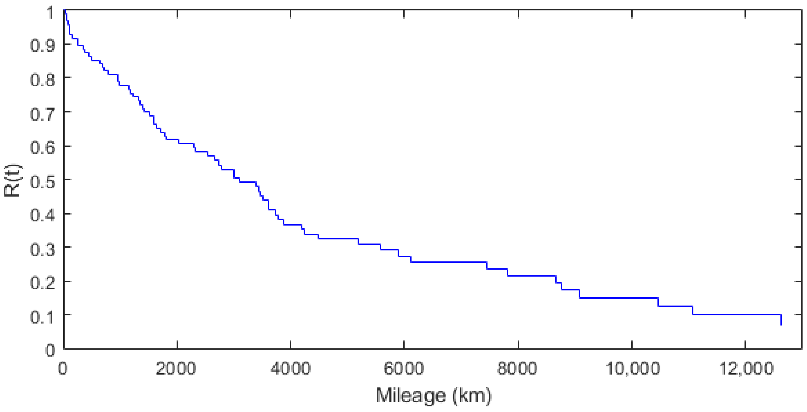
The Kaplan–Meier estimator was used to estimate the values of the unreliability and reliability functions. The study was based on the data in Table 2 and the relations (7) and (8). The results are presented in Table 3. The range of estimated values that will be used for approximation with reliability models includes the values of mileage at which the failure occurred and the initial value of 0.0. A graphical interpretation of the estimated values of the reliability function is presented using a staircase diagram in Figure 4.

Table 3. Estimated values of unreliability and reliability functions.

Mileage (km)	F(t)	R(t)	SE{R(t)}	Mileage (km)	F(t)	R(t)	SE{R(t)}
0	0.0000	1.0000	0.0000	2025	0.3948	0.6052	0.0512
36	0.0102	0.9898	0.0102	2297	0.4071	0.5929	0.0515
47	0.0205	0.9795	0.0144	2329	0.4195	0.5805	0.0519
59	0.0308	0.9692	0.0175	2546	0.4318	0.5682	0.0523
76	0.0411	0.9589	0.0201	2666	0.4444	0.5556	0.0526
99	0.0516	0.9484	0.0225	2720	0.4571	0.5429	0.0530
112	0.0620	0.9380	0.0245	2792	0.4697	0.5303	0.0532
117	0.0724	0.9276	0.0264	3002	0.4826	0.5174	0.0535
149	0.0829	0.9171	0.0281	3004	0.4956	0.5044	0.0537
264	0.1040	0.8960	0.0297	3087	0.5085	0.4915	0.0539
361	0.1148	0.8852	0.0311	3386	0.5218	0.4782	0.0541
380	0.1256	0.8744	0.0326	3438	0.5351	0.4649	0.0542
438	0.1364	0.8636	0.0339	3471	0.5487	0.4513	0.0543
494	0.1472	0.8528	0.0352	3520	0.5628	0.4372	0.0544
631	0.1580	0.8420	0.0364	3600	0.5769	0.4231	0.0545
690	0.1688	0.8312	0.0375	3605	0.5910	0.4090	0.0545
708	0.1796	0.8204	0.0385	3717	0.6051	0.3949	0.0545
790	0.1904	0.8096	0.0395	3780	0.6192	0.3808	0.0544
949	0.2120	0.7880	0.0404	3874	0.6333	0.3667	0.0543
993	0.2228	0.7772	0.0413	4202	0.6474	0.3526	0.0541
1158	0.2339	0.7661	0.0421	4244	0.6615	0.3385	0.0538
1186	0.2451	0.7549	0.0429	4472	0.6763	0.3237	0.0535
1224	0.2564	0.7436	0.0437	5195	0.6925	0.3075	0.0531
1324	0.2677	0.7323	0.0445	5579	0.7095	0.2905	0.0529
1352	0.2789	0.7211	0.0452	5894	0.7277	0.2723	0.0526
1390	0.2904	0.7096	0.0459	6103	0.7458	0.2542	0.0524
1410	0.3018	0.6982	0.0466	7442	0.7654	0.2346	0.0519
1523	0.3133	0.6867	0.0472	7811	0.7849	0.2151	0.0515
1588	0.3249	0.6751	0.0478	8663	0.8065	0.1935	0.0508
1601	0.3366	0.6634	0.0484	8761	0.8280	0.1720	0.0500
1639	0.3482	0.6518	0.0490	9086	0.8495	0.1505	0.0489
1702	0.3598	0.6402	0.0495	10,459	0.8746	0.1254	0.0473
1774	0.3715	0.6285	0.0500	11,072	0.8996	0.1004	0.0456
1801	0.3831	0.6169	0.0504	12,618	0.9331	0.0669	0.0428

Figure 4. Kaplan–Meier reliability estimation graph.

3.2. Exponential Model of Reliability

An approximation using Matlab software was used to determine the reliability function of military vehicles as a function of the mileage between failures. The parameter determination λ for the exponential model was done using the nonlinear least-squares method. The objective function is to minimise the sum of squares of the differences between the true values and the values achieved by the approximating function, according to the following equation [59,60,61]:

$$S_n(\lambda )={\displaystyle \sum _{i=1}^n{\left(\widehat{R}\left(t_i\right)-f\left(t_i,\lambda \right)\right)}^2},$$

(20)

where f(t_i,λ) is the value of the exponential reliability function R(t) with parameter λ for the value of t_i.

S_n(λ) takes the minimum value for the critical point, for which the following expression exists:

$$\frac{\partial S_n(\lambda )}{\partial \lambda }=0.$$

(21)

After transformations according to the chain rule, the above relation can be written by the equation:

$${\displaystyle \sum _{i=1}^n\left[\widehat{R}\left(t_i\right)-f\left(t_i,\lambda \right)\right]}\left(-\frac{\partial f\left(t_i,\lambda \right)}{\partial \lambda }\right)=0.$$

(22)

Model fitting was performed using the Trust Region algorithm [62,63] in the Curve Fitting Tool application (Matlab). The models were matched to the estimated values of functions presented in Table 3. The exponential model for approximating the reliability function of the studied sample of technical objects is presented in Equation (26):

$$R(t)=e^{-0.000235t}.$$

(23)

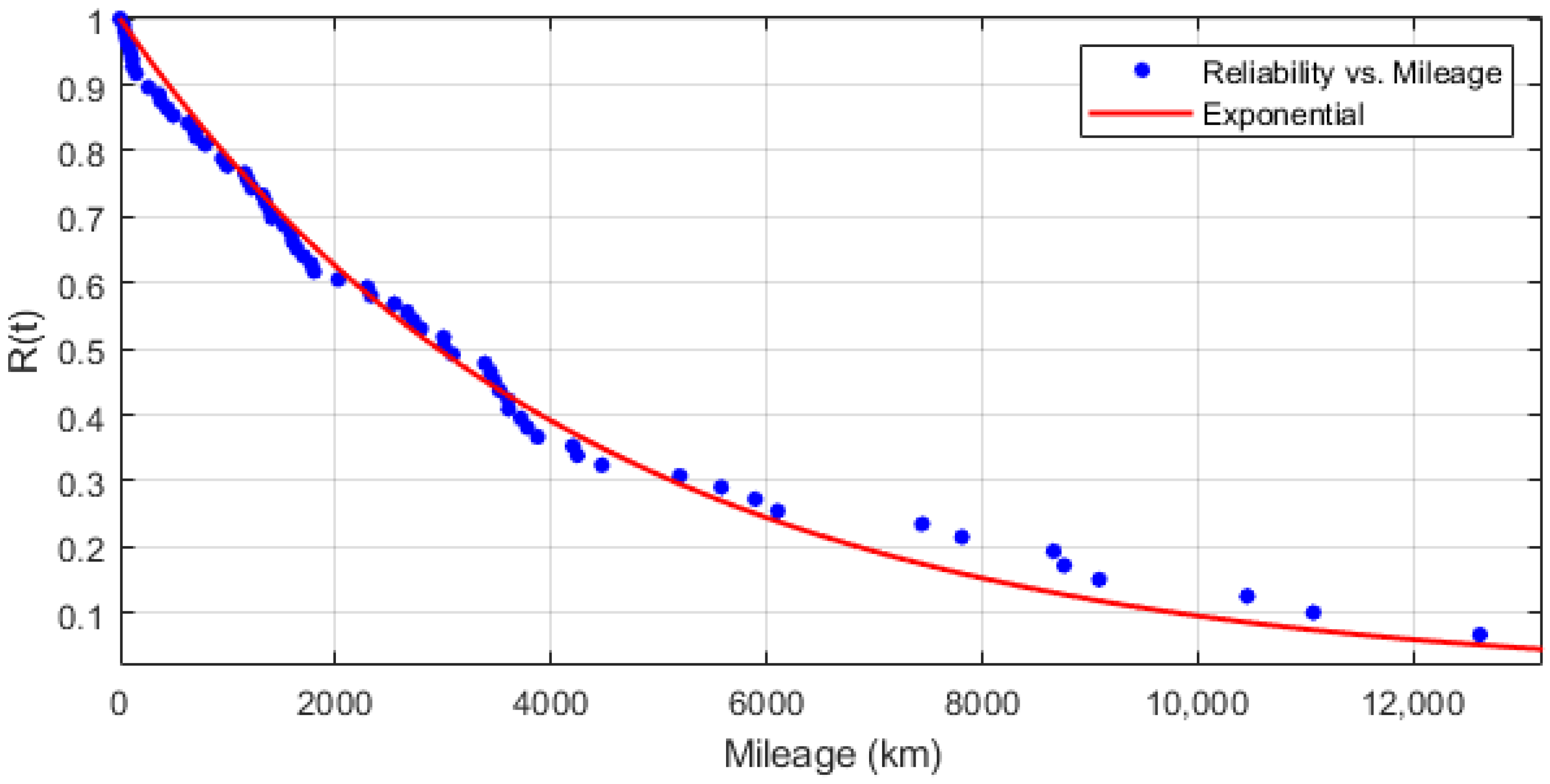
Figure 5 shows a graphical interpretation of how the exponential model fits the estimated values of the reliability function.

Figure 5. Graph presenting exponential model fitting to estimated values of reliability function.

3.3. Weibull Model of Reliability

The approximation of the reliability function R(t) with the Weibull model was performed using the nonlinear least-squares method, analogous to the exponential model. Selection of optimal values of parameters α and β was carried out with minimisation of the objective function according to the relation [59,60,61]:

$$S_n(\alpha ,\beta )={\displaystyle \sum _{i=1}^n{\left(\widehat{R}\left(t_i\right)-f\left(t_i,\alpha ,\beta \right)\right)}^2},$$

(24)

where f(t_i,α,β) is the value of the Weibull model of the reliability function R(t) with parameters α and β for the value of t_i.

S_n(α,β) takes the minimum value for the critical point for which the following relations are valid:

$$\frac{\partial S_n(\alpha ,\beta )}{\partial \alpha }=0,$$

(25)

$$\frac{\partial S_n(\alpha ,\beta )}{\partial \beta }=0.$$

(26)

Transforming the above relations, analogous to the case of the exponential model, the following two conditions are obtained:

$${\displaystyle \sum _{i=1}^n\left[\widehat{R}\left(t_i\right)-f\left(t_i,\alpha ,\beta \right)\right]}\left(-\frac{\partial f\left(t_i,\alpha ,\beta \right)}{\partial \alpha }\right)=0,$$

(27)

$${\displaystyle \sum _{i=1}^n\left[\widehat{R}\left(t_i\right)-f\left(t_i,\alpha ,\beta \right)\right]}\left(-\frac{\partial f\left(t_i,\alpha ,\beta \right)}{\partial \beta }\right)=0.$$

(28)

After the approximation by the nonlinear least-squares method, using the Trust Region algorithm [62,63], the two-parameter Weibull model was obtained, which is represented by the formula:

$$R(t)=e^{-0.000574t^{0.889}}.$$

(29)

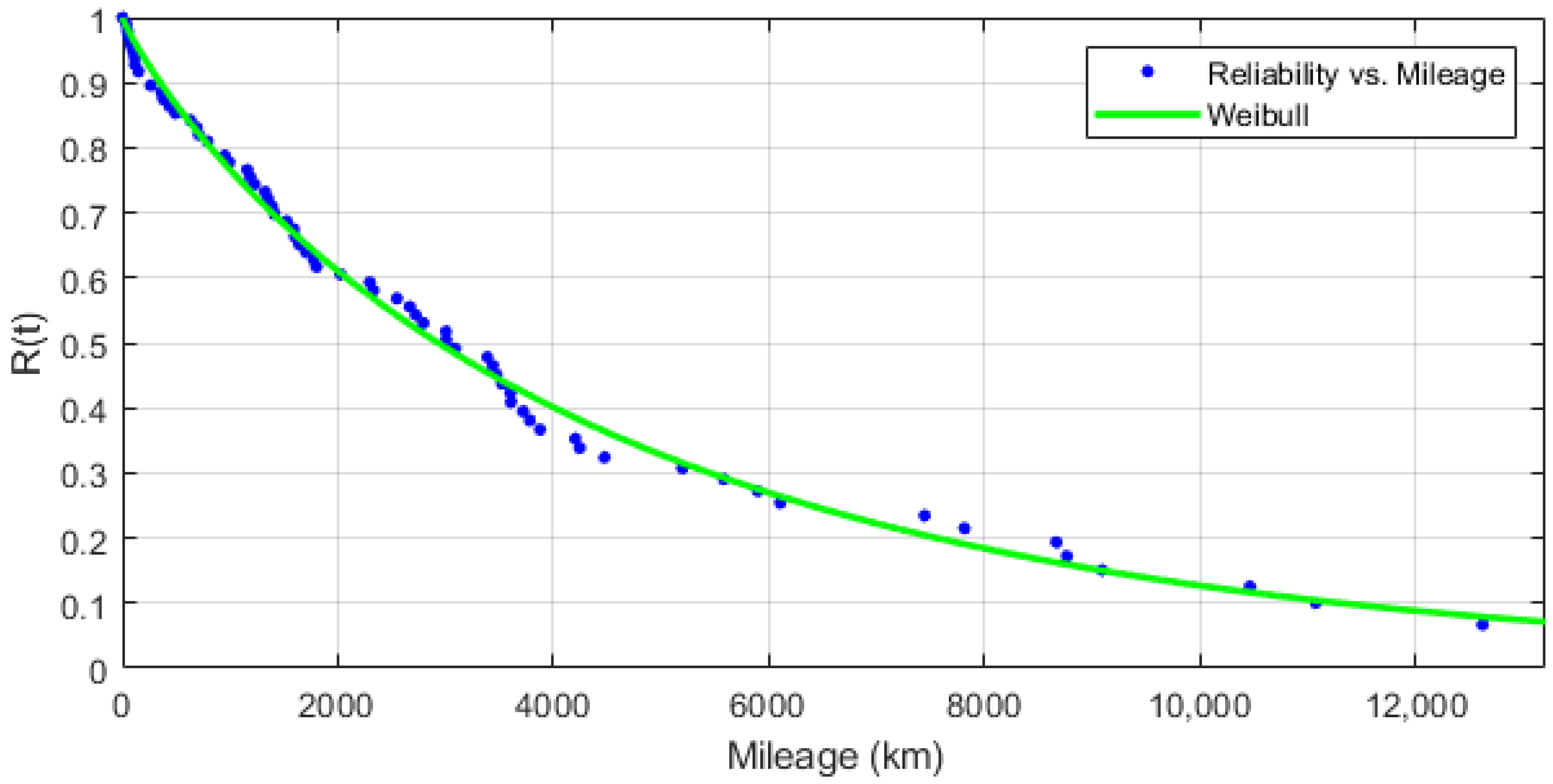
Figure 6 shows the course of the approximation curve with the points corresponding to the values obtained from the estimation. The small distances between the curve and the points indicate a good fit of the Weibull model.

Figure 6. Graph presenting Weibull model fitting to estimated values of reliability function.

3.4. Neural Model of Reliability

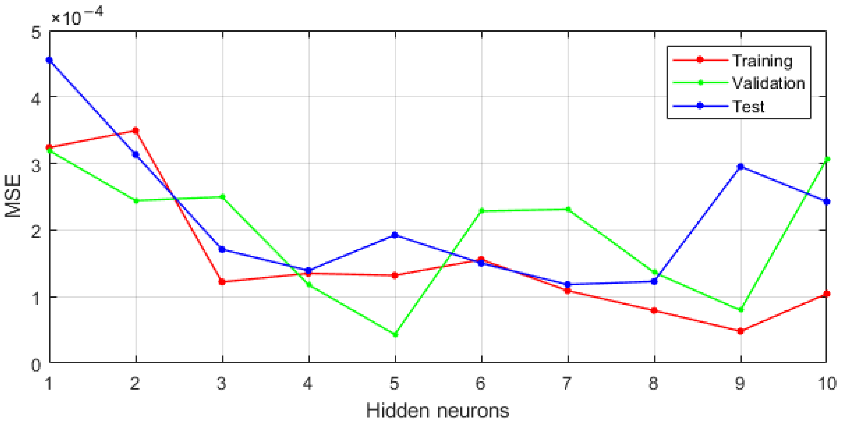
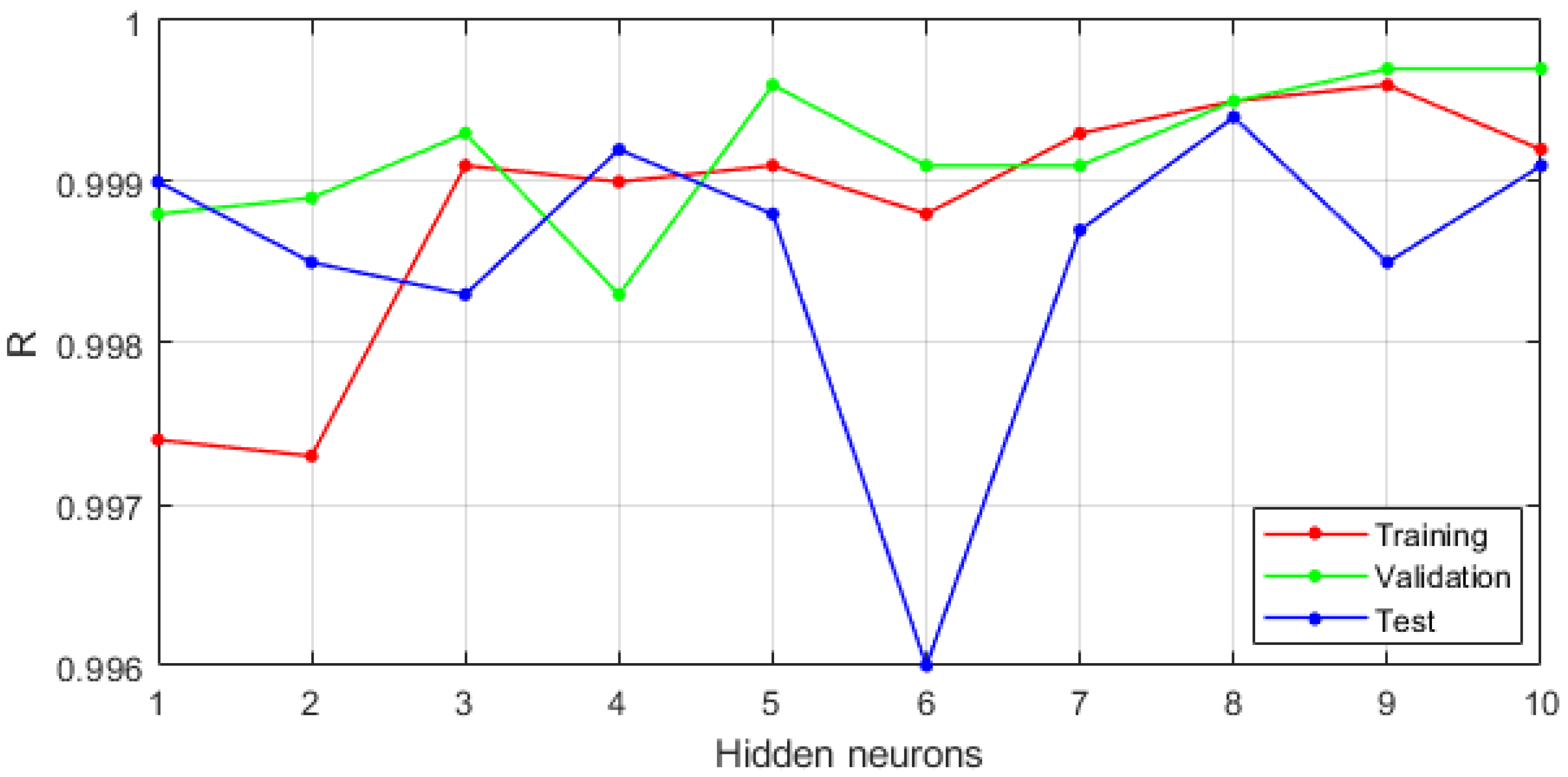
Neural modelling was carried out using IT support in the form of the Neural Net Fitting application in Matlab. The database was divided into three sets: training (80%), validation (10%) and test (10%). As part of the research conducted, 10 neural networks were created with varying numbers of neurons in the hidden layer. The results of model fitting are shown in Table 4 and in Figure 7 and Figure 8. Each of the trained neural networks showed very high prediction accuracy.

Table 4. R values of artificial neural networks.

MLP	Hidden Neurons	Training	Validation	Test
1-1-1	1	0.9974	0.9988	0.9990
1-2-1	2	0.9973	0.9989	0.9985
1-3-1	3	0.9991	0.9993	0.9983
1-4-1	4	0.9990	0.9983	0.9992
1-5-1	5	0.9991	0.9996	0.9988
1-6-1	6	0.9988	0.9991	0.9960
1-7-1	7	0.9993	0.9991	0.9987
1-8-1	8	0.9995	0.9995	0.9994
1-9-1	9	0.9996	0.9997	0.9985
1-10-1	10	0.9992	0.9997	0.9991

Figure 7. Sensitivity analysis of MSE error of neural model as a function of hidden neurons number.

Figure 8. Analysis of sensitivity of R correlation coefficient in neural model as a function of hidden neurons number.

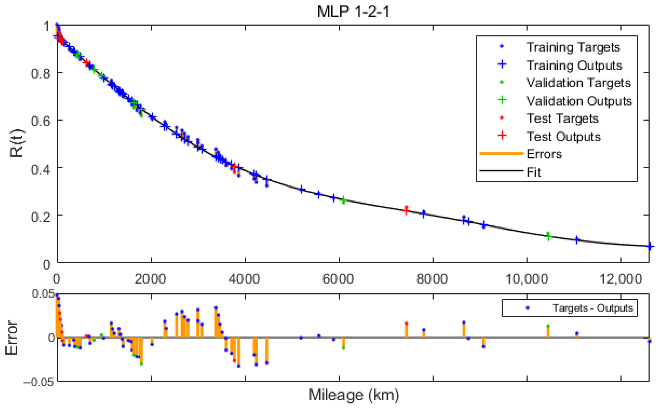
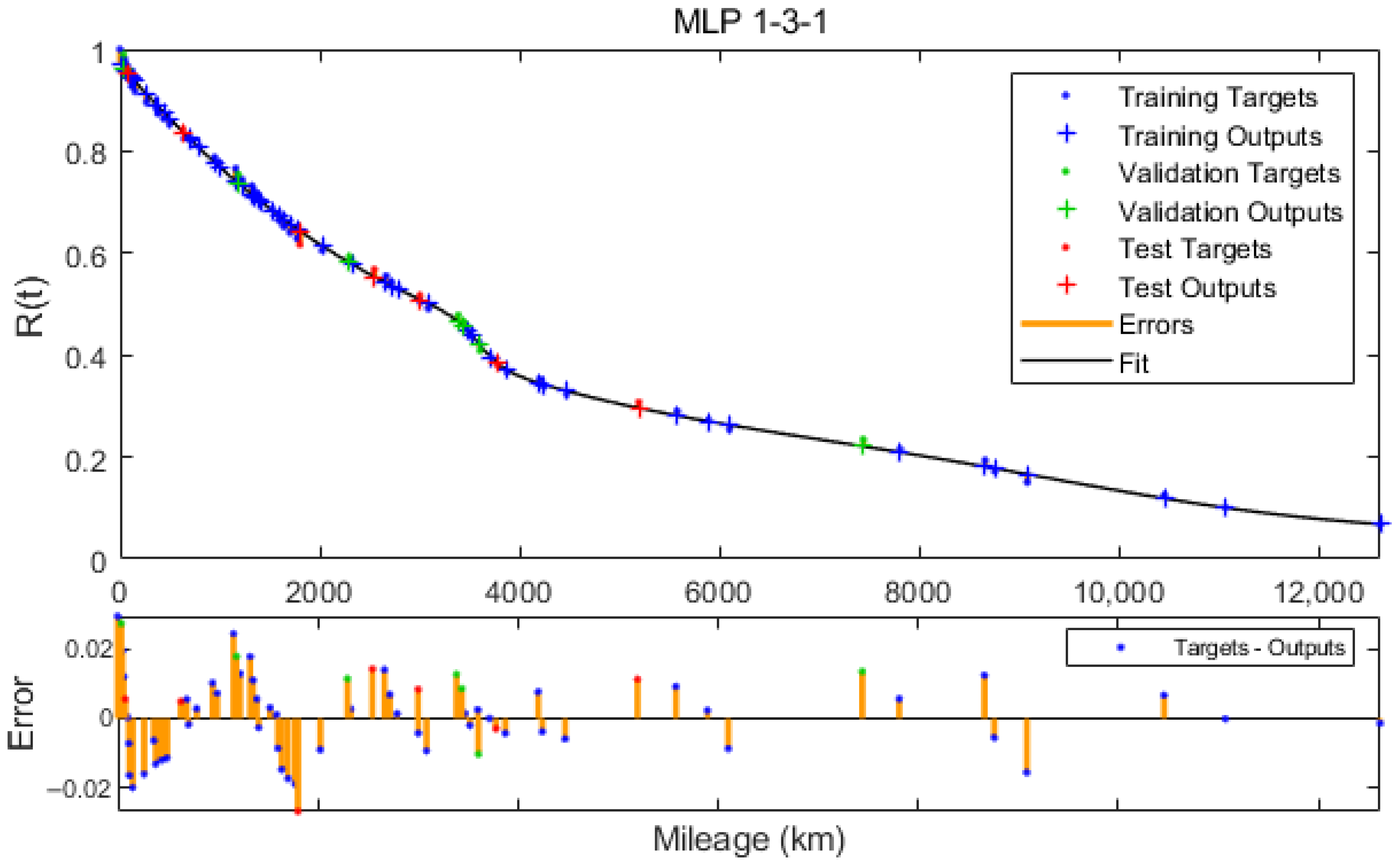
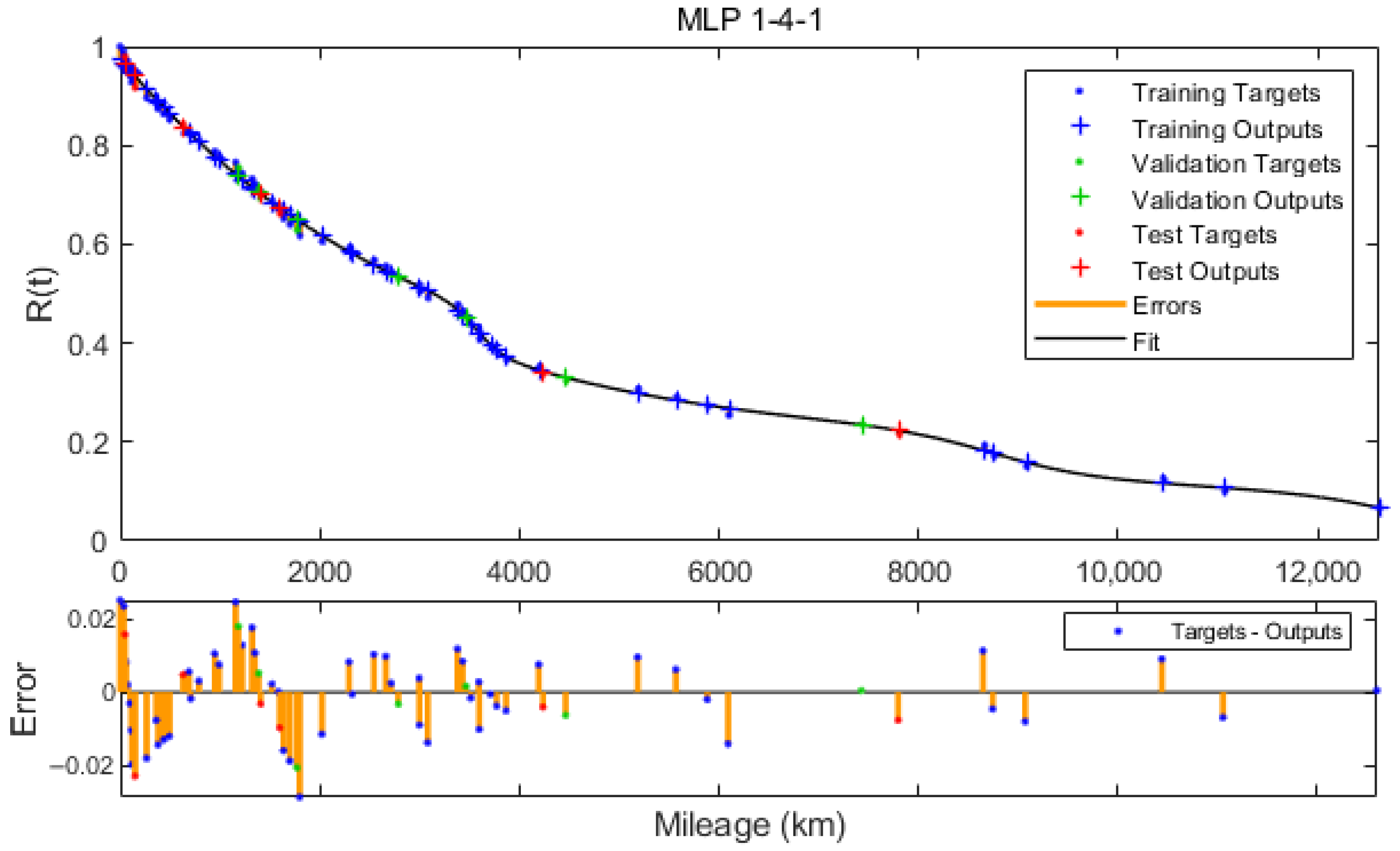
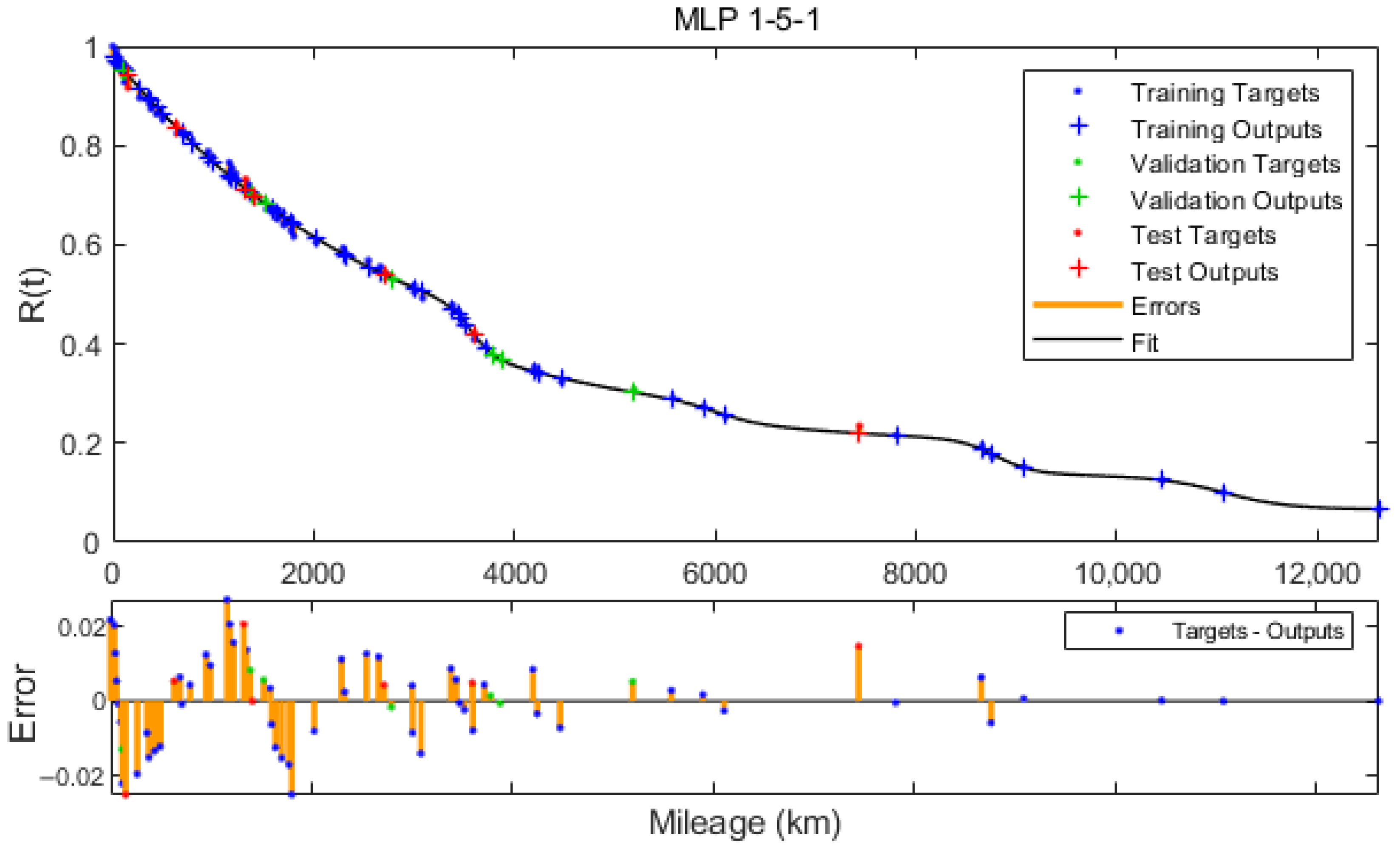
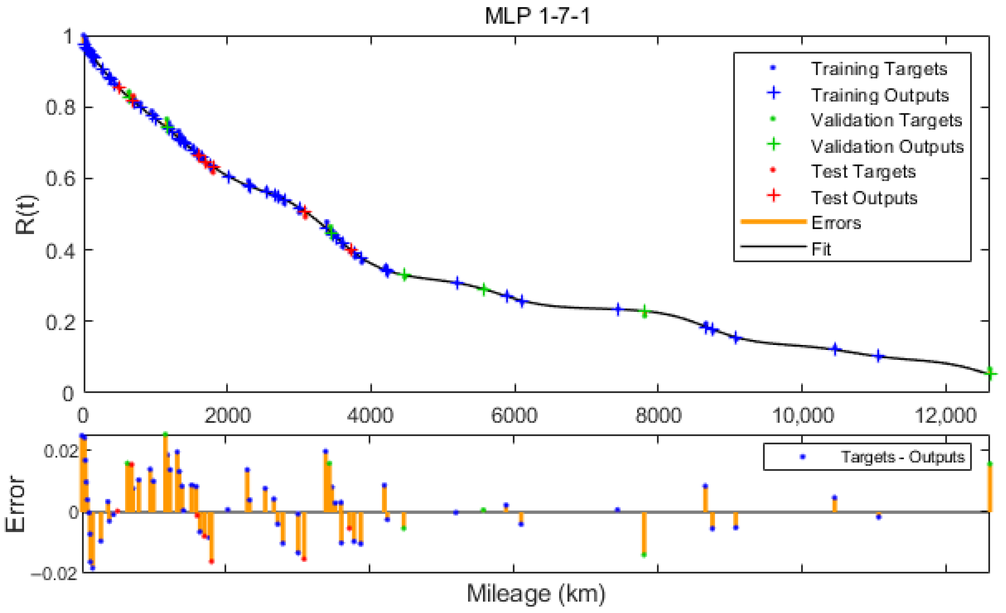
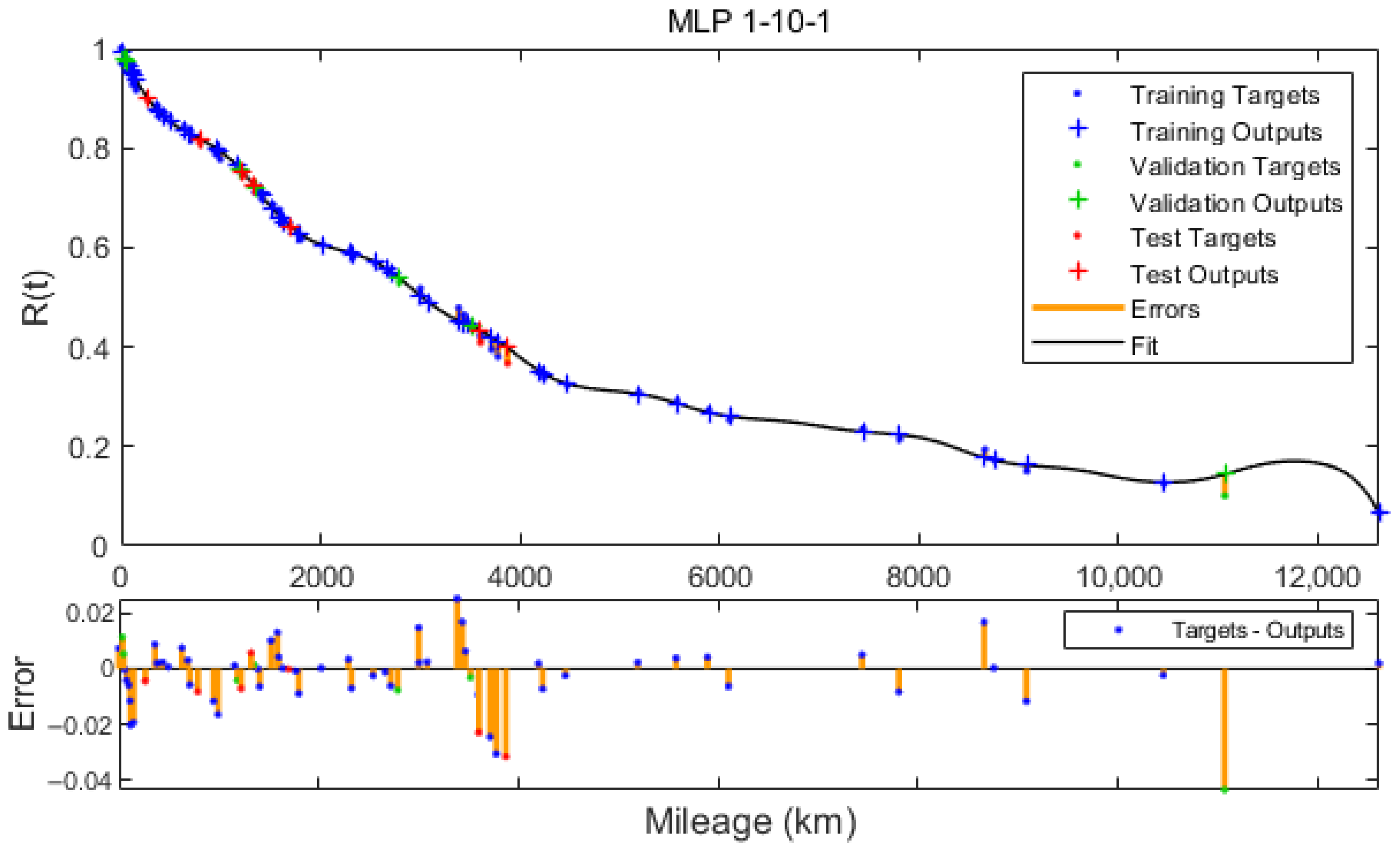
The analysis of the MSE error values and the R correlation coefficient presented in Figure 7 and Figure 8 show a slight improvement in the degree of fitting of the neural model to the estimated values of the reliability function. The graphs shown in Figure 9 and Figure A1, Figure A2, Figure A3, Figure A4, Figure A5, Figure A6, Figure A7, Figure A8 and Figure A9 (Appendix A) illustrate the approximation of the reliability function by neural models with a number of neurons in the hidden layer ranging from 1 to 10. While the number of hidden neurons increases, the model tends to interpolate the function. For a developed model based on 9 and 10 neurons, the approximating function takes a non-monotonic form and therefore does not satisfy the condition of non-increasing reliability function. The uncomplicated form and good fit of the MLP 1-1-1 model led us to choose this neural network as the suitable one for further analyses and considerations.

Figure 9. Reliability function approximated by MLP 1-1-1.

Figure 9 shows the course of the reliability function approximation curve in the MLP 1-1-1 neural model together with the estimated values and the difference between the estimated value and the modelled value. The degree of fitting in each dataset together with scatter plots are shown in Figure 10. The similar values of the R correlation coefficient indicate a valid approximation, without the occurrence of network overtraining and fitting only to the data from the training set.

Figure 10. MLP 1-1-1 regression plot.

The low complexity of the MLP 1-1-1 neural model makes it easy to obtain its analytical form. For the analysed example, the MLP 1-1-1 model can be represented by relation (29):

$$R(t)=\frac{32.925260+1.786689e^{0.000249t}}{1+34.674828e^{0.000249t}}.$$

(30)

3.5. Analysis of Reliability Models

The reliability function models developed as a result of the study showed a high degree of match with the estimated values. Table 5 summarises the values of the linear correlation coefficient R and the MSE error to compare the neural model with the exponential and Weibull models commonly used in literature. For all three models, the R correlation coefficient reached a value exceeding 0.99. However, the best fitting model is the neural model. The MSE error made by the MLP 1-1-1 is more than 2 times smaller than for the exponential model and about 14% smaller than the Weibull model.

Table 5. Accuracy of models.

Model	R	MSE
Exponential	0.9945	7.32 × 10−4
Weibull	0.9971	3.92 × 10−4
Neural	0.9975	3.37 × 10−4

The use of exponential and linear activation functions in the neural model allows for the utilisation of the differentiability of the analytical form of the approximating reliability function to calculate the relationships describing the failure probability density f(t) and the failure intensity λ(t). For the exponential and Weibull models, these relationships were developed according to the equations available in the literature. Table 6 shows the function f(t), while Table 7 presents the failure intensity λ(t) for each reliability model.

Table 6. Probability density functions.

Model	Probability Density Function
Exponential	$f(t)=0.000235e^{-0.000235t}$
Weibull	$f(t)=0.000510t^{-0.111}\cdot e^{-0.000574t^{0.889}}$
Neural	$f(t)=\frac{0.000236e^{0.000249t}}{{\left(0.028839+e^{0.000249t}\right)}^2}$

Table 7. Failure intensity functions.

Model	Failure Intensity Function
Exponential	$\lambda (t)=0.000235$
Weibull	$\lambda (t)=0.000510t^{-0.111}$
Neural	$\lambda (t)=\frac{0.297572e^{0.000498t}+0.008621e^{0.000249t}}{1+65.246821e^{0.000747t}+1206.137388e^{0.000498t}+69.404797e^{0.000249t}}$

To compare the courses of the individual reliability characteristics, their graphical interpretations are shown in Figure 11 and Figure 12. The probability density function has a very similar course for all three models. The Weibull model for the mileage in the 0.0 ÷ 1000.0 km range is an exception, for which the function f(t) significantly deviates from the values achieved by the other models. For all models, the function f(t) is decreasing.

Figure 11. Probability density functions of reliability models.

Figure 12. Failure intensity functions of reliability models.

The failure intensity function, which is the quotient of the failure probability density value and the reliability value, takes different courses for each of the three reliability models developed. For the exponential model, according to the theoretical assumptions, the function is constant and takes the value 0.000235 [1/km] for the studied sample of vehicles. For the Weibull model, the course of the function λ(t) for arguments 0.0 ÷ 1000.0 km is similar to that of the function f(t). This is due to the reliability function taking values close to one for these arguments. The further course of the intensity function for the Weibull model is flattened and reaches values smaller than in the exponential model. In the neural model, the function λ(t) is decreasing, with values smaller than in the exponential model for the whole domain resulting from the model constraints.

Figure 13 presents a plot showing the value of the integral of the reliability function over the integration interval [0.0, t] for t ≤ 100,000.0 km. The calculated definite integral in the interval from 0.0 to infinity corresponds to the expected value of the mileage between failures. For the exponential and Weibull model, the expected value of ET is finite and is 4255.32 km and 4686.22 km, respectively (Table 8). For the neural model, the expected value of the mileage between failures approaches infinity. The use of the model, therefore, requires the implementation of appropriate constraints due to the inability of the neural network to extrapolate the value of the reliability function beyond the known data range. The empirical data for which the value of the reliability function was estimated range between [0.0; 21,477.0 km]. In this range, the ET value for the neural model attains similar levels to the Weibull model.

Figure 13. Definite integral graph of reliability function depending on integration interval.

Table 8. Expected mileage between failures.

Model	ET (km)
Exponential	4255.32
Weibull	4686.22
Neural	-

The value of the expected mileage between failures can be an indicator that determines the intervals between periodic inspections and maintenance of technical objects. Appropriate adjustment of the maintenance intervals according to the determined reliability characteristics can positively influence the readiness of the technical object and can increase the probability of a task being properly carried out without failure occurring.

4. Conclusions

In this publication, research has been carried out concerning the reliability modelling of military vehicles. A methodology based on the use of non-parametric estimation and reliability function approximation has been proposed. The estimation of the reliability function values was carried out using the Kaplan–Meier estimator. As opposed to the Benard approximation, it enables the study to be carried out on censored data. The estimated values of the reliability function were used to develop mathematical and neural models. From the set of developed neural models, based on the analysis of the MSE error values and the correlation coefficient R and taking into account the low complexity of the model form, the MLP 1-1-1 model was selected. Then, the analytical form of the neural model was created, which allowed its further analysis. After comparing the exponential, Weibull and MLP 1-1-1 models, the neural model proved to be the best match for the estimated reliability function values. This confirms the feasibility of using artificial neural networks for accurate function approximation.

Based on the approximated reliability functions, the reliability characteristics have been developed, i.e., the failure probability density functions, the failure intensity functions and the expected values of the mileage between failures. The plot of the failure probability density function was similar for all 3 models for mileage values exceeding 1000.0 km. The failure intensity function for the exponential model, according to the theoretical assumptions, is constant. For the Weibull and neural models, the course of the function λ(t) showed a decreasing monotonicity, but with different values.

The expected mileage between failures, calculated as the definite integral of the reliability function, took a finite value for the exponential and Weibull models, reaching 4255.32 km and 4686.22 km, respectively. For the neural model, the expected value approached infinity. The above fact indicates the inability of the neural network to extrapolate the reliability function. Thus, when using a neural model, it is necessary to impose constraints derived from the empirical data set. The practical aspect of determining the ET (expected mileage between failures) value can be to use it as an indicator for planning periodic vehicle maintenance. The purpose of periodic servicing is to restore the technical life and minimise the risk of failure and malfunction. The technical system, in which the analysed group of vehicles operates, assumes the realisation of preventive maintenance at intervals of 1 calendar year or every 5000.0 km of the mileage. Comparing this value to the expected mileage between failures, it can be concluded that the periodic services are carried out too rarely, which causes frequent failures and negatively affects the reliability of military vehicles.

So far, the applications of artificial neural networks for modelling the reliability of technical objects have been focused mainly on the precise predictions of reliability function values and the times of subsequent failure occurrences. This study goes beyond these areas of application, as the focus is on creating an accurate neural model that can be expressed in terms of analytical relationships. This approach allows further analysis of the model and determination of the remaining reliability characteristics.

The presented reliability testing methodology allows for the analysis and assessment of the reliability of military vehicles based on the observation of a certain period of operation in natural conditions, without the need for costly experiments and time-consuming simulations. This helps to avoid excessive costs associated with the implementation of experimental studies while ensuring the reliability of the analyses carried out.

References

- Li, X.; Zhao, X.; Pu, W. Knowledge-Oriented Modeling for Influencing Factors of Battle Damage in Military Industrial Logistics: An Integrated Method. Def. Technol. 2020, 16, 571–587. [Google Scholar] [CrossRef]
- Wróblewski, P.; Drożdż, W.; Lewicki, W.; Miązek, P. Methodology for Assessing the Impact of Aperiodic Phenomena on the Energy Balance of Propulsion Engines in Vehicle Electromobility Systems for Given Areas. Energies 2021, 14, 2314. [Google Scholar] [CrossRef]
- Barabino, B.; Di Francesco, M.; Mozzoni, S. An Offline Framework for the Diagnosis of Time Reliability by Automatic Vehicle Location Data. IEEE Trans. Intell. Transp. Syst. 2017, 18, 583–594. [Google Scholar] [CrossRef]
- Barabino, B.; Di Francesco, M.; Mozzoni, S. Time Reliability Measures in Bus Transport Services from the Accurate Use of Automatic Vehicle Location Raw Data. Qual. Reliab. Eng. Int. 2017, 33, 969–978. [Google Scholar] [CrossRef]
- Ziółkowski, J.; Małachowski, J.; Oszczypała, M.; Szkutnik-Rogoż, J.; Lęgas, A. Modelling of the Military Helicopter Operation Process in Terms of Readiness. Def. Sci. J. 2021, 71, 602–611. [Google Scholar] [CrossRef]
- Simiński, P.; Kończak, J.; Przybysz, K. Analysis and Testing of Reliability of Military Vehicles. J. KONBiN 2018, 47, 87–95. [Google Scholar] [CrossRef]
- Dobrzinskij, N.; Fedaravicius, A.; Pilkauskas, K.; Slizys, E. Impact of Climatic Conditions on the Parameters of Failure Flow of Military Vehicles. Proc. Inst. Mech. Eng. Part D J. Automob. Eng. 2021, 236, 753–762. [Google Scholar] [CrossRef]
- Żurek, J.; Zieja, M.; Ziółkowski, J.; Borucka, A. Vehicle Operation Process Analysis Using the Markov Processes. In Proceedings of the 29th European Safety and Reliability Conference (ESREL), Hannover, Germany, 22–26 September 2019; pp. 2598–2605. [Google Scholar]
- Li, Z.; Hensher, D.A.; Rose, J.M. Willingness to Pay for Travel Time Reliability in Passenger Transport: A Review and Some New Empirical Evidence. Transp. Res. Part E Logist. Transp. Rev. 2010, 46, 384–403. [Google Scholar] [CrossRef]
- Żurek, J.; Zieja, M.; Ziółkowski, J. Reliability of Supplies in a Manufacturing Enterprise. In Safety and Reliability–Safe Societies in a Changing World; CRC Press: Boca Raton, FL, USA, 2018; pp. 3143–3148. [Google Scholar]
- Jakkula, B.; Govinda, R.; Murthy, C.S.N. Maintenance Management of Load Haul Dumper Using Reliability Analysis. J. Qual. Maint. Eng. 2019, 26, 290–310. [Google Scholar] [CrossRef]
- Alkaff, A.; Qomarudin, M.N.; Purwantini, E.; Wiratno, S.E. Dynamic Reliability Modeling for General Standby Systems. Comput. Ind. Eng. 2021, 161, 107615. [Google Scholar] [CrossRef]
- Dziubak, T.; Wysocki, T.; Dziubak, S. Selection of Vehicles for Fleet of Transport Company on the Basis of Observation of Their Operational Reliability. Eksploat. I Niezawodn. Maint. Reliab. 2021, 23, 184–194. [Google Scholar] [CrossRef]
- Selech, J.; Andrzejczak, K. An Aggregate Criterion for Selecting a Distribution for Times to Failure of Components of Rail Vehicles. Maint. Reliab. 2019, 22, 102–111. [Google Scholar] [CrossRef]
- Woch, M.; Zieja, M.; Tomaszewska, J. Analysis of the Time between Failures of Aircrafts. In Proceedings of the 2017 2nd International Conference on System Reliability and Safety (ICSRS), Milan, Italy, 20–22 December 2017; pp. 112–118. [Google Scholar]
- Thijssens, O.W.M.; Verhagen, W.J.C. Application of Extended Cox Regression Model to Time-On-Wing Data of Aircraft Repairables. Reliab. Eng. Syst. Saf. 2020, 204, 107136. [Google Scholar] [CrossRef]
- Xu, K.; Xie, M.; Tang, L.C.; Ho, S.L. Application of Neural Networks in Forecasting Engine Systems Reliability. Appl. Soft Comput. 2003, 2, 255–268. [Google Scholar] [CrossRef]
- Chen, K.-Y. Forecasting Systems Reliability Based on Support Vector Regression with Genetic Algorithms. Reliab. Eng. Syst. Saf. 2007, 92, 423–432. [Google Scholar] [CrossRef]
- Da Chagas Moura, M.; Zio, E.; Lins, I.D.; Droguett, E. Failure and Reliability Prediction by Support Vector Machines Regression of Time Series Data. Reliab. Eng. Syst. Saf. 2011, 96, 1527–1534. [Google Scholar] [CrossRef]
- Chatterjee, S.; Bandopadhyay, S. Reliability Estimation Using a Genetic Algorithm-Based Artificial Neural Network: An Application to a Load-Haul-Dump Machine. Expert Syst. Appl. 2012, 39, 10943–10951. [Google Scholar] [CrossRef]
- Bai, B.; Zhang, J.; Wu, X.; Zhu, G.W.; Li, X. Reliability Prediction-Based Improved Dynamic Weight Particle Swarm Optimization and Back Propagation Neural Network in Engineering Systems. Expert Syst. Appl. 2021, 177, 114952. [Google Scholar] [CrossRef]
- Yan, W.X.; Pin, W.; He, L. Reliability Prediction of CNC Machine Tool Spindle Based on Optimized Cascade Feedforward Neural Network. IEEE Access 2021, 9, 60682–60688. [Google Scholar] [CrossRef]
- Du, Y.; Wu, G.; Tang, Y.; Liu, S. A Two-Stage Reliability Allocation Method for Remanufactured Machine Tools Integrating Neural Networks and Remanufacturing Coefficient. Comput. Ind. Eng. 2022, 163, 107834. [Google Scholar] [CrossRef]
- Liu, D.; Wang, S. An Artificial Neural Network Supported Stochastic Process for Degradation Modeling and Prediction. Reliab. Eng. Syst. Saf. 2021, 214, 107738. [Google Scholar] [CrossRef]
- Liu, D.; Wang, S.; Cui, X. An Artificial Neural Network Supported Wiener Process Based Reliability Estimation Method Considering Individual Difference and Measurement Error. Reliab. Eng. Syst. Saf. 2022, 218, 108162. [Google Scholar] [CrossRef]
- Kamruzzaman, M.; Bhusal, N.; Benidris, M. A Convolutional Neural Network-Based Approach to Composite Power System Reliability Evaluation. Int. J. Electr. Power Energy Syst. 2022, 135, 107468. [Google Scholar] [CrossRef]
- Lolas, S.; Olatunbosun, O.A. Prediction of Vehicle Reliability Performance Using Artificial Neural Networks. Expert Syst. Appl. 2008, 34, 2360–2369. [Google Scholar] [CrossRef]
- Lins, I.D.; das Chasgas Moura, M.; Zio, E.; Droguett, E.L. A Particle Swarm-Optimized Support Vector Machine for Reliability Prediction. Qual. Reliab. Eng. Int. 2012, 28, 141–158. [Google Scholar] [CrossRef]
- Krishna Mohan, G.; Yoshitha, N.; Lavanya, M.L.N.; Krishna Priya, A. Assessment and Analysis of Software Reliability Using Machine Learning Techniques. Int. J. Eng. Technol. (UAE) 2018, 7, 201–205. [Google Scholar] [CrossRef]
- Hraiba, A.; Touil, A.; Mousrij, A. Artificial Neural Network Based Hybrid Metaheuristics for Reliability Analysis. IFAC-Pap. 2020, 53, 654–660. [Google Scholar] [CrossRef]
- Hao, S.; Yang, J.; Ma, X.; Zhao, Y. Reliability Modeling for Mutually Dependent Competing Failure Processes Due to Degradation and Random Shocks. Appl. Math. Model. 2017, 51, 232–249. [Google Scholar] [CrossRef]
- Hong, L.; Zhai, Q.; Wang, X.; Ye, Z.-S. System Reliability Evaluation Under Dynamic Operating Conditions. IEEE Trans. Reliab. 2019, 68, 800–809. [Google Scholar] [CrossRef]
- Qi, S.; Huang, G.; Zhi, X.; Fan, F.; Flay, R.G.J. External Blast Load Factors for Dome Structures Based on Reliability. Def. Technol. 2021, 18, 170–182. [Google Scholar] [CrossRef]
- Dong, Y.; Lu, H.; Li, L. Reliability Sensitivity Analysis Based on Multi-Hyperplane Combination Method. Def. Technol. 2014, 10, 354–359. [Google Scholar] [CrossRef]
- Żurek, J.; Machałowski, J.; Ziółkowski, J.; Szkutnik-Rogoż, J. Reliability Analysis of Technical Means of Transport. Appl. Sci. 2020, 9, 3016. [Google Scholar] [CrossRef]
- Wu, B.; Cui, L. Reliability Evaluation of Markov Renewal Shock Models with Multiple Failure Mechanisms. Reliab. Eng. Syst. Saf. 2020, 202, 107051. [Google Scholar] [CrossRef]
- Tsarouhas, P. Reliability, Availability, and Maintainability (RAM) Study of an Ice Cream Industry. Appl. Sci. 2020, 10, 4265. [Google Scholar] [CrossRef]
- Stavropoulos, C.N.; Fassois, S.D. Non-Stationary Functional Series Modeling and Analysis of Hardware Reliability Series: A Comparative Study Using Rail Vehicle Interfailure Times. Reliab. Eng. Syst. Saf. 2000, 68, 169–183. [Google Scholar] [CrossRef]
- Wu, X.; Chang, Y.; Mao, J.; Du, Z. Predicting Reliability and Failures of Engine Systems by Single Multiplicative Neuron Model with Iterated Nonlinear Filters. Reliab. Eng. Syst. Saf. 2013, 119, 244–250. [Google Scholar] [CrossRef]
- Dai, Y.; Zhou, Y.; Jia, Y. Distribution of Time between Failures of Machining Center Based on Type I Censored Data. Reliab. Eng. Syst. Saf. 2003, 79, 377–379. [Google Scholar] [CrossRef]
- Petritoli, E.; Leccese, F.; Ciani, L. Reliability and Maintenance Analysis of Unmanned Aerial Vehicles. Sensors 2018, 18, 3171. [Google Scholar] [CrossRef]
- Rajpal, P.S.; Shishodia, K.S.; Sekhon, G.S. An Artificial Neural Network for Modeling Reliability, Availability and Maintainability of a Repairable System. Reliab. Eng. Syst. Saf. 2006, 91, 809–819. [Google Scholar] [CrossRef]
- Kaplan, E.L.; Meier, P. Nonparametric Estimation from Incomplete Observations. J. Am. Stat. Assoc. 1958, 53, 457–481. [Google Scholar] [CrossRef]
- Pokhrel, A.; Dyba, T.; Hakulinen, T. A Greenwood Formula for Standard Error of the Age-Standardised Relative Survival Ratio. Eur. J. Cancer 2008, 44, 441–447. [Google Scholar] [CrossRef]
- Cantor, A.B. Projecting the Standard Error of the Kaplan-Meier Estimator. Statist. Med. 2001, 20, 2091–2097. [Google Scholar] [CrossRef] [PubMed]
- Santhosh, T.V.; Gopika, V.; Ghosh, A.K.; Fernandes, B.G. An Approach for Reliability Prediction of Instrumentation & Control Cables by Artificial Neural Networks and Weibull Theory for Probabilistic Safety Assessment of NPPs. Reliab. Eng. Syst. Saf. 2018, 170, 31–44. [Google Scholar] [CrossRef]
- Wang, P.; Fan, J.; Li, Z. Study on Mean Time Between Failures Prediction Algorithms Based on Weibull Distribution. IOP Conf. Ser. Earth Environ. Sci. 2020, 440, 22083. [Google Scholar] [CrossRef]
- Li, Z.; Li, Z.; Li, Y.; Tao, J.; Mao, Q.; Zhang, X. An Intelligent Diagnosis Method for Machine Fault Based on Federated Learning. Appl. Sci. 2021, 11, 12117. [Google Scholar] [CrossRef]
- He, F.; Qi, H. A Method of Estimating Network Reliability Using an Artificial Neural Network. In Proceedings of the 2008 IEEE Pacific-Asia Workshop on Computational Intelligence and Industrial Application, Wuhan, China, 19–20 December 2008; Volume 2, pp. 57–60. [Google Scholar]
- Song, C.-Y. A Study on Learning Parameters in Application of Radial Basis Function Neural Network Model to Rotor Blade Design Approximation. Appl. Sci. 2021, 11, 6133. [Google Scholar] [CrossRef]
- Yang, R.; Zhang, L.; Cai, W.; Liu, Y.; Huang, H.-Z. Using Neural Network to Predict Reliability of Lithography Machine. In Proceedings of the 2013 International Conference on Quality, Reliability, Risk, Maintenance, and Safety Engineering (QR2MSE), Chengdu, China, 15–18 July 2013; pp. 308–311. [Google Scholar]
- Ziółkowski, J.; Oszczypała, M.; Małachowski, J.; Szkutnik-Rogoż, J. Use of Artificial Neural Networks to Predict Fuel Consumption on the Basis of Technical Parameters of Vehicles. Energies 2021, 14, 2639. [Google Scholar] [CrossRef]
- Aminisharifabad, M.; Yang, Q.; Wu, X. A Deep Learning-Based Reliability Model for Complex Survival Data. IEEE Trans. Reliab. 2021, 70, 73–81. [Google Scholar] [CrossRef]
- Izquierdo, J.; Crespo Márquez, A.; Uribetxebarria, J. Dynamic Artificial Neural Network-Based Reliability Considering Operational Context of Assets. Reliab. Eng. Syst. Saf. 2019, 188, 483–493. [Google Scholar] [CrossRef]
- Ching, T.; Zhu, X.; Garmire, L.X. Cox-Nnet: An Artificial Neural Network Method for Prognosis Prediction of High-Throughput Omics Data. PLoS Comput. Biol. 2018, 14, e1006076. [Google Scholar] [CrossRef]
- Li, X.-Y.; Tao, Z.; Wu, J.-P.; Zhang, W. Uncertainty Theory Based Reliability Modeling for Fatigue. Eng. Fail. Anal. 2021, 119, 104931. [Google Scholar] [CrossRef]
- Yangzhen, F.; Hong, Z.; Chenchen, Z.; Chao, F. A Software Reliability Prediction Model: Using Improved Long Short Term Memory Network. In Proceedings of the 2017 IEEE International Conference on Software Quality, Reliability and Security Companion (QRS-C), Prague, Czech Republic, 25–29 July 2017; pp. 614–615. [Google Scholar]
- Zheng, H.; Kong, X.; Xu, H.; Yang, J. Reliability Analysis of Products Based on Proportional Hazard Model with Degradation Trend and Environmental Factor. Reliab. Eng. Syst. Saf. 2021, 216, 107964. [Google Scholar] [CrossRef]
- Wu, C.-F. Asymptotic Theory of Nonlinear Least Squares Estimation. Ann. Stat. 1981, 9, 501–513. [Google Scholar] [CrossRef]
- Kemmer, G.; Keller, S. Nonlinear Least-Squares Data Fitting in Excel Spreadsheets. Nat. Protoc. 2010, 5, 267–281. [Google Scholar] [CrossRef]
- Gill, P.E.; Murray, W. Algorithms for the Solution of the Nonlinear Least-Squares Problem. SIAM J. Numer. Anal. 1978, 15, 977–992. [Google Scholar] [CrossRef]
- Helfrich, H.-P.; Zwick, D. A Trust Region Algorithm for Parametric Curve and Surface Fitting. J. Comput. Appl. Math. 1996, 73, 119–134. [Google Scholar] [CrossRef][Green Version]
- Jiang, R.; Li, D. Novel Reformulations and Efficient Algorithms for the Generalized Trust Region Subproblem. SIAM J. Optim. 2019, 29, 1603–1633. [Google Scholar] [CrossRef]
Publisher’s Note: MDPI stays neutral with regard to jurisdictional claims in published maps and institutional affiliations. |
© 2022 by the authors. Licensee MDPI, Basel, Switzerland. This article is an open access article distributed under the terms and conditions of the Creative Commons Attribution (CC BY) license (https://creativecommons.org/licenses/by/4.0/).