Legal Judgment Prediction via Heterogeneous Graphs and Knowledge of Law Articles

Abstract

Legal judgment prediction (LJP) is a crucial task in legal intelligence to predict charges, law articles and terms of penalties based on case fact description texts. Although existing methods perform well, they still have many shortcomings. First, the existing methods have significant limitations in understanding long documents, especially those based on RNNs and BERT. Secondly, the existing methods are not good at solving the problem of similar charges and do not fully and effectively integrate the information of law articles. To address the above problems, we propose a novel LJP method. Firstly, we improve the model’s comprehension of the whole document based on a graph neural network approach. Then, we design a graph attention network-based law article distinction extractor to distinguish similar law articles. Finally, we design a graph fusion method to fuse heterogeneous graphs of text and external knowledge (law article group distinction information). The experiments show that the method could effectively improve LJP performance. The experimental metrics are superior to the existing state of the art.

1. Introduction

Legal intelligence aims to use artificial intelligence technologies, such as natural language processing and speech recognition, to empower the field of intelligent justice. Legal judgment prediction (LJP) is an essential task in the field of legal intelligence, especially for countries and regions that use civil law systems in which the judge decides the charge and the term of penalty based on the fact description of the case and the relevant law articles. The purpose of the LJP task is to predict the judgment of a case (charge, law article and term of penalty) based on the case fact description, which can help legal practitioners to judge the case and can also give professional legal advice to people who are not in the legal field. Currently, LJP tasks are generally regarded as text classification tasks [1]. Figure 1 shows the topology of LJP.

Existing LJP methods have two main drawbacks. Firstly, the number of long texts in the LJP dataset is large, with texts having a length larger than 512 accounting for about 15% of the total and the longest text containing 56,694 words. Existing methods lack inference and representation for long documents and training data for LJP are fact description texts of cases. They focus on selecting deep-learning-based encoders, such as CNN-based encoders [2], RNN-based encoders and BERT-based encoders. The CNN-based encoder is not good at modeling and fully understanding sequential data such as text. Although an RNN-based encoder is good at modeling sequential data such as text, it has the natural disadvantage that too-long sequences can cause the model to lose information in backpropagation. Although BERT-based methods have made breakthroughs in different fields in recent years [3,4,5,6,7,8], there is still a deficiency in terms of solving understanding long, domain-specific text, mainly because pre-trained models trained by generic corpora often do not work well in the legal field. There are currently several pre-trained models for the legal domain [9,10,11]. Nevertheless, there is only one open-source pre-training model for Chinese judicial scripts and its effect has been experimentally verified to have no significant performance improvement.

Secondly, there is a confusing issue of charges (law articles), a current research hotspot in LJP. Existing work uses law articles to distinguish between similar charges, but a similar descriptive text can appear in the law articles corresponding to different charges. Therefore, it is still tricky to better use law articles to distinguish charges and existing work is still inadequate. Ref. [12] first used a traditional classifier to obtain the relevant law articles; then, they incorporated these relevant law articles in the model. However, this approach introduced too much noise and the results were not very satisfactory. The method proposed in [13] requires much expert knowledge and, in practice, we all prefer to use methods that can automatically obtain features to predict the judgment results. Ref. [14] used a graph neural network-based method to capture the differences in feature information between law articles, but it constructed text graphs in a relatively simple way that was not sufficient to adequately capture the different features of similar law articles.

In order to solve the above problem, this paper proposes a new LJP method, which uses a graph neural network-based approach. Firstly, we use a graph network that extracts distinction of features between similar law articles for the law article graphs. Then, we construct a total of six kinds of different text graphs (heterogeneous graphs) for each fact description text and use a graph convolutional network (GCN) [15] to pass and update information inside the graph. A graph fusion method is used to integrate the node information of the six kinds of graph and the information of the law articles into the model. Finally, the fused vectors are used to predict the judgment results of the cases. The contributions of this paper are summarized as follows:

• A novel method for legal judgment prediction is proposed. It can solve the confusion of similar charges and similar law articles.
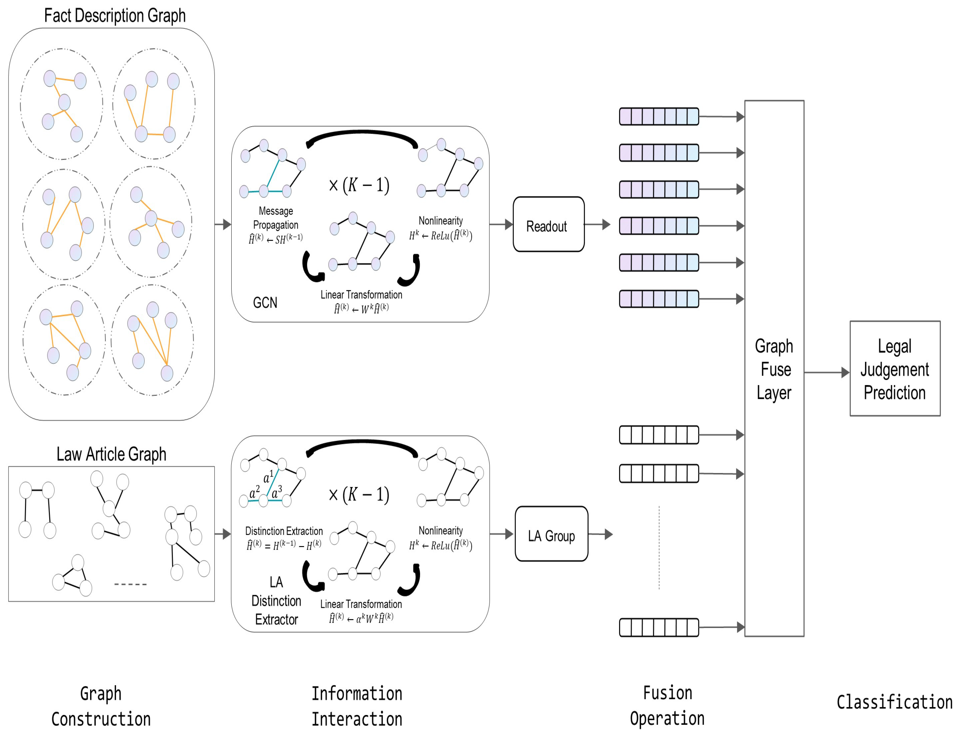
• We propose a method to fuse different feature information of nodes from different kinds of graphs (graph fusion method).
• This paper incorporates six kinds of graphs to predict case judgment; we achieved excellent results using real-world datasets, outperforming all baseline models.

This paper contains five sections in total and the first is an introduction. Section 2 focuses on the related work. In Section 3, the details of the proposed method are presented. In Section 4, the experimental results and analysis of the model are shown. Finally, the entire paper is summarized in Section 5.

2. Related Work

LJP received attention a long time ago, with the earliest work dating back to 1957 with Kort [16]. Existing LJP works can be divided into three categories; the first uses mathematical or statistical methods, which are primarily early work, using some linear classifiers and incorporating legal rules to make such work well interpreted, but they have poor generalization. With the development of deep learning techniques, deep-learning-based methods have been widely applied to LJP tasks.

The second uses the novel architecture of the model to improve the performance of the task. Ref. [17] proposed a model based on the combination of FastText and TextCNN to solve the task. Ref. [18] proposed a hierarchical legal cause prediction (HLCP) model that uses an attention-based end-to-end model to predict charges. Ref. [19] proposed a multi-channel attentive neural network that extracts the case fact description, the defendants and relevant law articles. Ref. [20] proposed a new recursive attention network (RAN) to match fact descriptions and law articles correctly. Ref. [21] devised a new approach based on the judge’s decision process. The method incorporates the plaintiff’s claims and court debate data to reach the final judgment through multi-task learning. Ref. [22] used an gating mechanism-based model to enhance the term of penalty prediction. Ref. [23] proposed a multi-level attention-based model that can handle cases containing multiple defendants.

The third is to explore how to incorporate legal knowledge into the model. Ref. [24] proposed a method to obtain the points related to the fact description from the definition of a charge, which enhances the feature representation of the fact description and improves the performance of the charge prediction task. Ref. [4] used an RNN model based on an attention mechanism and incorporated the information of the relevant law articles into the model. Ref. [6] summarized ten different legal attributes and applied them to the data of less frequent charges to alleviate the poor prediction results of low-frequency charges.

In addition, ref. [25] proposed a large-scale Chinese LJP dataset in 2018, which contains a large number of legal instruments opened by the Chinese government and contains three subtasks, law articles, charges and term of penalty prediction. This dataset also provides a convenient condition for later scholars to engage in research in related fields, which significantly contributes to the development of the field.

3. Our Method

As shown in Figure 2, we propose a graph neural network-based LJP method. Firstly, six kinds of text graph were constructed based on judicial decision documents, including the following: co-occurrence graph, point-wise mutual information (PMI) graph, semantic graph (using cosine similarity, Euclidean distance, Manhattan distance and Chebyshev distance). The nodes in the graph are words of the document, document virtual nodes; they then went through a GCN for intra-graph information passing. For the law article graph, we used the law article (LA) distinction extractor to obtain the information of different point features of similar law articles. Then, we input the text graph features and the law article graph features into the graph fusion layer to predict the results of LJP.

3.1. Problem Formulation

In this section, we briefly describe the fact descriptions, law articles, charges, terms of penalty and legal judgment prediction, as well as the related notations and terminology, as Figure 3:

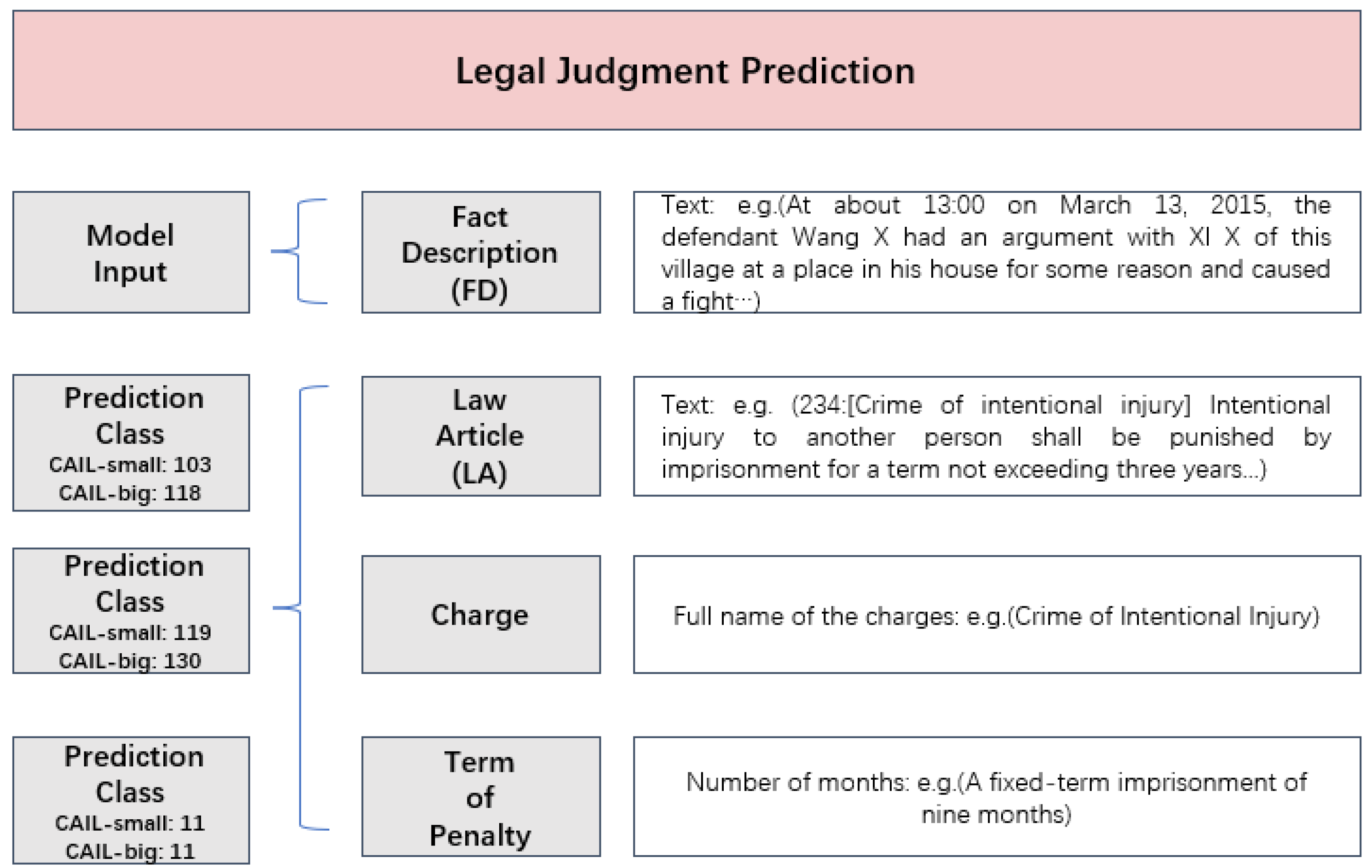
• Fact description: The fact description is a part of an Judicial decision document which mainly describes the time and place of the case, the defendant, what illegal activities were carried out, etc., and is noted as $FD$.
• Law article: Law articles are the basis for convictions and each charge has at least one law article. The law articles are noted as $L=\{L{A}_1,L{A}_2,\dots ,L{A}_n\}$. In the dataset used in the paper, the maximum number is 118.
• Charge: The charges are the items that need to be predicted. The maximum number is 130.
• Term of penalty: The terms of penalty are the items that need to be predicted. The maximum number is 11.
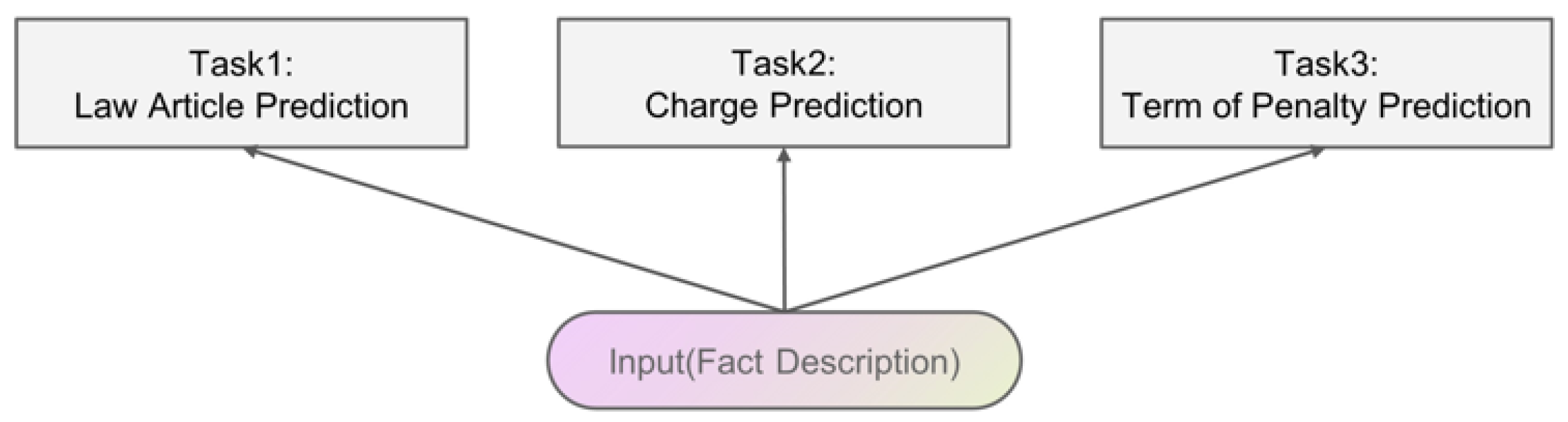
• Legal judgment prediction: The LJP task is to obtain the legal judgment based on the fact description of the case and our task is to train a model F to predict the LJP LJP result (applicable law articles, charges and terms of penalty).

3.2. Graph Construction Based on Legal Text

In this section, we illustrate how to construct six kinds of text graph $G_k(V,E_k)$ for each document, where k denotes the k-th graph of the document and k belongs to $[1,6]$; V represents all graph nodes, including the word or virtual document nodes; and E is the set of the weights of the edges.

3.2.1. Co-Occurrence Graph

Word co-occurrence relationships are often used to analyze research topics in various disciplines and refer to the co-occurrence of several words in the exact text or sentence, or paragraph. When several words frequently appear together, there is likely to be a semantic relation between them. For a pair of words $w_i,w_j$, the edge weights between them are calculated using the following formula:

$$E_{i,j}=p\left(w_j\right|w_i)=\#N(w_i,w_j)/\#N\left(w_i\right)$$

(1)

where $E_{i,j}$ represents the co-occurrence relationship between two words, $\#N\left(w_i\right)$ is the number of occurrences of the word $w_i$ in the co-occurrence window and $\#N(wi,wj)$ is the number of occurrences of the word pair $wi,wj$ in the co-occurrence window. If $\#N(wi,wj)$ is 0, it means that the word pair has no co-occurrence relations.

3.2.2. Point-Wise Mutual Information Graph

PMI is a way to calculate word association, the value of which represents the closeness of the relation between two words. The basic idea of PMI is to count the probability of two words appearing together in the text. If the probability is higher, its relevance is closer and the association is higher. PMI is calculated as follows:

$$\begin{array}{cc}\hfill E_{i,j}=PMI(i,j)& =log\frac{p(i,j)}{p\left(i\right)p\left(j\right)}\hfill \\ \hfill p(i,j)& =\frac{\#NW(i,j)}{\#NW}\hfill \\ \hfill p\left(i\right)& =\frac{\#NW\left(i\right)}{\#NW}\hfill \end{array}$$

(2)

where $\#NW$ is the number of sliding windows defined in the whole dataset, $\#NW(i,j)$ is the number of windows containing word i and word j and $\#NW\left(i\right)$ is the number of sliding windows containing word i. When PMI is positive, the larger its value is, the greater the semantic relevance between two words it represents. When PMI is negative, there are basically no relationships between the two words. Only the edges with positive PMI values are retained in our method and the edges with negative weights are directly discarded.

3.2.3. Semantic Graph

The word vectors are obtained from a pre-trained model based on a large corpus. The pre-trained model has achieved great success in recent years and has broken the list in many NLP tasks, indicating that the pre-trained model has learned the text’s semantic, syntactic and structural information. In our method, we construct four types of word semantic graphs based on Cosine similarity, Euclidean distance, Manhattan distance and Chebyshev distance. The Cosine similarity is a standard similarity calculation method, which uses the cosine of the angle between two vectors in the vector space to measure the difference between two individuals. Compared with the distance metric, Cosine similarity focuses on the difference between two vectors in a direction rather than distance or length. We use the cosine similarity measure to calculate the edge weights of word pairs which corresponds to the following formula:

$$E_{i,j}=sim(i,j)=cos\theta =\frac{x_i·x_j}{|x_i|·|x_j|}$$

(3)

The remaining three ways of constructing graphs are based on distance metrics, which are used to calculate the distance values of individuals (word vectors) present in the space, with larger values indicating more significant differences between individuals [26]. Euclidean distance is the most common distance metric, which measures the absolute distance between word vectors, corresponding to the following equation:

$$E_{i,j}=dist(i,j)=\left|\right|x_i-x_j{\left|\right|}_2$$

(4)

Manhattan distance is a generalization of the Euclidean distance, which is calculated as

$$E_{i,j}=dist(i,j)=\left|\right|x_i-x_j{\left|\right|}_1$$

(5)

where ${\left|\right|a\left|\right|}_1$ means L1 norm, which is the sum of the absolute values of the elements of the vector a; ${\left|\right|a\left|\right|}_2$ means L2 norm, which is the sum of the squares of the elements of the vector a and then the square root.

Chebyshev distance originates from the move of the Chinese king in chess. Chebyshev distance is Ming’s distance when p tends to infinity, which is calculated as

$$E_{i,j}=dist(i,j)=max|x_i-x_j|$$

(6)

3.2.4. Build Graph for Each Document

As mentioned above, we constructed six kinds of graphs for each document and we removed edges with weight values less than 0 or less than the threshold we set. Such an approach can filter some noise and reduce the computational effort when passing information between graphs. Document virtual nodes are linked to all word nodes in the document and the edge weight is 1. For these six types of graph, we denoted $G_s={(V,E_s)}_{s=1}^6$.

3.3. Law Article Distinction Extractor

3.3.1. Build Law Articles Graph

We treated the law articles as nodes and the edge weights between nodes were the cosine similarity of the document representation vector $(V_{li},V_{lj})$ of the law article pairs. $V_{li},V_{lj}$ were obtained as a weighted average for each Glove word embedding in the sentence using tf-idf. Here, we set a threshold p to filter out the edges with weights less than p in the graph, so the law article graph was divided into m groups (supposing the number is m). The law articles within each group had similarities at the semantic level.

3.3.2. Law Article Groups’ Distinct Learning Operation

The graph constructed in the previous step could distinguish the different law article groups, but distinguishing similar law articles in one group is the critical problem. In order to better distinguish the similar law article in the same group, we propose a law distinction learning operation inspired by the graph attention network (GAT) [27]. Our approach differs from GAT in that we use an attention-based mechanism to remove the similarity information between each law article node. This operation can preserve the unique feature information of each law article and thus can distinguish similar law articles. The specific formula is as follows:

$$V_{L_i}^{\left(l\right)}=W^{(l-1)}{V}_{l-1}^{L_i}-\frac{1}{K}\sum _{k=1}^K\sum _{j\in N_i}{\alpha }_{ij}^k{W}^k{V}_j$$

(7)

$${\alpha }_{ij}=\frac{exp\left(LeakyReLU\right({\beta }^T[W{V}_i\left|\right|W{V}_j\left]\right))}{{\sum }_{j\in N_j}exp\left(LeakyReLU\right({\beta }^T[W{V}_i\left|\right|W{V}_j\left]\right))}$$

(8)

where $V^{\left(l\right)}$ refers to the representation of law article $L_i$ in the l-th layer; $N_j$ refers to the neighbor set of $L_i$ in graph G; and $W_l$ and $W_k$ are the trainable self-weighted matrix and the neighbor similarity extracting matrix, respectively. ${\alpha }_{ij}$ indicates the importance of node j for node i and node i must be the first-order neighbor of node j. In calculating the attention value between nodes, masked attention is used to achieve the above assumptions. The attention mechanism used in this paper was implemented by a single-layer feedforward neural network, in which the activation function was the $LeakyReLU$ function. The GAT also incorporates a multi-headed attention mechanism, with K representing K heads in the formula.

Then, we used the last layer of the network as a vector representation of the law article nodes, denoted as $V^{\left(l\right)}$. This vector contained information about the different points of similar law articles. For each of the N groups, which were divided in the law article graph, we computed the representation vector separately, with the following equation:

$$h_n=W_d{V}_{L_i}^L+b^{\left(d\right)}$$

(9)

where $W_d$ is a trainable parameter matrix, $n\in N$ and $h_n$ represents the vector representation of the n-th law article group.

3.4. Fact Description Graph Interaction

We used a graph convolutional network (GCN) to encode the nodes for each graph. A GCN acts directly on the graph and can obtain the feature vectors of its nodes from the information of the nodes’ neighbors. All the nodes in the graph are connected to themselves. Let us assume that matrix X contains the features of all n nodes in the graph, where m is the dimension of the feature vector of each node. The matrix A is the adjacency matrix of G and D is the degree matrix of G and the values on the diagonal of A are all 1. The GCN can obtain the information of direct neighbor nodes after the first layer of the graph convolution operation. When multiple layers of GCNs are stacked, the information of a more extensive range of neighbors can be learned. When the initial node feature matrix is calculated by one layer of GCN, the k-dimensional node feature matrix $L^{\left(1\right)}\in {\mathbf{R}}^{n\times k}$ is obtained, which is calculated as follows:

$$L^{\left(1\right)}=tanh\left(\tilde{A}X{W}_0\right)$$

(10)

where $\tilde{A}=D^{-1/2}A{D}^{-1/2}$ is the normalized symmetric adjacency matrix and $W_0$ is the parameter matrix. The hyperbolic tangent function (tanh) is used for the activation function based on experiment. For multilayer GCN calculation,

$$L^{(p+1)}=tanh\left(\tilde{A}{L}^{\left(p\right)}{W}_p\right)$$

(11)

where p is the number of layers, $L^{\left(0\right)}=X$. We chose to use a three-layer GCN as the graph feature extractor. Based on the experiments performed in this paper, we show that the three-layer GCN could make the node information pass well and the one-layer and multi-layer GCNs were worse than the three-layer GCN.

Then, we used the following readout functions for the six kinds of graph of one document:

$$L_v=sigmoid\left(W_1{L}_v^l\right)\odot tanh\left(W_2{L}_v^l\right)$$

(12)

$$h_G=Averagepooling(L_1...L_V)+Maxpooling(L_1...L_V)-Minpooling(L_1...L_V)$$

(13)

where $L_v$ is the graph node feature calculated by the attention mechanism. We then used Averagepooling to add with Maxpooling and subtract with Minpooling. The idea is that each text word contributes to the task, with essential words contributing more information and unimportant words potentially having a negative effect.

3.5. Graph Fusion Layer

After the calculation of the above steps, for each document, we obtained six different levels of vector expressions; then, we concatenated the six vectors as follows:

$$H=\underset{s=1}{\overset{6}{\left|\right|}}{h}_G^s$$

(14)

where $\left|\right|$ is the concatenation operation; in order to incorporate different vector representations, we designed the fusion method for fact description graphs with the following equation:

$$\alpha =softmax(w^{T}tanh\left(H\right))$$

(15)

$$H^{*}=H{\alpha }^T$$

(16)

where w is the trainable parameter and $\alpha$ is the weight vector of H. After that, we mixed the information of the law article group into the model. This part of our designed idea is also to use the attention mechanism so that the model can use the importance of the law article group for dynamic selection so that, in this step, we fuse the features of the six types of graph and add the features of the law article. The formula is as follows:

$$\alpha =softmax(tanh{\left(W{H}^{*}\right)}^T\left(W_L{h}_N\right))$$

(17)

$$H^F=\alpha H^{*}$$

(18)

where $W_L$ and W are trainable weight matrices. Then, we obtained a representation of graph fusion, where $H^F$ denotes the vector before the classification layer.

3.6. Prediction and Train

Here, we have three subtasks, t1, charge prediction; t2, sentence prediction; and t3, law prediction. We used the $H^F$ obtained in the previous step and input it into the softmax classifier as follows:

$${\widehat{y}}_j=softmax(W_p^j{H}^F+b_p^j)$$

(19)

where $W_p^j$ and $b_p^j$ are parameters specific to task $t_j$. For training, we computed a cross-entropy loss function for each subtask and took the loss sum of all subtasks as the overall prediction loss.

$${\mathbf{L}}_p=-\sum _{j=1}^3\sum _{k=1}^{|Y_j|}{y}_{j,k}log\left({\widehat{y}}_{j,k}\right)$$

(20)

where $|Y_j|$ denotes the number of different labels for task $t_j$ and ${\widehat{y}}_{j,k}$ refers to the ground-truth vector of task $t_j$.

4. Experiments

To validate our method, we conducted rich experiments to verify the performance of the model. We selected all three subtasks of LJP, including charge, term of penalty and law article prediction.

4.1. Datasets

We used the Chinese AI and Law challenge (CAIL2018) dataset to validate the performance of our model. CAIL2018 contains two parts of data, CAIL-small (practice phase data) and CAIL-big (main competition phase data), and each sample in the dataset contains a text of case fact description, relevant law articles, charges and terms of penalty. In the pre-processing data stage, we first filtered out samples with a length of fact description text less than 10, then filtered out samples with only a single charge and single law article and, finally, removed data with sample size less than 100. We took about 15% of the total data as the test set and the rest as the training set. The

Table 1. Dataset details.

Dataset	CAIL-Small	CAIL-Big
Training Set Cases	101,690	1,588,768
Test Set Cases	20,338	185,212
Law Articles	103	118
Charges	119	130
Terms of Penalty	11	11

below shows the detailed statistical information of the dataset used in experiments.

4.2. Baselines

• TFIDF + SVM: This technique uses TF-IDF to make text vectors and SVM [28] as a text classifier.
• CNN [29]: This method uses CNNs containing multiple filters and employs softmax as a classifier.
• RCNN [30]: The approach fuses RNN and CNN to make a new model and exploits the advantages of both models to improve the performance of text classification.
• HARNN [31]: First, the method considers the hierarchical structure of documents; words form sentences and sentences form documents, so the modeling is also performed in these two parts and the attention mechanism is introduced.
• FLA [2]: The method proposes an attention-based neural network framework that can perform the task of charge prediction and relevant law articles extraction and show the importance of law articles in the civil law system for judicial decision making.
• TOPJUDGE [32]: The approach unifies multiple subtasks of LJP into a single learning framework, builds dependencies between LJP subtasks into a DAG form and enhances trial predictions using prior knowledge. The model can handle any DAG-dependent subtasks.
• GCN [12]: This method uses text to construct a graph and then a graph convolutional network to extract node features for classification.
• MPBFN-WCA [2]: The approach designs a multi-view forward prediction and backward verification framework to efficiently exploit the dependencies between multiple subtasks. The word matching features of fact descriptions are integrated into the network through an attention mechanism to distinguish cases with similar descriptions but different penalties.
• LADAN [8]: The model effectively solves the problem of confusing charges (law articles) in the LJP task. The method takes into account not only the positive effect of the textual definitions of charges (law articles) on the semantic extraction of case fact descriptions but also the negative effect of interrelationships (e.g., similarity relations) between the definitions of charges (law articles) on the semantic extraction.

4.3. Experimental Settings

The datasets of test and validation for the experiments are shown in Section 4.1. We used THULAC for word segmentation, which is excellent in handling Chinese segmentation. We used the Glove model [33] to pre-train the word vectors, where the word vectors were set to 300 dimensions. For the CNN-based comparison model, we set the maximum document length to 512 and, for the RNN-based comparison model, we set the maximum number of words in a sentence to 150 and the maximum number of sentences in a document to 15. Based on the preliminary experimental results on evaluation tests, we used the Adam optimizer [34] with a learning rate of 0.01 and set the dropout to 0.5. The GCN interaction steps were three and the sliding window size was 3. To reduce the memory overhead, we used mini-batch for training. The environment of hardware and software of the experiment are shown in

Table 2. Hardware environment.

Hardware Name	Parameter Description	Quantity
CPU	Intel Core i7-10700K	2
GPU	NVIDIA Tesla V100 32 G	1
Memory	Lenovo 16 G	2
SSD	SAMSUNG 512 G	1
Hard Disk	Seagate 1 TB	2

and

Table 3. Software environment.

Software Name	Parameter Description
$\mathrm{Operating}\mathrm{system}$	Ubuntu 16.04
$\mathrm{Development}\mathrm{tool}$	Pycharm 2020
$\mathrm{Version}\mathrm{of}\mathrm{Python}$	3.8
$\mathrm{Version}\mathrm{of}\mathrm{Pytorch}$	1.7.0
$\mathrm{Version}\mathrm{of}\mathrm{DGL}$	0.3

.

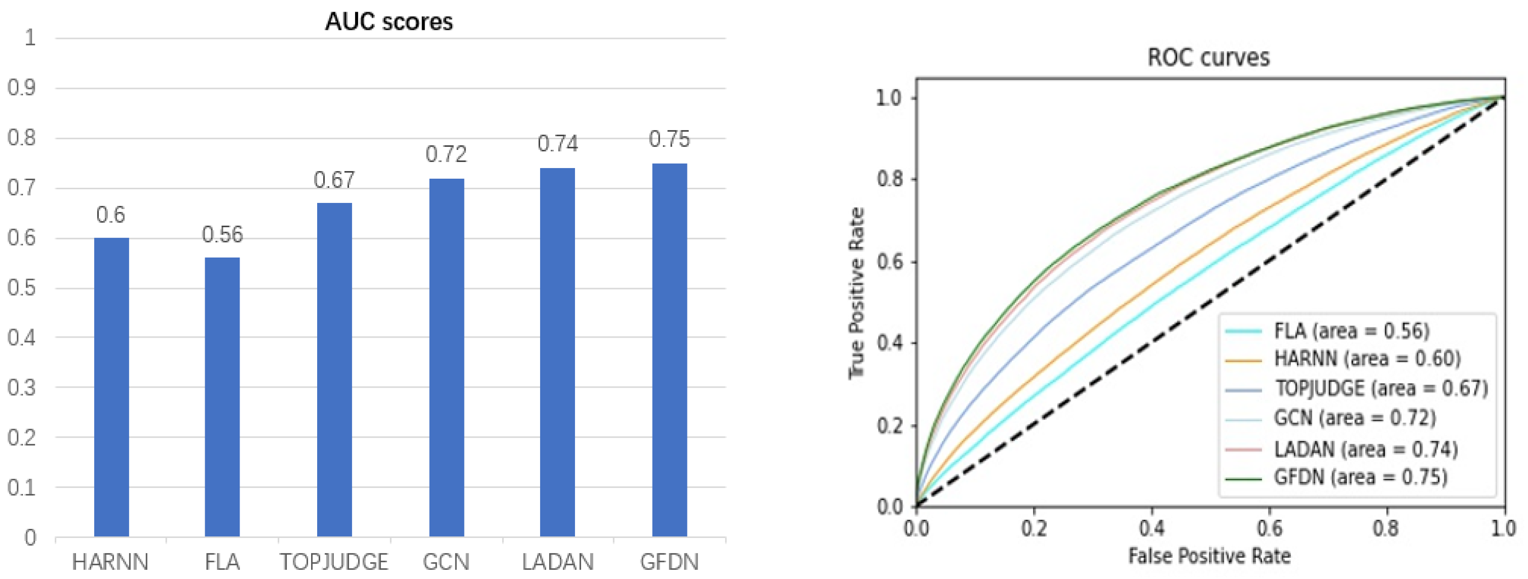
4.4. Experimental Results

We chose four metrics (accuracy, macro-precision, macro-recall and macro-F1) to compare the performance of our model with the baseline model on the task. We used a multi-task approach for each baseline model to train the model and select the best set of parameters as the experimental results. All models were trained five times and we selected their average values as the data results used for comparison.

Our method is noted as GFDN.

Table 4. LJP results on dataset CAIL-big.

	Law Articles				Charges				Term of Penalty
	Acc.	MP	MR	F1	Acc.	MP	MR	F1	Acc.	MP	MR	F1
TFIDF + SVM	89.93	68.56	60.58	61.25	85.81	69.76	61.92	63.51	54.13	39.15	37.62	39.14
FLA	93.22	72.81	64.27	66.57	92.48	76.21	68.12	69.97	57.66	49.01	44.87	46.62
CNN	95.79	82.79	75.15	76.62	95.23	86.57	78.93	81.02	55.41	45.23	38.73	39.96
RCNN	95.98	82.93	75.26	77.13	95.50	87.89	79.03	81.65	55.62	45.43	38.88	40.17
HARNN	96.01	82.99	75.58	77.38	95.62	87.93	79.27	81.79	56.11	44.21	40.57	41.87
TOPJUDGE	95.81	84.41	74.36	76.67	95.73	87.99	79.49	81.93	57.29	47.35	42.61	44.03
GCN	95.69	84.24	74.22	76.58	95.60	87.89	79.28	81.82	57.2	47.17	42.53	43.91
MPBFN	96.01	84.83	74.64	77.48	95.93	89.25	80.82	83.06	58.04	45.95	39.01	41.49
LADAN	96.49	85.71	80.21	81.35	96.32	88.03	82.98	84.54	59.52	51.83	45.2	46.96
GFDN	96.51	85.74	80.23	81.39	96.42	88.05	83.12	84.64	59.54	51.84	45.21	46.99

and

Table 5. LJP results on dataset CAIL-small.

	Law Articles				Charges				Term of Penalty
	Acc.	MP	MR	F1	Acc.	MP	MR	F1	Acc.	MP	MR	F1
TFIDF + SVM	76.52	43.21	40.12	39.68	79.81	45.86	42.72	42.77	33.32	27.66	24.99	24.64
FLA	77.72	75.21	74.12	72.78	80.98	79.11	77.92	76.77	36.32	30.81	28.22	27.83
CNN	78.61	75.86	74.6	73.59	82.23	81.57	79.73	78.82	35.2	32.96	29.09	29.68
RCNN	79.12	76.58	75.13	74.15	82.50	81.89	79.72	79.05	35.52	33.76	30.41	30.27
HARNN	79.73	75.05	76.54	74.67	83.41	82.23	82.27	80.79	35.95	34.5	31.04	31.18
TOPJUDGE	79.79	79.52	73.39	73.33	82.03	83.14	79.33	79.03	36.05	34.54	32.49	29.19
GCN	79.81	79.65	73.42	73.37	82.33	83.19	79.20	78.97	35.97	34.66	32.54	29.23
MPBFN	79.14	76.03	71.1	72.21	82.16	83.15	80.82	80.06	35.76	31.72	28.31	29.56
LADAN	81.17	77.92	72.43	73.79	84.02	83.18	82.08	81.04	38.05	35.97	32.15	32.33
GFDN	81.37	78.01	72.43	73.82	84.83	83.96	82.37	81.79	38.28	36.02	32.28	32.57

show the experimental results on the datasets CAIL-big and CAIL-small, respectively. It can be concluded that our method was better than the baseline models in all metrics. Compared with LADAN, which is the best performing baseline model, the performance of our model on the CAIL-big dataset was improved by 0.1%, 0.02%, 0.14% and 0.1% and by 0.81%, 0.78%, 0.29% and 0.75% in the CAIL-small dataset, respectively, in terms of accuracy, precision, recall and F1-value in the charge prediction task. In the law article prediction task, our model improved by 0.02%, 0.03%, 0.02% and 0.04% on the CAIL-big dataset and by 0.2%, 0.09%, 0% and 0.03% on the CAIL-small dataset, respectively; in the term of penalty prediction task, our model improved by 0.02%, 0.01%, 0.03% and 0.02% on the CAIL-big dataset and by 0.23%, 0.05%, 0.13% and 0.24% on the CAIL-small dataset, respectively. The main reasons why our model achieved excellent experimental results can be attributed to two points. First, the six kinds of text graphs not only could use the GCN well to obtain text-level feature information but could also obtain inferred information that traditional text feature extraction methods cannot obtain. The graph structure has a natural advantage in inference. Second, the proposed law article distinction extractor could well extract the differences of similar law articles and could also well integrate the information with six kinds of graphs in the graph fusion step. From the analysis in Table 5, we can see that our model also showed excellent performance when dealing with small-sample datasets. The model showed a significant improvement over the LADAN model on CAIL-small. The main reason is that traditional neural network methods require a large number of data as the basis. Our method is based on a graph neural network, which has some advantages in dealing with small-sample datasets according to the experimental results. In predicting the law articles on CAIL-small, our method did not achieve optimal results. The possible reason is that the law articles distinction extractor hurt the model’s performance in predicting law articles in a dataset with few samples. In addition, we could also infer, from the two tables, that the number of data in LJP directly determined the performance of the task (all models performed much better on CAIL-big than CAIL-small). The main reason is that the performance of a deep learning model depends heavily on the number of training data and the same is true for the LJP task.

Since the data gap between Table 4 and Table 5 is relatively small, we conducted statistical significance tests and the results are shown in Figure 4. We assumed the null hypothesis as no significant differences between the two groups of data and the alternative hypothesis as a significant difference. As shown in Figure 4, the red dots are the distribution of the samples. The t value fell in the rejection domain, so we rejected the null hypothesis and accepted the alternative hypothesis that there was a significant difference between the two data groups. Then, the Wilcoxon test was also performed in our experiment. In the CAIL-big dataset, we assumed that there were no differences between the experimental results of GFDN and LADAN. Based on the calculated p-value (p = 0.003857 < 0.005), the original hypothesis was rejected; therefore, it can be concluded that there was a significant difference between the two sets of experimental data. Both sets of experiments illustrated that our method was significantly better than the LADAN in terms of performance.

In the CAIL-big dataset, there is data imbalance. We plotted the ROC curves and show the corresponding AUC scores because they considers the classification ability for both positive and negative cases. It could still make a reasonable classifier evaluation in such a case. We selected five models from the baseline to compare the AUC with our model GFDN. From Figure 5, we can see that the FLA model had the lowest AUC score because its semantic extractor was not powerful enough to extract the document information fully. Although FLA was designed for the LJP task, it had a lower AUC score than the HARNN model. The TOPJUDGE model did not address this problem accordingly, so its AUC score was also low. GCN, LADAN and GFDN all contain graph neural networks and GFDN uses multiple methods to construct text graphs, which allowed the model to fully extract feature information and alleviate the problem of data imbalance.

Although the metrics presented are an average of the results obtained from five runs, providing only the average value is still insufficient to determine whether the observed differences are robust or occur by chance. Therefore, we show the minimum and maximum metrics from our methods’ runs and compare them with the results of LADAN. In

Table 6. Maximum and minimum values of LJP experimental results.

	Accuracy		Precision		Recall		F1
	Max	Min	Max	Min	Max	Min	Max	Min
$\mathrm{Law}{\mathrm{Articles}}_{big}$	96.53 ↑	96.50↑	85.77↑	85.73↑	80.25↑	80.21-	81.43↑	81.37↑
$\mathrm{Law}{\mathrm{Articles}}_{small}$	81.50 ↑	81.21 ↑	78.12 ↑	77.95 ↑	72.52 ↑	72.41 ↓	73.85 ↑	73.80 ↑
${\mathrm{Charges}}_{big}$	96.46↑	96.39↑	88.08↑	88.04↑	83.19↑	83.06↑	84.78↑	84.59↑
${\mathrm{Charges}}_{small}$	85.12↑	84.61↑	84.27↑	83.36↑	82.48↑	82.15↑	81.92↑	81.35↑
$\mathrm{Terms}\mathrm{of}{\mathrm{Penalty}}_{big}$	59.57↑	59.52-	51.87↑	51.83-	45.23↑	45.19↓	47.03↑	46.96-
$\mathrm{Terms}\mathrm{of}{\mathrm{Penalty}}_{small}$	38.35↑	38.19↑	36.12↑	35.98↑	32.37↑	32.21↑	32.68↑	32.46↑

, we used ↓ if the value was less than LADAN, ↑ if the value was more significant than LADAN and − if it was equal. From Table 6, we can see that most of the minimum values of our method are larger than the average values of LADAN. We can conclude that GFDN was better than LADAN in terms of performance.

4.5. Ablation Experiments

We designed the relevant ablation experiments which used the same comparison metric. First, we designed experiments for the text graph types by subtracting one of the text graphs in turn.

Table 7. Graph ablation experiment results on dataset CAIL-small.

Metrics	Acc	MR	MR	F1
GFDN	84.83	83.96	82.37	81.79
${\mathrm{GFDN}}_{(-CO)}$	82.35	83.27	79.37	79.91
${\mathrm{GFDN}}_{(-PMI)}$	82.40	83.19	80.28	80.52
${\mathrm{GFDN}}_{(-COS)}$	82.58	83.29	80.37	80.83
${\mathrm{GFDN}}_{(-Euclidean)}$	82.69	83.35	80.51	80.91
${\mathrm{GFDN}}_{(-Manhattan)}$	82.67	83.30	80.77	80.93
${\mathrm{GFDN}}_{(-Chebyshev)}$	82.69	83.38	80.55	80.96

shows the results of this experiment and we can see that the impact of the graph without co-occurrence graph experiment was the largest, which indicates that the co-occurrence graph contained more information about the features that could be used in this task. The impact of the missing Cosine graph, Euclidean graph, Manhattan graph and Chebyshev graph on the results was less than that of the PMI graph, which indicates that we could pursue the model’s efficiency using only one of the similarity calculation methods for constructing the graph.

We also conducted experiments in the graph fusion section, where we used simple concatenation and took an average. As we can see in

Table 8. Fusion ablation experiment results on dataset CAIL-small.

Metrics	Acc	MR	MR	F1
GFDN	84.83	83.96	82.37	81.79
${\mathrm{GFDN}}_{Concatenation}$	81.96	80.38	79.11	79.32
${\mathrm{GFDN}}_{Average}$	80.67	79.96	80.13	79.06

, the experimental results indicate that our approach achieved the best results. The simple concatenation and averaging approaches destroyed the feature information and degraded the model’s performance.

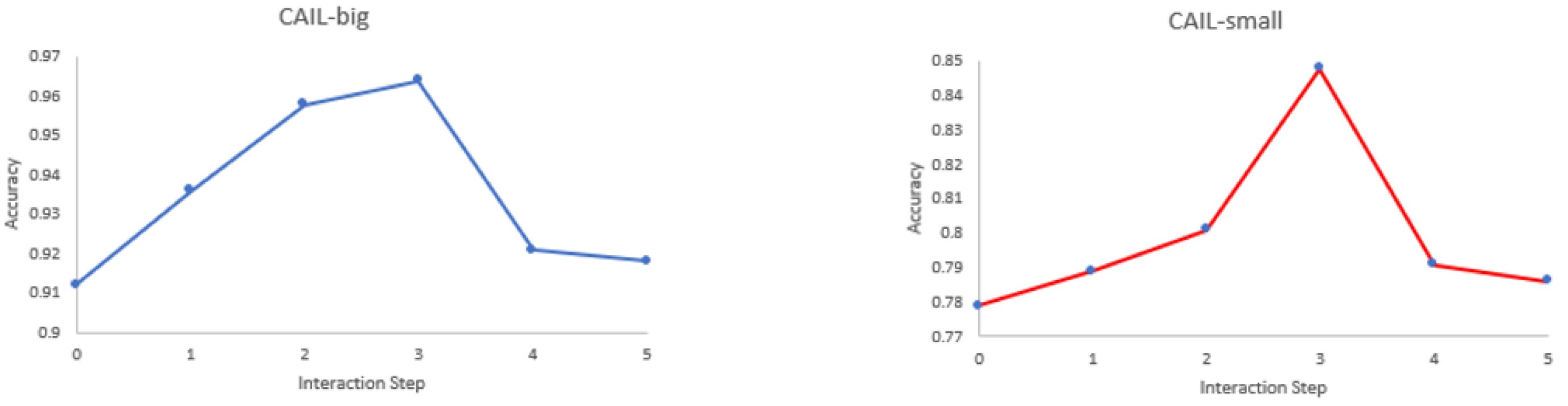
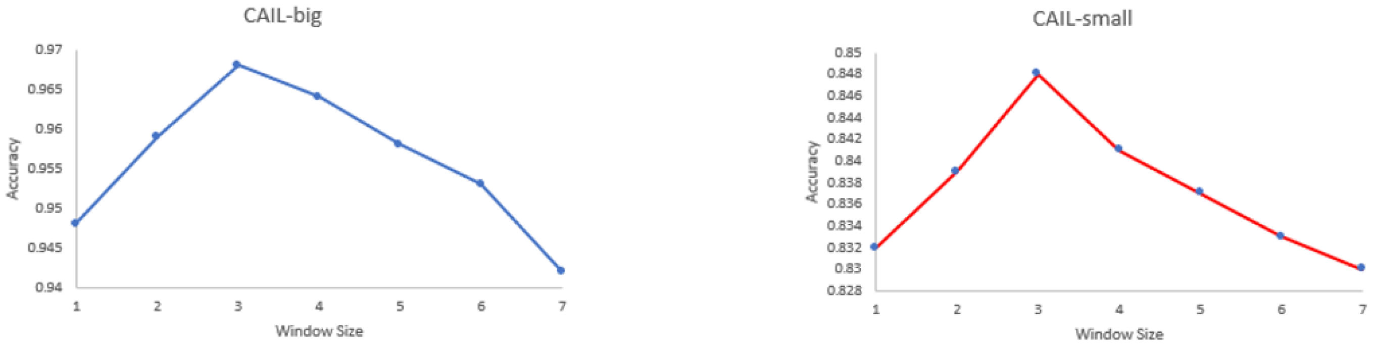
4.6. Parameter Sensitivity

We performed this experiment for the number of iterations and co-occurrence window size selection of GCN. We only compared the accuracy in the charge prediction task. First, we selected the number of iterations of the GCN as one, two, three, four and five. From the Figure 6, we can see that the best result was achieved with three iterations. The curve shows a rising and then decreasing trend, which indicates that, after three iterations, the model experienced an over-fitting phenomenon.

We chose, as one, two, three, four, five and six, the set of parameters for the co-occurrence window size and it can be seen from the Figure 7 that a window size of three achieved the best results. The curve shows a rising and then decreasing trend, indicating that the model reached over-fitting after the window size of three.

5. Conclusions

We propose an inductive legal judgment prediction method based on graph neural networks. The method first constructs six kinds of text graphs for each document and then uses graph convolutional networks to transfer and update information within the text graphs to fully understand and extract feature information of documents of the judicial case. we also utilize an improved legal text differentiation extractor based on graph attention network to obtain the information about the differences of law articles between similar charges. In the graph fusion stage, we mixed the document features of the six kinds of text graphs and law articles information that carried the differentiated features. The experimental results show that our method performed well and achieved good results in all three subtasks of the legal judgment prediction task. Our future work is divided into two parts. First, we will investigate new methods for constructing graphs from texts, including information from multiple dimensions. Second, more efficient graph fusion methods with external knowledge will be adopted to improve the performance of multiple tasks in legal intelligence, including legal judgment prediction (LJP).

References

1. Zhong, H.; Xiao, C.; Tu, C.; Zhang, T.; Liu, Z.; Sun, M. How Does NLP Benefit Legal System: A Summary of Legal Artificial Intelligence. In Proceedings of the 58th Annual Meeting of the Association for Computational Linguistics, Online, 5–10 July 2020; pp. 5218–5230. [Google Scholar]
2. Yang, W.M.; Jia, W.J.; Zhou, X.J.; Luo, Y.T. Legal Judgment Prediction via Multi-Perspective Bi-Feedback Network. In Proceedings of the Twenty-Eighth International Joint Conference on Artificial Intelligence, Macao, China, 10–16 August 2019; pp. 4085–4091. [Google Scholar]
3. Beltagy, I.; Peters, M.E.; Cohan, A. Longformer: The long-document transformer. arXiv 2020, arXiv:2004.05150. [Google Scholar]
4. Kitaev, N.; Kaiser, L.; Levskaya, A. Reformer: The Efficient Transformer. In Proceedings of the International Conference on Learning Representations, New Orleans, LA, USA, 6–9 May 2019; pp. 1–10. [Google Scholar]
5. Wang, S.; Li, B.Z.; Khabsa, M.; Fang, H.; Ma, H. Linformer: Self-attention with linear complexity. arXiv 2020, arXiv:2006.04768. [Google Scholar]
6. Choromanski, K.M.; Likhosherstov, V.; Dohan, D.; Song, X.; Gane, A.; Sarlos, T.; Hawkins, P.; Davis, J.Q.; Mohiuddin, A.; Kaiser, L.; et al. Rethinking Attention with Performers. In Proceedings of the International Conference on Learning Representations, Addis Ababa, Ethiopia, 30 April–2 May 2020; pp. 1–9. [Google Scholar]
7. Zaheer, M.; Guruganesh, G.; Dubey, K.A.; Ainslie, J.; Alberti, C.; Ontanon, S.; Pham, P.; Ravula, A.; Wang, Q.; Yang, L.; et al. Big bird: Transformers for longer sequences. Adv. Neural Inf. Process. Syst. 2020, 33, 83–97. [Google Scholar]
8. Tay, Y.; Dehghani, M.; Abnar, S.; Shen, Y.; Bahri, D.; Pham, P.; Rao, J.; Yang, L.; Ruder, S.; Metzler, D. Long Range Arena: A Benchmark for Efficient Transformers. In Proceedings of the International Conference on Learning Representations, Addis Ababa, Ethiopia, 30 April–2 May 2020; pp. 10–17. [Google Scholar]
9. Niklaus, J.; Chalkidis, I.; Stürmer, M. Swiss-Judgment-Prediction: A Multilingual Legal Judgment Prediction Benchmark. arXiv 2021, arXiv:2110.00806. [Google Scholar]
10. Chalkidis, I.; Jana, A.; Hartung, D.; Bommarito, M.; Androutsopoulos, I.; Katz, D.M.; Aletras, N. LexGLUE: A Benchmark Dataset for Legal Language Understanding in English. arXiv 2021, arXiv:2110.00976. [Google Scholar] [CrossRef]
11. Xiao, C.; Hu, X.; Liu, Z.; Tu, C.; Sun, M. Lawformer: A pre-trained language model for chinese legal long documents. AI Open 2021, 1, 79–84. [Google Scholar] [CrossRef]
12. Luo, B.; Feng, Y.; Xu, J.; Zhang, X.; Zhao, D. Learning to predict charges for criminal cases with legal basis. In Proceedings of the 2017 Conference on Empirical Methods in Natural Language Processing, Copenhagen, Denmark, 7–11 September 2017; pp. 2727–2736. [Google Scholar]
13. Hu, Z.; Li, X.; Tu, C.; Liu, Z.; Sun, M. Few-shot charge prediction with discriminative legal attributes. In Proceedings of the 27th Conference on Computational Linguistics and Speech Processing, Santa Fe, NM, USA, 20–26 August 2018; pp. 487–498. [Google Scholar]
14. Xu, N.; Wang, P.; Chen, L. Distinguish Confusing Law Articles for Legal Judgment Prediction. In Proceedings of the 58th Annual Meeting of the Association for Computational Linguistics, Online, 5–10 July 2020; pp. 3086–3095. [Google Scholar]
15. Kipf, T.; Welling, M. Semi-supervised classification with graph convolutional networks. In Proceedings of the 2017 International Conference on Learning Representations, Toulon, France, 24–26 April 2017; pp. 1–14. [Google Scholar]
16. Kort, F. Predicting supreme court decisions mathematically: A quantitative analysis of the right to counsel cases. Am. Political Sci. Rev. 1957, 51, 1–12. [Google Scholar] [CrossRef]
17. Wang, H.; He, T.; Zou, Z.; Shen, S.; Li, Y. Using case facts to predict accusation based on deep learning. In Proceedings of the QRS-C, Sofia, Bulgaria, 22–26 April 2019; pp. 133–137. [Google Scholar]
18. Liu, Z.; Tu, C.; Sun, M. Legal cause prediction with inner descriptions and outer hierarchies. In Proceedings of the Chinese Computational Linguistics, Beijing, China, 17–20 October 2019; pp. 573–586. [Google Scholar]
19. Li, S.; Zhang, H.; Ye, L.; Guo, X.; Fang, B. Mann: A multichannel attentive neural network for legal judgment prediction. IEEE Access 2019, 7, 151144–151155. [Google Scholar] [CrossRef]
20. Yang, Z.; Wang, P.; Zhang, L.; Shou, L.; Xu, W. A recurrent attention network for judgment prediction. In Proceedings of the International Conference on Artificial Neural Networks, Munich, Germany, 17–19 September 2019; pp. 253–266. [Google Scholar]
21. Ma, L.; Zhang, Y.; Wang, T.; Liu, X.; Ye, W.; Sun, C.; Zhang, S. Legal Judgment Prediction with Multi-Stage Case Representation Learning in the Real Court Setting. In Proceedings of the ACM SIGIR, Online, 11–15 July 2021; pp. 993–1002. [Google Scholar]
22. Chen, H.; Cai, D.; Dai, W.; Dai, Z.; Ding, Y. Charge-Based Prison Term Prediction with Deep Gating Network. In Proceedings of the 2019 Conference on Empirical Methods in Natural Language Processing and the 9th International Joint Conference on Natural Language Processing, Hong Kong, China, 3–7 November 2019; pp. 6361–6366. [Google Scholar]
23. Pan, S.; Lu, T.; Gu, N.; Zhang, H.; Xu, C. Charge prediction for multidefendant cases with multi-scale attention. In Proceedings of the CCF Conference on Computer Supported Cooperative Work and Social Computing, Kunming, China, 16–18 August 2019; pp. 766–777. [Google Scholar]
24. Kang, L.; Liu, J.; Liu, L.; Shi, Q.; Ye, D. Creating auxiliary representations from charge definitions for criminal charge prediction. arXiv 2019, arXiv:1911.05202. [Google Scholar]
25. Xiao, C.; Zhong, H.; Guo, Z.; Tu, C.; Liu, Z.; Sun, M.; Feng, Y.; Han, X.; Hu, Z.; Wang, H.; et al. Cail2018: A large-scale legal dataset for judgment prediction. arXiv 2018, arXiv:1807.02478. [Google Scholar]
26. Jafar, O.; Ramakrishnan, S. A Study of Bio-inspired Algorithm to Data Clustering using Different Distance Measures. Int. J. Comput. Appl. 2013, 66, 33–44. [Google Scholar]
27. Velickovic, P.; Cucurull, G.; Casanova, A.; Romero, A.; Li, P.; Bengio, Y. Graph Attention Networks. In Proceedings of the 6th International Conference on Learning Representations, Vancouver, QC, Canada, 30 April–3 May 2018. [Google Scholar]
28. Suykens, J.; Vandewalle, J. Least squares support vector machine classifiers. Neural Process. Lett. 1999, 9, 293–300. [Google Scholar] [CrossRef]
29. Yoon, K. Convolutional neural networks for sentence classification. In Proceedings of the 2014 Conference on Empirical Methods in Natural Language Processing, Doha, Qatar, 25–29 October 2014; pp. 1746–1751. [Google Scholar]
30. Lai, S.; Xu, L.; Liu, K. Recurrent convolutional neural networks for text classification. In Proceedings of the 29th National Conference on Artificial Intelligence, Austin, TX, USA, 25–29 January 2015; pp. 2267–2273. [Google Scholar]
31. Yang, Z.; Yang, D.; Dyer, C. Hierarchical Attention Networks for Document Classification. In Proceedings of the 2016 Conference of the North American Chapter of the Association for Computational Linguistics: Human Language Technologies, San Diego, CA, USA, 12–17 June 2016; pp. 1480–1489. [Google Scholar]
32. Zhong, H.; Guo, Z.; Tu, C.; Liu, Z.; Sun, M. Legal Judgment Prediction via Topological Learning. In Proceedings of the 2018 Conference on Empirical Methods in Natural Language Processing, Brussels, Belgium, October 31–4 November 2018; pp. 3540–3549. [Google Scholar]
33. Pennington, J.; Socher, R.; Manning, C. Glove: Global vectors for word representation. In Proceedings of the 2014 Conference on Empirical Methods in Natural Language Processing, Doha, Qatar, 25–29 October 2014; pp. 1532–1543. [Google Scholar]
34. Kingma, D.P.; Ba, J. Adam: A method for stochastic optimization. In Proceedings of the 3rd International Conference on Learning Representations, San Diego, CA, USA, 7–9 May 2015. [Google Scholar]
Figure 1. Legal judgment prediction.
Applsci 12 02531 g001
Figure 2. Overview of our LJP method.
Applsci 12 02531 g002
Figure 3. An example of LJP. The model’s input is fact description and we need to predict law articles, charges and terms of penalty. The number of classes for the three tasks on the CAIL-small dataset are 103, 119 and 11; the number on the CAIL-big dataset are 118, 130 and 11.
Applsci 12 02531 g003
Figure 4. Statistical significance test results between GFDN and LADAN.
Applsci 12 02531 g004
Figure 5. AUC scores and ROC curves of several models on CAIL-big.
Applsci 12 02531 g005
Figure 6. Effect of different numbers of interactions on accuracy.
Applsci 12 02531 g006
Figure 7. Effect of different window sizes on accuracy.
Applsci 12 02531 g007