Particle Filter Design for Robust Nonlinear Control System of Uncertain Heat Exchange Process with Sensor Noise and Communication Time Delay

Abstract

In this paper, a particle filter design scheme for a robust nonlinear control system of uncertain heat exchange process against noise and communication time delay is presented. The particle filter employs a cluster of particles and associated weights to approximate the posterior distribution of states and is capable of handling nonlinear and non-Gaussian issues. However, when the realistic given noise is much larger than that of the one modeled by the particle filter, the estimated posterior distribution is no longer reliable. Considering that, the exponential weights take the place of the original absolute particle weights in this paper, which act as an adjustment to the particle filter weights for a better state estimation. This adjustment for the weight of the particle filter takes into account the practical significance and can ensure the stability, tracking performance, and continuous operation of the control process incorporated with the particle filter. The simulation verifies the feasibility and usefulness of the method.

1. Introduction

Current control systems integrating communication, calculation, and control into different levels of factory operations and information processing have become the trend of modern military, commercial, and industrial systems [1,2], one of which is the robust nonlinear uncertain heat exchange control system. In such systems, sensors are employed to increase the accuracy of processing options. The values of physical variables such as temperature are usually picked up by sensors. Sensor transductors and electronics are subject to various random noise mechanisms that may affect the signal [3]. The systems accept the measured value from sensors and control based on the measurement and control law; the control performance of which can be reduced due to the presence of random noise. Wireless communication for data exchange between different sensors, actuators and other components is playing an increasingly important role in recent control systems. Ideally, data exchange through wireless communication should be accurate, timely, and reliable so as not to decrease the control performance. However, any communication system inevitably introduces random communication delays, and the performance degradation caused by such communication faults should be minimized [4,5]. Based on the above, both sensor noise and time delay are interference terms that need to be considered for the performance of a control system, where an approximation to the real value of the signal that has the reduced effect of measurements with noise and time delay is a feasible choice.

In recent years, methods for estimation from values with noise or uncertainties have emerged [6,7,8,9]. These methods can reduce the influence of noise or can act as an estimator to avoid the installation of real sensors, one of which is the particle filter (PF). The particle filter can estimate states, variance, and other parameters based on the measurement values with noise [10,11,12]. From the law of large numbers, the estimated value of the particle filter can be infinitely approximated to the real value when the number of particles is large enough. The particle filter approach has the potential to ease the influence of random noise and time delay and has been successfully applied to some noise attenuation problems [13] and time delay effect mitigation issues [14]. In recent systems, such as that of uncertain heat exchange process, to model the underlying dynamics of a physical system accurately, nonlinearity and non-Gaussianity are often considered. Furthermore, known as a Monte Carlo technique, the particle filter has proven to be capable of analytically handling intractable probability distribution functions (pdfs) in nonlinear and non-Gaussian problems [15,16,17,18,19,20]. The essence of the particle filter is representing the posterior distribution of states (or other parameters) by a set of random particles with associated weights, which enables it to deal with functions with any distribution. As a Bayesian approach, the target of state estimation is first to predict the state probability distribution function forward from one observation time to the next using the process model (prediction stage). Then, the update operation uses the latest observation to modify the prediction pdf [21] (update stage). Over the last few decades, the particle filter has become a research topic in positioning, tracking, and navigation [22,23], econometrics [24], fault detection [25], and other applications.

In this paper, a particle filter algorithm is incorporated into a robust nonlinear uncertain heat exchange control system to suppress the control performance degradation caused by random noise, especially large sensor noise, generated on sensors and time delay in wireless communication links. The particle filter is utilized for further state estimation observation prediction, where the objective is to obtain the approximation of a real signal with reduced noise and time delay effects, namely, the nearly real value of the system states and output. It is found that when the random noise generated on sensors increases to a large one (relative to the modeled one by particle filter), the estimated result cannot reflect the true state. More extreme, when the random noise increases to a certain extent, the particle filter algorithm cannot continue normally, which will then cause the system involving the particle filter to collapse. Thus, the absolute particle weight is substituted by the exponential weight, as an adjustment of the particle weight in the update stage when facing large sensor noise. Specifically, first, the residual of each particle is judged if $3\sigma$ rule is violated. If the number of particles that violate the $3\sigma$ rule reaches a certain proportion, the exponential weights for particles falling outside the $3\sigma$ range are calculated, while the absolute weights are preserved for particles within the $3\sigma$ range, as an adjustment for particle weights. Together, the state is estimated via these two kinds of particles with associated weights calculated in different ways. Then, the observation (output) is predicted based on the estimated state values. Through such an adjustment, the particle filter algorithm can continue suffering large noise so that the entire control system will not be interrupted and the reliability of the system can be guaranteed. As for the time delay, the residuals between the delayed output and the undelayed output particles contribute to the calculation of the particle weight [14]. The overall robust nonlinear uncertain heat exchange control system is designed and the bounded input bounded output (BIBO) stability and tracking performance are guaranteed based on the operator theory [26,27].

In summary, the contributions of this paper are as follows.

• The particle filter algorithm is integrated into a robust nonlinear control system to simultaneously deal with the effects of sensor noise and time delay, and the control performance is guaranteed.
• Particle weight adjustment is used when the noise is so large that it affects the particle filter algorithm and the entire control system. In such a method, the 3$\sigma$ rule is first used to evaluate the impact of the noise, and then the original particle weight is replaced by the exponential weight for particles that violate the 3$\sigma$ rule when the number of such particles reaches a certain proportion. This kind of weight adjustment ensures the normal operation of the particle filter and control system.
• The simulation results and the corresponding analysis of the results verify the effectiveness of the proposed method.

In what follows, the preliminaries and problem statement are outlined in Section 2. Particle filter with weight adjustment design for the compensation of sensor noise and time delay is formulated in Section 3. Then, in Section 4, the simulation results are shown to demonstrate the effectiveness of the method, and Section 5 is the conclusions.

2. Preliminaries

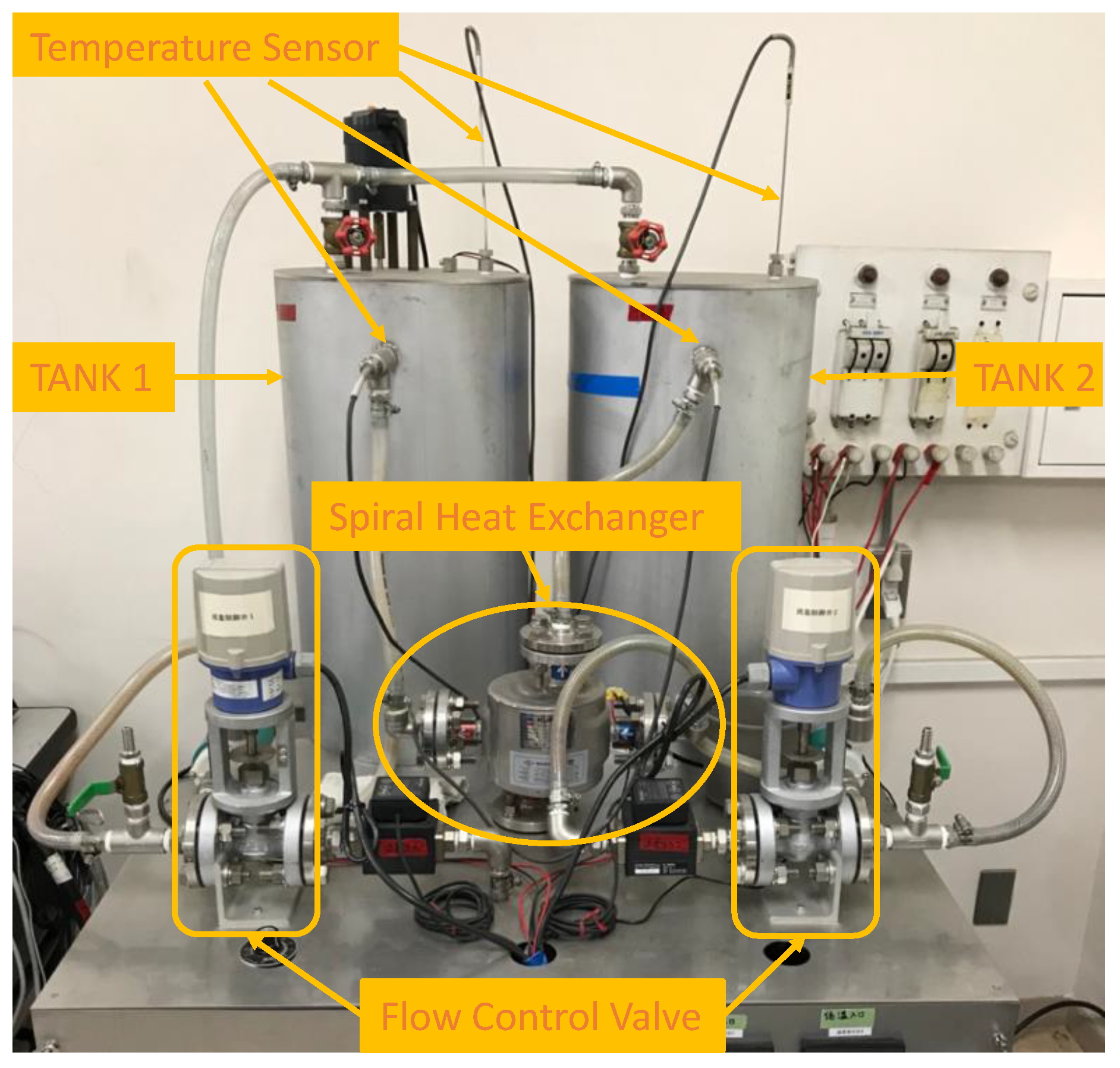
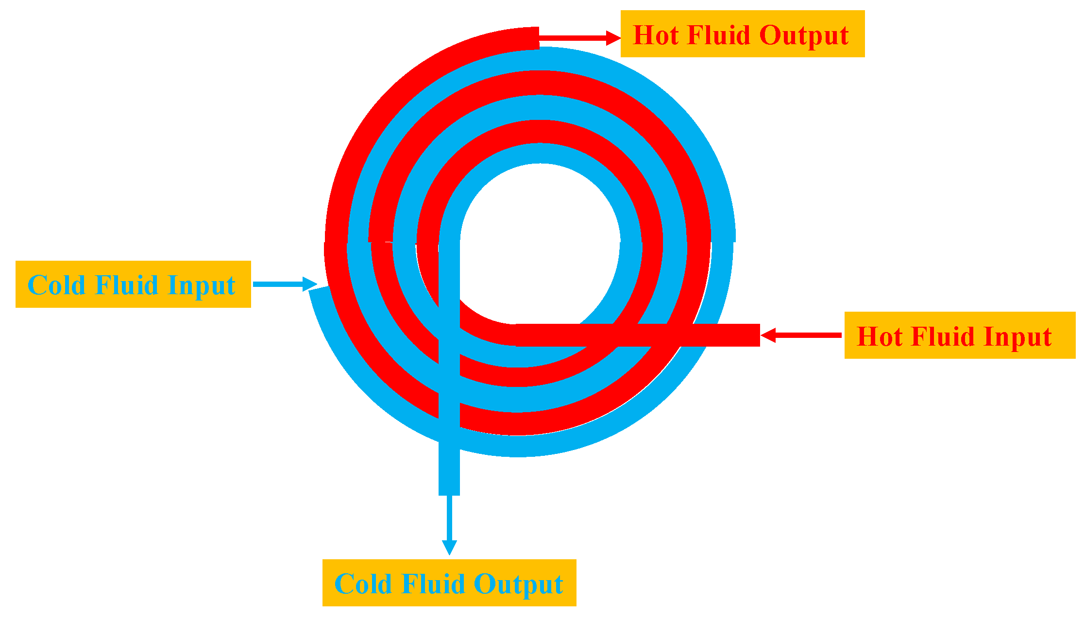
2.1. System Equipment and Modeling

The plant in this work is a heat exchange process with a spiral heat exchanger. For the details of the experimental equipment and system modeling of the plant, see Appendix A.

2.2. Generic Particle Filter

To overcome nonlinearity and non-Gaussianity, the particle filter is applicable to approximate the optimal Bayesian filter utilizing the important sequential Monte Carlo methodology. As a class of simulation filters, the particle filter recursively approximates the filtering random variable by ‘particles’ with discrete probability mass. In other words, a continuous variable is approximated by a discrete one with random support. These discrete points are viewed as samples. Particle filters treat the discrete support generated by the ‘particles’ as the true filtering density [28]. It performs filtering, namely, estimating the states (parameters or hidden variables) of a system, as a set of observations becomes available [29]. A complete representation of the posterior distribution of the states is allowed. Therefore, any nonlinearities or distributions can be dealt with using the particle filter. After state estimation, the observation value can be predicted based on the estimated state.

Consider the dynamic state space model of a statistical nonlinear system as follows:

$$\begin{array}{cc}\hfill x_t& =f\left(x_{t-1},u_{t-1},v_{t-1}\right)\hfill \\ \hfill y_t& =h\left(x_t,u_{t-1},n_t\right),\hfill \end{array}$$

(1)

where $f(·)$ is the process model that encodes the evolution of the state sequence, $h(·)$ is the measurement model associated with the state, $u_t$ is deterministic control input, while the process model noise sequence $v_t$ and measurement noise $n_t$ are independent and identically distributed and comply with any given distribution. The pdf of the initial state $p\left(x_0\right|y_0)\equiv p\left(x_0\right)$ is assumed to be available and subject to Gaussian distribution in this work.

According to Bayesian theory and the law of large numbers, a particle filter is designed for the estimation of the posterior distribution $p\left(x_t\right|y_{1:t})$ via N weighted samples $\{x_t^i,w_t^i\},i=1,\cdots ,N$, which are drawn from an importance proposal distribution $q(·)$. The weight for each sample can be calculated recursively as

$${\omega }_t^i={\omega }_t^{i-1}\frac{p\left(y_t\mid x_t^i\right)p\left(x_t^i\mid x_{t-1}^i\right)}{q\left(x_t^i\mid x_{t-1}^i,y_t\right)}.$$

(2)

Equation (2) shows the absolute particle weight, where $p\left(y_t\mid x_t^i\right)$ is likelihood and $p\left(x_t^i\mid x_{t-1}^i\right)$ is prior distribution. Theoretically, the importance proposal distribution $q(·)$ should be selected as similar as the posterior probability $p\left(x_t\right|y_t)$. However, the closed form of $p\left(x_t\right|y_t)$ is not able to be precisely approached. $q\left(x_t^i\mid x_{t-1}^i,y_t\right)=p\left(y_t\mid x_t^i\right)$ is selected as the importance proposal distribution in the filter design in this paper. In such a way, Equation (2) is simplified into

$${\omega }_t^i={\omega }_t^{i-1}p\left(y_t\mid x_t^i\right).$$

(3)

The estimated state ${\widehat{x}}_t$ can be approximated by the sum of N weighted samples

$${\widehat{x}}_t=\sum _{i=1}^N{\widehat{\omega }}_t^i{x}_t^i,$$

(4)

where ${\widehat{\omega }}_t^i$ is the normalized weight,

$${\widehat{\omega }}_t^i=\frac{{\omega }_t^i}{{\sum }_{i=1}^N{\omega }_t^i}.$$

(5)

After receiving the estimated state value, the measurement ${\widehat{y}}_t$ can be predicted by a substitution of the estimated value of state into the measurement model, as shown in Equation (6).

$${\widehat{y}}_t=h\left({\widehat{x}}_t,u_t\right)$$

(6)

The particle degeneracy phenomenon is common in a particle filter, where after a few iterations, all but one particle will have a negligible weight. A suitable measure of degeneracy is an estimation of the effective sample size $N_{eff}$ [30] defined as

$${\hat{N}}_{eff}=\frac{1}{{\sum }_{i=1}^N{\left({\widehat{\omega }}_t^i\right)}^2},$$

(7)

where small $N_{eff}$ indicates severe degeneracy. When $N_{eff}$ exceeds the threshold $N_{threshold}$, resampling will be performed. After resampling, the weight of each particle will become $1/N$.

2.3. Problem Statement

It must be mentioned that when the actual noise in a system is much higher than the noise modeled by the measurement model of a particle filter, the estimated value can no longer reflect the true state. In this paper, to deal with the fact that the particle filter algorithm cannot operate normally when encountering realistic large sensor noise and time delay, leading to the interruption of the entire control system incorporating the particle filter algorithm, exponential weight is employed as a weight adjustment to guarantee the continuous operation of the control system. Throughout this paper, the scale of the sensor noise is relative to the noise modeled by the measurement model in the particle filter algorithm.

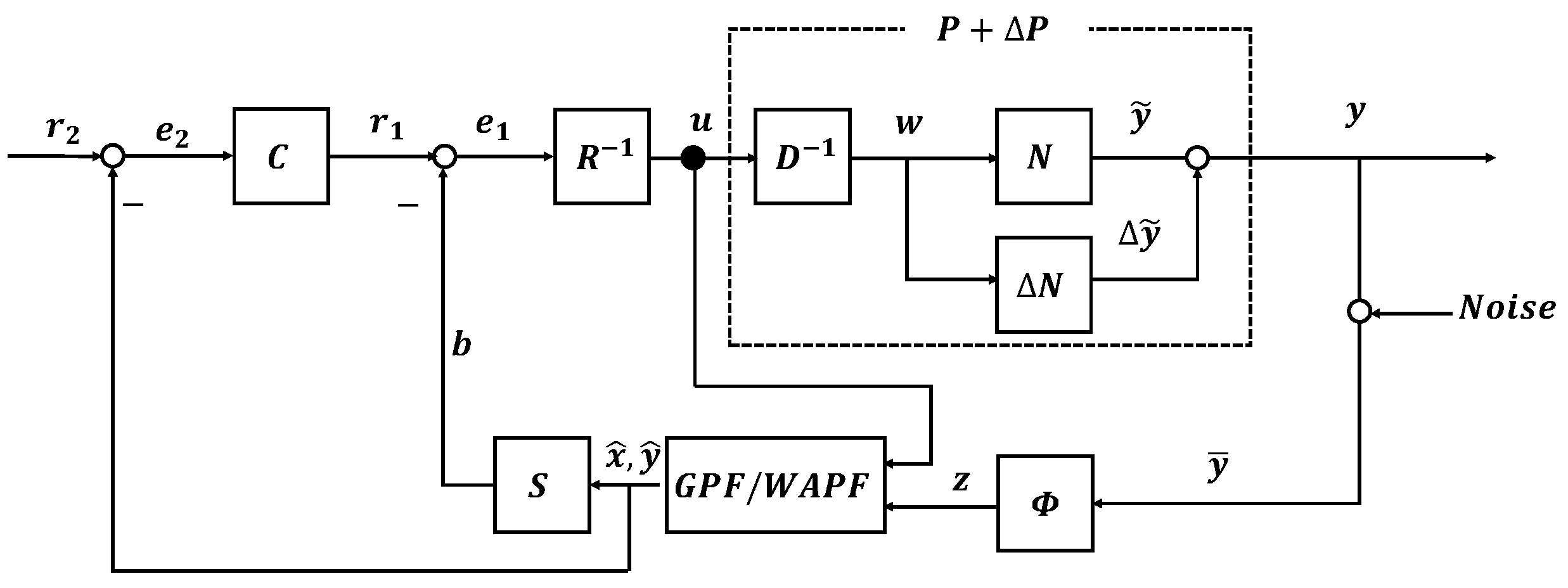
3. Particle Filter with Weight Adjustment Design for the Compensation of Sensor Noise and Time Delay

In this section, the uncertain heat exchange control system design using operator theory is first described. Then, the particle filter with the weight adjustment is designed to compensate for the influence of large sensor noise and time delay in wireless communication links. Moreover, the comparison of the two methods of exponential weights is discussed and the tracking performance is proved.

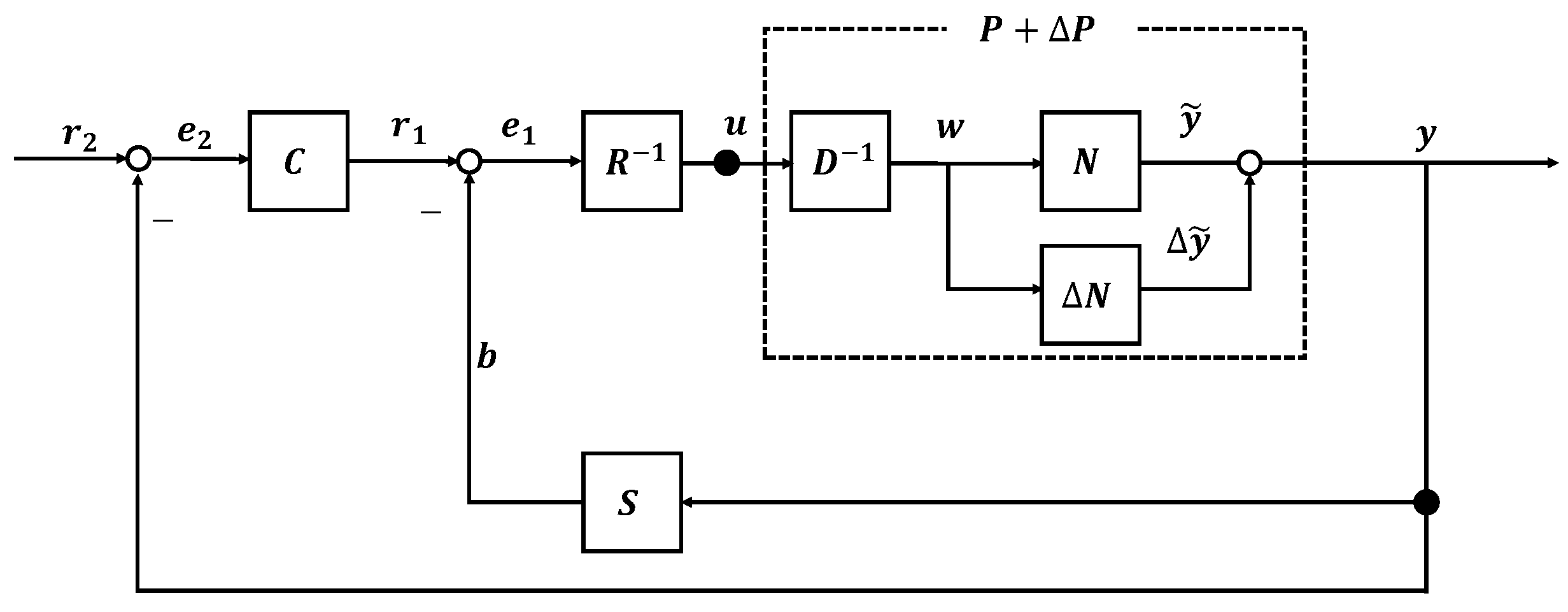
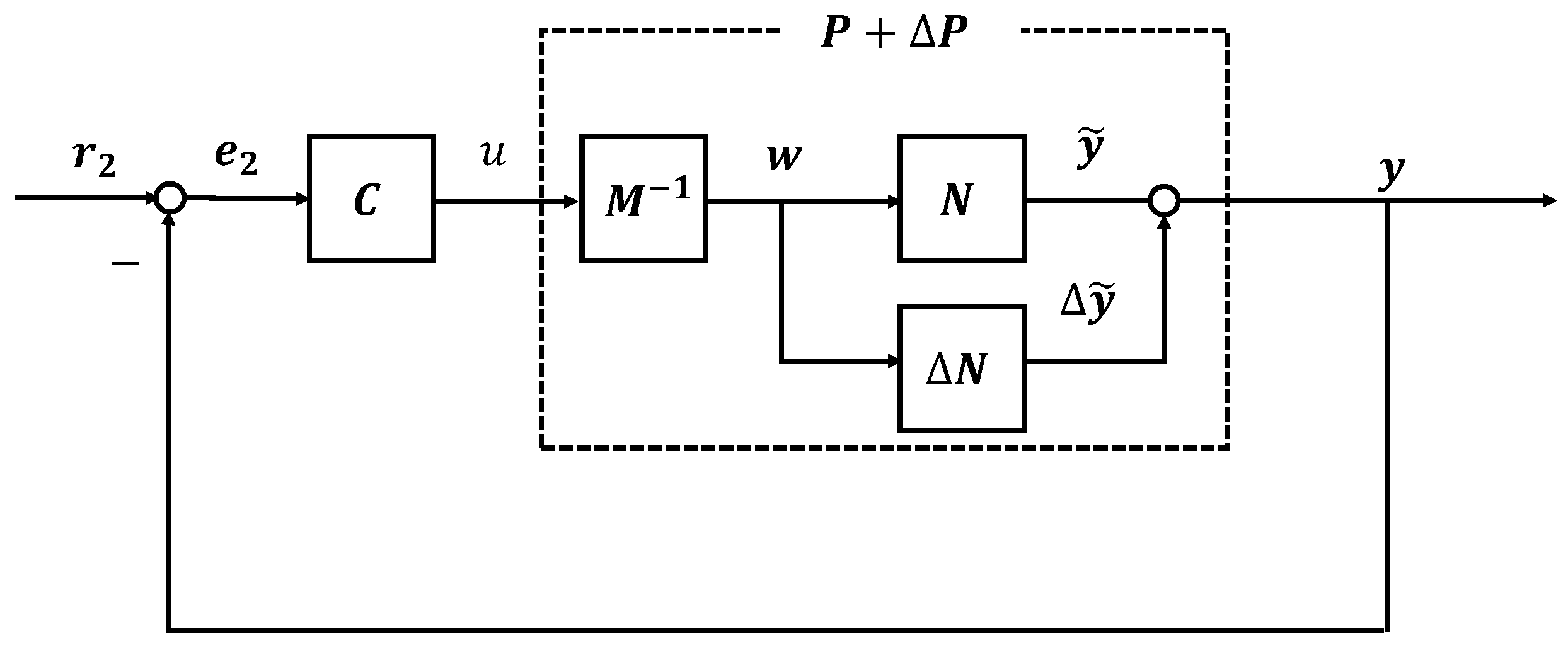
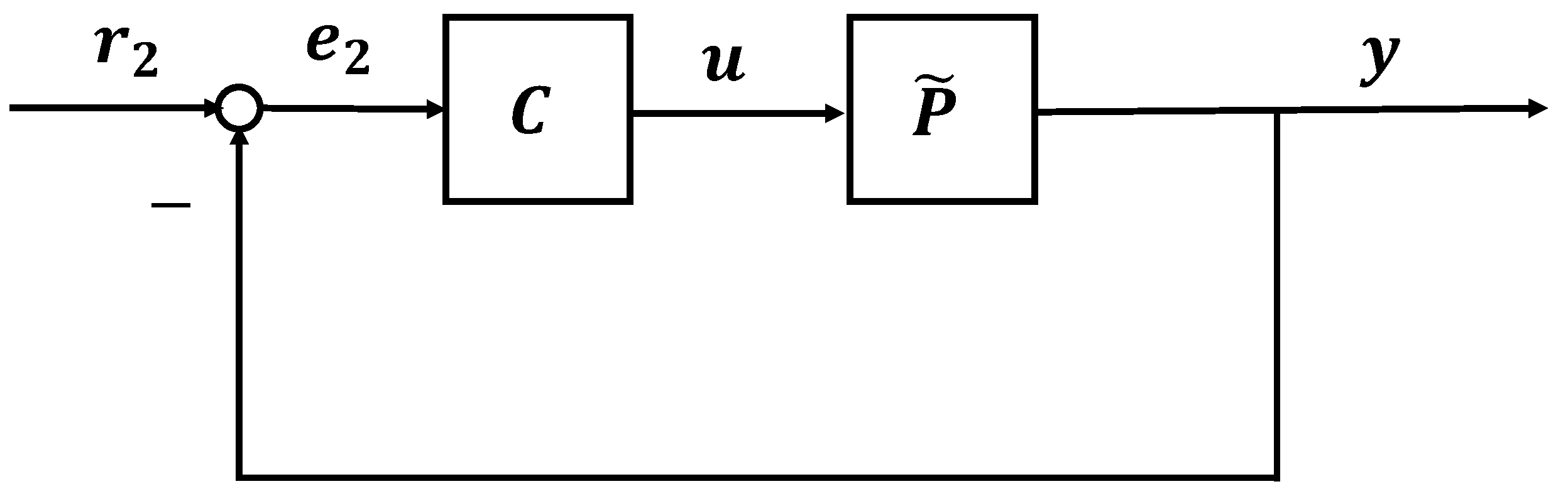
3.1. Operator Based Control System Design

Figure 1 shows the overall control system design scheme, which is based on operator theory, and its BIBO stability is ensured using Bézout identity, where $u\in U$, $y\in Y$, $w\in W$ are the input and output of the plant $P(U\to Y)$ and the output of a space change operator, respectively, and $r_2$ is the reference input. $P=N{D}^{-1}$ and $P+\Delta P=(N+\Delta N)D^{-1}$ are the nominal plant and uncertain plant with right factorization, respectively, where N is stable, D is stable and invertible, and $\Delta N$ is unknown. Based on Bézout identity in Equation (8), if Equation (9) holds, where M and $\tilde{M}$ are unimodular operators, then the nonlinear feedback control system with uncertainty is robust stable and the stabilizing operators S and R are designed as in Equation (10).

$$\begin{array}{c}SN+RD=M\end{array}$$

(8)

$$\begin{array}{c}\left\{\begin{array}{c}S(N+\Delta N)+RD=\tilde{M}\hfill \\ ∥(S(N+\Delta N)-AN){\tilde{M}}^{-1}∥<1\hfill \end{array}\right.\end{array}$$

(9)

$$\begin{array}{cc}\hfill & N:Y\to U\hfill \\ \hfill & b\left(t\right)=\frac{1-K}{\frac{A_1+A_5}{ln\left[\frac{T_{ho}\left(t\right)-T_{co}\left(t\right)}{T_{hi}-T_{ci}\left(t\right)}\right]-\frac{A_4}{t}ln\left[\frac{T_{hi}-T_{ci}\left(t\right)}{T_{hi}\left(0\right)-T_{ci}\left(0\right)}\right]}-A_3}\hfill \\ \hfill & R:U\to U\hfill \\ \hfill & e\left(t\right)=\frac{K}{A_2}u\left(t\right)\hfill \end{array}$$

(10)

where K is the design parameter, and 

$$\begin{array}{ccc}{A}_1=\frac{2a{\left(6\pi \right)}^3}{3\lambda }\hfill & A_2=-\frac{R_e{P}_{r}A}{N_{\mu }{c}_{\rho }\rho }\hfill & A_3=\frac{\delta }{\lambda }+\frac{1}{h_c}\hfill \\ A_4=\frac{a^2{\left(6\pi \right)}^4{c}_{\rho }\rho }{4\lambda }\hfill & A_5=\frac{a^2{\left(6\pi \right)}^4}{2d_r\lambda }\hfill \\ N_{\mu }=0.023R_e^{0.8}{P}_r^{0.3}\hfill & h_c=\frac{c_{\rho }\rho U_c{N}_{\mu }}{R_e{P}_{r}A}.\hfill \end{array}$$

(11)

where the parameters can be found in

Table 1. Parameters.

r	Target temperature value	35 °C
$T_{hi}$	Hot fluid outlet temperature	40 ${}^{\circ }$C
$T_{ci}\left(0\right)$	Initial cold fluid inlet temperature	26 ${}^{\circ }$C
$T_{co}\left(0\right)$	Initial cold fluid temperature	26 ${}^{\circ }$C
$U_{hmax}$	Max of hot fluid flow rate	5.4 L/min
$U_c$	Cold fluid flow rate	4.3 L/min
a	Archimedes’ spiral equation constant	$8\times {10}^{-7}$ m/rad
$\lambda$	Thermal conductivity of SUS304	16.7 W/(m·${}^{\circ }$C)
$R_e$	Reynolds number	22,000
$P_r$	Prandtl number	7
A	Cross-section area of flow path	$5.5\times {10}^{-4}$ m${}^2$
$c_{\rho }$	Specific heat of water	4.2 kJ/(kg·${}^{\circ }$C)
$\rho$	Density of water	1000 kg/m${}^3$
$\delta$	Thickness of heat exchanger’s wall	$1.83\times {10}^{-3}$ m
$dr$	Width of flow path	$5\times {10}^{-3}$ m
m	Mass of cold fluid flow rate	0.0717 kg
$\delta m$	Uncertainty of m	0.015 kg
M	Mass of cold fluid in TANK2	31.8 kg
$\alpha$	$T_{ci}$-$U_h$ Design parameter	0.3 L/min
$\beta$	$T_{ho}$-$U_h$ Design parameter	0.03
$\gamma$	Design parameter for valve of hot fluid	1.25
$\kappa$	Design parameter for flow change of hot fluid	0.026
K	Design parameter of $S,R$	0.7
$K_{\alpha }$	Proportional gain of C	2000
$K_{\beta }$	Integral gain of C	97
$\Delta t$	Sampling time	1 s
$T_{end}$	Simulation time	2401 s
$\sigma$	Standard deviation of likelihood function	0.01 ${}^{\circ }$C

.

The tracking controller C is

$$C\left(e_2\right)\left(t\right)=K_{\alpha }{e}_2\left(t\right)+K_{\beta }{\int }_0^t{e}_2\left(\tau \right)d\tau .$$

(12)

The above is the robust nonlinear uncertain heat exchange control system design that is not subject to sensor noise and wireless communication delay. Considering sensor noise and time delay, in order to not redesign the controller, the particle filter algorithm with a weight adjustment is incorporated into the system to estimate the state and predict the output from the measurement that is corrupted by sensor noise and time delay.

3.2. Particle Filter with Weight Adjustment Design to Compensate the Influence of Sensor Noise and Time Delay

Considering the sensor noise and time delay existing in the system output, the particle filter is put into an uncertain heat exchange control system for state estimation and further output prediction to avoid the reconfiguration of controller. The estimated states and the predicted output values calculated using the particle filter that have mitigated the influence of noise and time delay will be substituted for the corrupted output picked up from sensors and passed through wireless communication to be fed into the feedback loop. Figure 2 shows the particle filter with the weight adjustment design scheme of an uncertain heat exchange control system, where GPF is a generic particle filter, WAPF is the particle filter with the weight adjustment, $\mathsf{\Phi }$ is a time-varying time delay component due to the use of wireless communication, y is the system output and regarded as the measurement value that has not been affected by sensor noise and time delay, $\overline{y}$ is the output with a random noise and time delay, $\widehat{x}$ and $\widehat{y}$ are the states and output reconstructed by the particle filter from the impaired signal, which will then be conveyed to operator S as the feedback signal of the system. $\mathit{Noise}$ in this paper is additive Gaussian noise. Other components are defined in accordance with Figure 1.

In the component GPF/WAPF, controlled variables $T_{ci}\left(t\right)$ and $T_{ho}\left(t\right)$ are assumed as state variables $x_{T_{ci},t}$ and $x_{T_{ho},t}$, which will be estimated as the sum of weighted particles (corresponding to $\widehat{x}$ in Figure 2), manipulated variable $U_{h\left(t\right)}$ is $U_{h,t}$, and controlled variable $T_{co,t}$ is measurement variable $y_{T_{co,t}}$ which is predicted using Equation (6) (corresponding to $\widehat{y}$ in Figure 2). To formulate a paradigm for the particle filter, the process model is established as Equation (13),   

$$\begin{array}{cc}\hfill T_{ci}\left(t\right)& =\frac{m+\Delta m}{m+\Delta m+M}{T}_{co}(t-\Delta t)+\frac{M}{m+\Delta m+M}{T}_{ci}(t-\Delta t)\hfill \\ \hfill X\left(t\right)& =\frac{U_h\left(t\right)+\alpha }{U_h\left(t\right)+U_c}{T}_{hi}+\frac{U_c-\alpha }{U_h\left(t\right)+U_c}{T}_{ci}\left(t\right)\hfill \\ \hfill T_{ho}\left(t\right)& =(1-\beta )T_{ho}(t-\Delta t)+\beta X\left(t\right),\hfill \end{array}$$

(13)

and the measurement model is established as Equation (14),

$$\begin{array}{cc}\hfill Y\left(t\right)& =\frac{\gamma U_h\left(t\right)}{U_{hmax}}\hfill \\ \hfill Z\left(t\right)& =(1-\kappa )Z(t-\Delta t)+\kappa \dot{Y}\left(t\right)\hfill \\ \hfill T_{co}\left(t\right)& =T_{ci}\left(t\right)+\left[T_{hi}-T_{ho}\left(t\right)\right]Z\left(t\right),\hfill \end{array}$$

(14)

where the process noise and measurement noise comply with Gaussian distribution. For the physical meaning and values in the equations, please refer to Appendix A and Table 1.

It can be noticed that in the first equation of the state transition model shown in Equation (13), the calculation of $x_{T_{ci},t}$ consists of the information of measurement value $y_{T_{co},t-1}$, which seems not to meet the Markovian assumption in the particle filter. However, in a generic particle filter, the prior distribution is by far the most popular importance density in the literature [25], and such importance density is also adopted in this paper, as illustrated in Section 2.2. In such a way, the posterior probability modification effect on particle sampling is ignored. Inspired by the motivation of the auxiliary variable particle filter [28], where the most promising particles (high prediction likelihood) at time $t-1$ are expanded to time t, thereby merging the information of posterior probability to generate sampled particles, the posterior information at the previous time instant $y_{T_{co},t-1}$ is integrated into the particle sampling procedure at time t. Furthermore, the influence of the posterior information at time $t-1$ on the sampled particles is applied with an appropriate proportion. In this work, the proportion is set as $(m+\Delta m)/(m+\Delta m+M)$, which is exactly in line with the physical laws of reality.

Taking the time delay element into account yields

$$z_t=\mathsf{\Phi }\left({\overline{y}}_t\right)=\overline{y}(t-d),$$

(15)

where d represents the time delay. Please refer to [14] for the method of generating the time delay. If the sensor noise (denoted here as m) is put into the expression of the output from sensors and flowing through the wireless path, then the signal received by the particle filter is

$$z_t=(y+m)(t-d),$$

(16)

which is exactly the expression of the two interference items in the signal input to the particle filter algorithm. The particle filter is adopted for processing the signal subject to noise and time delay to acquire the approximation of system states and further the system output that reduced the impact of the above two factors. The residuals between the time-delayed output due to the wireless communication and undelayed particles contribute to the particle weight update. Therefore, the processing of the measurement values with noise and time delay is consistent with that of the general particle filter. That is, the two interference items are dealt with comprehensively in this work.

During the control process incorporated with a generic particle filter, it is found that large noise appearing in the measurement makes the posterior calculation less accurate. It is because measurements that are realistic given the high amount of noise obtain very low likelihoods, the measurement model judges such amounts of noise as highly unlikely, and the associated particles will be removed during the resampling step [21]. In detail, the prediction pdf of each particle is updated based on the residual $\left|re{s}_t^i\right|$ shown in Equation (17). Higher residuals result in a lower likelihood, meaning that the sampled particle is less likely to represent the true state and vice versa under the situation where the measurement is not polluted by actual large noise. However, when the actual measurement noise is much larger than the noise modeled in the measurement model of the particle filter, the residual will also become larger, resulting in a small particle weight. This will cause the state estimation in a generic particle filter to be no longer applicable, and the traditional resampling method to be meaningless. More extreme, if almost all particle weights are becoming smaller to a certain extent, system control incorporated with a particle filter cannot proceed normally, which will be shown in the simulation in Section 4.

$$\left|re{s}_t^i\right|=|{\overline{y}}_t-x_t^i|$$

(17)

For coping with the unsuitable particle weights for state estimation and subsequent resampling owing to the actual given large noise, it is a reasonable consideration to adopt a particle weight adjustment scheme. Precisely, when the realistic given system output ${\overline{y}}_t$ measured by sensors and transmitted through the wireless communication path is available, the residual $\left|re{s}_t^i\right|$, which represents the difference between the actual measurement and sampled particles, is first calculated and the $3\sigma$ rule is exploited to determine whether $\left|re{s}_t^i\right|$ is large so that the particle weight is pushed to a low likelihood. A small particle weight may indicate that the current measurement is affected by realistic large noises, but this judgment from only one particle is not absolutely accurate. When the number of particles that violate the $3\sigma$ rule reaches a certain proportion $prop$ of the total particles, it can be considered that the actual large noise has likely affected the current measurement adversely. At this time, exponential weights ${\omega }_{exp,t}^i$, taking the place of the original absolute weights $w_t^i$ at low likelihood due to large noise, are assigned to those particles outside the $3\sigma$ range. For particles within the $3\sigma$ range, the particle weights remain as the original absolute weights. Overall, particle weights are calculated with Equation (18). After that, the exponential weights and absolute weights are normalized to $[0,1]$ in Equation (19) for the subsequent state estimation and measurement prediction.

$$\begin{array}{c}{\tilde{\omega }}_t^i=\left\{\begin{array}{cc}{\omega }_{exp,t}^i=exp\left(w_t^i\right)\hfill & \mid {res}_t^i\mid >3\sigma \hfill \\ w_t^i\hfill & \mid {res}_t^i\mid \le 3\sigma \hfill \end{array}\right.\end{array}$$

(18)

$$\begin{array}{c}{\widehat{\omega }}_t^i=\frac{{\tilde{\omega }}_t^i}{{\sum }_{i=1}^N{\tilde{\omega }}_t^i}\end{array}$$

(19)

In summary, the particle filter with weight adjustment algorithm is shown in Algorithm 1.

3.3. Comparison of Two Methods of Exponential Weight

This work is inspired by the knowledge of information theory about information entropy and based on the consideration that when the realistic measurement is mixed with large noise, some particles that are likely to represent the true state may be removed from the generic particle filter. Information entropy represents the degree of uncertainty, and the largest entropy means the largest degree of uncertainty in the system. Among all possible probabilistic models (distributions), the model with the largest entropy is the best model. When the uncertainty in the system is the largest, that is, when any information in the system is unknown, no assumption is made about any unknown information, and the unknown information is treated with an equal probability.

Considering a dataset $T=\{(x_1,y_1),\cdots ,(x_n,y_n)\}$, where $x_i$ represents the value of the ith sample. At this time, the maximum entropy model is

$$P(y_i=k|x_i)=\frac{exp\left(w_k{x}_i\right)}{{\sum }_{k=1}^{K}exp\left(w_k{x}_i\right)},$$

(20)

where k represents the kth category, $y_i$ represents the label value of the ith sample, and $w_k$ represents the parameter corresponding to the kth category, indicating the probability that the ith sample belongs to the kth category. This is usually used for multi-classification problems. Putting it into the particle filter algorithm, it can be considered as that if the measurement affected by large noise is available, then the posterior distribution with the largest entropy is the best model, that is, to seek the sampling particles that are most likely to represent the real state. Corresponding to the above dataset, the problem to find the best posterior distribution can be illustrated as follows.

Algorithm 1 Particle filter with weight adjustment.

Input: ${\{x_{t-1}^i,{\widehat{\omega }}_{t-1}^i\}}_{i=1}^N,y_t$ Output:${\{x_t^i,{\widehat{\omega }}_t^i\}}_{i=1}^N$ Generate the initial N particles $x_0^i$ from its distribution, and set its weight as ${\widehat{\omega }}_0^i=1/N$  Loop process:  while $t\ge 1$ do      Set the normalization sum as ${\omega }_{sum}=0$      for $i=1,\cdots N$ do          draw samples from $x_t^i\sim q\left(x_t^i\right|x_{t-1}^i,y_t)$          assign weight ${\omega }_t^i$ according to Equation (3) and calculate $\left|re{s}_t^i\right|$, record the number $nu{m}_t$             of particles outside $3\sigma$ range            end for       Particle weight adjustment:      if $nu{m}_t>prop\ast N$ then          for $i=1,\cdots N$ do              if $\left|re{s}_t^i\right|>3\sigma$ then                   ${\tilde{\omega }}_t^i=exp\left({\omega }_t^i\right)$              else                   ${\tilde{\omega }}_t^i={\omega }_t^i$                 end if              Accumulate the normalization sum as ${\omega }_{sum}={\omega }_{sum}+{\tilde{\omega }}_t^i$           end for      end if      Normalize exponential weights and absolute weights Comprehensively:      for $i=1,\cdots N$ do          ${\widehat{\omega }}_t^i={\tilde{\omega }}_t^i/{\omega }_{sum}$      end for      State estimation and output prediction:      Estimate state according to Equation (4), and predict output according to Equations (6) and (14)      Resample particles:      if ${\widehat{N}}_{eff}<N_{threshold}$ then          Resample N particles with replacement          for $i=1,\cdots N$ do             ${\omega }_t^i=1/N$          end for      end if end while

At the current time t, regard $T=\{(y_t,x_t^1),(y_t,x_t^2),\cdots ,(y_t,x_t^N)\}$ as a dataset, where $x_t^i$ is the sampled particles at time t, and $y_t$ is the measurement at current time. Since the measurement is the only determined one, it can be seen as a correspondance of $x_i=1$ in Equation (20), so the value of $y_t$ in Equation (21) can be set as $y_t=1$. The number of categories K is the number of sampled particles N. The parameter $w_k$ corresponds to the particle weight ${\omega }_t^i$. Therefore, the posterior probability of having the maximum entropy at the current time can be expressed as the normalized exponential weight shown in Equation (21)

$$P\left(x_t^i\right|y_t)=\frac{exp\left({\omega }_t^i{y}_t\right)}{{\sum }_{i=1}^{N}exp\left({\omega }_t^i{y}_t\right)}=\frac{exp\left({\omega }_t^i\right)}{{\sum }_{i=1}^{N}exp\left({\omega }_t^i\right)}.$$

(21)

This is different from the described method in Section 3.2 and Algorithm 1. Through analysis, it can be found that this method has high requirements for the quality of sampled particles. If the sampled particles are very close to the real state, the estimated state will be very close to the real value. In other words, this method puts almost all trust in the sampled particles and relies heavily on the quality of sampled particles. If the quality of the sampled particles is not good enough, the estimated state value will deviate significantly from the true value. Multiple rounds of trial and error selection may be required to obtain a good state estimation. Moreover, this method will greatly suppress the effect of small-likelihood particles and maximize that of large-likelihood particles; therefore, it is likely that only several particles have large weights, while other particles have small weights, i.e., the particle degeneracy arises. Therefore, it is necessary to be modified.

In the modified method shown in Section 3.2 and Algorithm 1, only those particles outside the $3\sigma$ range are assigned with exponential weights, while the weights of other particles remain the absolute weights. Exponential weights retain the role of small weighted particles so that they can still play a role in state estimation. Furthermore, the concern of retaining the absolute weights for particles that do not violate the $3\sigma$ rule is that the current small weight might not be due to the measurement affected by actual large noise but sampling in the state prediction stage. The comprehensive consideration of the exponential weight and absolute weight is a relatively conservative strategy where both the realistic large noise and particle sampling are taken into account as the cause of the small weight, which is reasonable on account of the previous analysis. In addition, if all the weights are extremely small, it can be concluded that the measurement at this time is indeed adversely affected by large noise. The measurement mixed with large noise is unreliable, where all particles become nearly the same weight after the weight adjustment, and it is wise to treat all the sampled particles equally, as shown in Equation (22).

$$\begin{array}{cc}\hfill \underset{w_t^i\to 0}{lim}{\widehat{\omega }}_t^i& =\underset{w_t^i\to 0}{lim}\frac{{\tilde{\omega }}_t^i}{{\sum }_{i=1}^N{\tilde{\omega }}_t^i}\hfill \\ \hfill & =\underset{w_t^i\to 0}{lim}\frac{{\omega }_{exp,t}^i}{{\sum }_i^N{\omega }_{exp,t}^i}\hfill \\ \hfill & =\underset{w_t^i\to 0}{lim}\frac{exp\left(w_t^i\right)}{{\sum }_{i=1}^{N}exp\left(w_t^i\right)}\hfill \\ \hfill & =\frac{1}{N}\hfill \end{array}$$

(22)

3.4. Tracking Performance of the Particle Filter Design in Overall Control System

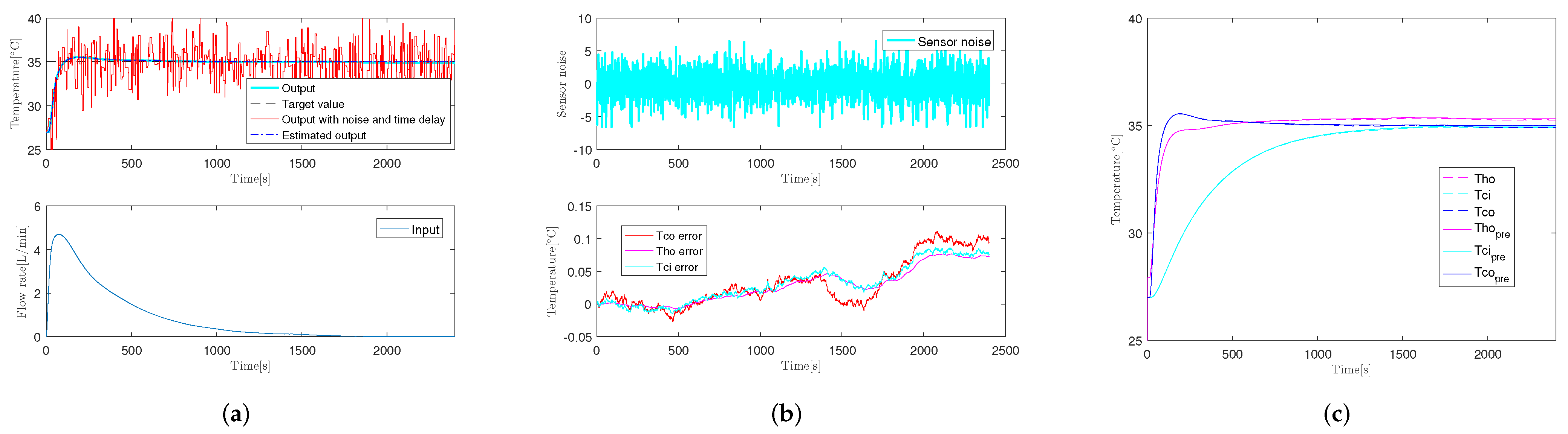
It should be noted that the control system design incorporating the particle filter with weight adjustment can still guarantee its tracking performance using the tracking controller described in Section 3.1, which illustrates that the incorporation of the particle filter avoids redesigning the controller.

Proof. 

Tracking performance using controller C.

Figure 2 can be re-expressed as Figure 3, where the uncertainty caused by state estimation and measurement prediction using particle filter and the structural uncertainty are summarized into $\Delta N$. Figure 4 shows the equivalent block-diagram of stabilizing system $\tilde{P}$.

From Figure 4, the error $e_2$ can be written as

$$e_2\left(t\right)={(I+\tilde{P}C)}^{-1}\left(r_2\right)\left(t\right),$$

(23)

where I is identity operator. From the exponential iteration theorem, ${(I+\tilde{P}C)}^{-1}\left(r_2\right)\left(t\right)$ exists [26]. Furthermore, we have [31]

$$\begin{array}{cc}\hfill y\left(t\right)& =r_2\left(t\right)-e_2\left(t\right)\hfill \\ \hfill & =r_2\left(t\right)-{(I+\tilde{P}C)}^{-1}\left(r_2\left(t\right)\right)\hfill \\ \hfill & =r_2\left(t\right)-{\left(r_2\left(t\right)+\tilde{P}C\left(r_2\left(t\right)\right)\right)}^{-1}\hfill \\ \hfill & =r_2\left(t\right)-{\left(r_2\left(t\right)+K_{\alpha }\tilde{P}\left(r_2\left(t\right)\right)+K_{\beta }{\int }_0^t\tilde{P}\left(r\left(\tau \right)\right)d\tau \right)}^{-1}.\hfill \end{array}$$

(24)

Considering the first condition that $\tilde{P}$ satisfies, as stated in [26], it is assumed that for all t in $[0,T]$, C is stable and $\tilde{P}\left(u\right)\ge K_l$ as $T\ge t{\ge }_1\ge 0$, $u>0$, then

$$\begin{array}{cc}\hfill & K_{\alpha }\tilde{P}\left(r_2\left(t\right)\right)+K_{\beta }{\int }_0^t\tilde{P}\left(r\left(\tau \right)\right)d\tau \hfill \\ \hfill & \ge K_{\alpha }{K}_l+K_{\beta }{\int }_0^t\tilde{P}\left(r_2\left(\tau \right)\right)\hfill \\ \hfill & \ge K_{\alpha }{K}_l+K_{\beta }{\int }_0^{t_1}\tilde{P}\left(r\left({\tau }_1\right)\right)d{\tau }_1+K_{\beta }{K}_l{\int }_{t_1}^{t}d{\tau }_2.\hfill \end{array}$$

(25)

$K_{\beta }{K}_l{\int }_{t_1}^{t}d{\tau }_2$ can be made arbitrarily large by making $t<T$ large enough and selecting an appropriate $K_l$, then ${\left(r_2\left(t\right)+K_{\alpha }\tilde{P}\left(r_2\left(t\right)\right)+K_{\beta }{\int }_0^t\tilde{P}\left(r\left(\tau \right)\right)d\tau \right)}^{-1}$ can be made arbitrarily small, indicating that $y\left(t\right)-r_2\left(t\right)$ can be made arbitrarily small, so $y\left(t\right)$ can track $r_2\left(t\right)$. □

4. Simulation

In this section, the simulation results of the particle filter with weight adjustment design for the robust nonlinear uncertain heat exchange process in Figure 2 will be given to demonstrate the effectiveness of the method. The simulation time is set as 2401 s, the sampling time is set as $\Delta t=1$ s, the parameter values used are listed in Table 1, the number of particles is $N=200$, and the time delay is assumed to be subject to Gaussian distribution. Because the effect of time delay on the control system has been verified in [14], it will not be repeated, and the effect of sensor noise and time delay will be shown comprehensively here. In the simulation, the method of generating the time delay and its distribution remain unchanged, and only the variance of sensor noise is changed to obtain sensor noise of different scales relative to that modeled in the measurement model in the particle filter. The following set of equations are considered an illustrative example:

$$\begin{array}{cc}\hfill p\left(x_t\mid x_{t-1}\right)& =\mathcal{N}\left(x_t;f\left(x_{t-1},u_t\right),{\sigma }_v^2\right)\hfill \\ \hfill p\left(y_t\mid x_t\right)& =\mathcal{N}\left(y_t;h\left(x_t,u_t\right),{\sigma }_n^2\right)\hfill \\ \hfill p\left(n_s\right)& =\mathcal{N}\left({\mu }_s,{\sigma }_s^2\right),\hfill \end{array}$$

(26)

where ${\sigma }_v^2$ and ${\sigma }_n^2$ are variances of process noise and measurement noise modeled in the particle filter, respectively, and ${\sigma }_v^2=0.{001}^2$ and ${\sigma }_n^2=0.1^2$. $f(·)$ and $h(·)$ are the process model and measurement model without noise and the same as in Equation (1). ${\mu }_s$ and ${\sigma }_s^2$ are the mean and variance of sensor noise, and ${\mu }_s=0$ and ${\sigma }_s^2$ is set as different values. The mean of process noise and measurement noise modeled in the particle filter is 0.

Figure 5 shows the result under sensor noise (${\sigma }_s^2=0.3^2$) and time delay without particle filter, where Figure 5a shows the system output $T_{co}$, the target value $r_2$ and the output affected by sensor noise and time delay, Figure 5b shows the sensor noise imposed on the output. The system states $T_{ho}$, $T_{hi}$ and system output $T_{co}$ are also shown in Figure 5b, where since the value of hot fluid input $T_{hi}$ is a constant, it is not displayed. It can be observed that the control performance is not satisfactory due to sensor noise and time delay. There is an oscillation in both output and input values, and there is even a tendency to deviate from the target value after about 1550 s.

Figure 6 shows the result using a generic particle filter to reduce the effect of noise and time delay with the same noise variance as in Figure 5. It is clear that the particle filter does improve the control performance under noise and time delay. Figure 6a shows the output and input results as illustrated in Figure 5a, and it can be seen that the stability and the tracking performance can be guaranteed. Figure 6b shows the sensor noise imposed on the system output, the error between states estimated using GPF and that from the system ($T_{ho}$ error and $T_{ci}$ error), and the error between output predicted using GPF and that from the system ($T_{co}$ error). From Figure 6b, the variance of the error between the states output from GPF and that from the system has been reduced compared with the given sensor noise, which demonstrates that the influence of sensor noise has decreased. Figure 6c shows the states and output constructed from particle filter and that from the system, which is not imposed sensor noise and time delay, where the states and output using GPF is very close to that of the system.

Figure 7 and Figure 8 display the results when sensor noise is increased, where variance grows from ${\sigma }_s^2=0.3^2$ to ${\sigma }_s^2=0.7^2$, and further increased relative to the measurement noise modeled in the particle filter. The system can guarantee the stability and tracking performance with the incorporation of a generic particle filter, as shown in Figure 8, while divergence occurs in the system after about 1000 s without a particle filter, as shown in Figure 7. Compared with the results with and without a particle filter, it is clear that a particle filter does reduce the effect of sensor noise and time delay on the control performance.

However, when the sensor noise becomes larger to a certain extent (${\sigma }_s^2=1.5^2$) relative to the measurement noise modeled in the particle filter (${\sigma }_n^2=0.1^2$), the generic particle filter cannot work normally. According to the analysis in Section 3.2 and Section 3.3, this is because the measurement noise pushes nearly all the sampled particles to low likelihoods, which will be removed in resampling and cause particle degeneracy. The particle weights can become extremely small, even exceeding the limit of storage under the reality that the amount of calculation storage is limited; thus, the state cannot be estimated and the particle filter algorithm collapses, which drags the system down to discontinuity, as shown in Figure 9. Note that because the noise is generated independently of the control system, it is not consistent with the states, the input and output of the control system in terms of time, as in Figure 9b.

Particle weight is adjusted according to Algorithm 1. The proportion of particles that violate the $3\sigma$ rule to judge if weight adjustment needs to be employed is set as $prop=70\%$. Figure 10 shows the effectiveness of the weight adjusted particle filter in the reduction in the large noise impact. It is clear that after adopting the particle filter with weight adjustment algorithm, the continuous operation, stability and tracking performance of the system are all guaranteed.

Figure 11 shows that when the variance of sensor noise grows (${\sigma }_s^2=1.7^2$), due to the influence of large sensor noise, the generic particle filter algorithm loses its function and the operation is interrupted, then the whole system is implicated.

In contrast, when the particle filter with weight adjustment algorithm is employed, the stable and continuous operation of not only the particle filter algorithm itself but also the entire system can be achieved, as shown in Figure 12.

In order to further illustrate the effectiveness and usefulness of the method, Figure 13 and Figure 14 show the simulation results of the particle filter with weight adjustment for mitigating the noise impact on system continuity, stability, and tracking performance when the noise further increases. In these cases, the particle filter with weight adjustment algorithm can still work normally even when the sensor noise largely increases relative to the modeled one. Further, the stability and tracking performance of the overall control system incorporated with particle filter with weight adjustment is guaranteed.

From the above simulation results, the generic particle filter and particle filter with weight adjustment design scheme indeed reduce the influence of sensor noise and time delay so that the continuity, stability, and tracking performance of the system can be guaranteed with no need to redesign the controller. In order to quantitatively illustrate the validity of the method, the variance is listed in

Table 2. Sensor noise reduction under different simulation cases.

Figure	GPF/WAPF	$\mathit{var}(\mathit{sn}.\mathit{set})$	$\mathit{var}(\mathit{sn}.\mathit{sim})$	$\mathit{var}\left({\mathit{E}}_{{\mathit{T}}_{\mathbf{ci}}}\right)$	$\mathit{var}\left({\mathit{E}}_{{\mathit{T}}_{\mathbf{ho}}}\right)$	$\mathit{var}\left({\mathit{E}}_{{\mathit{T}}_{\mathbf{co}}}\right)$
Figure 6	1/0	$0.3^2$	$0.0899$	$1.08\times {10}^{-4}$	$0.26\times {10}^{-5}$	$3.62\times {10}^{-4}$
Figure 8	1/0	$0.7^2$	$0.483$	$2.27\times {10}^{-4}$	$1.37\times {10}^{-4}$	$3.77\times {10}^{-4}$
Figure 9	1/0	$1.5^2$	$2.29$	$NaN$	$NaN$	$NaN$
Figure 10	0/1	$1.5^2$	$2.377$	$3.20\times {10}^{-4}$	$1.91\times {10}^{-4}$	$3.65\times {10}^{-4}$
Figure 11	0/1	$1.7^2$	$3.053$	$NaN$	$NaN$	$NaN$
Figure 12	0/1	$1.7^2$	$2.923$	$3.78\times {10}^{-4}$	$2.84\times {10}^{-4}$	$5.59\times {10}^{-4}$
Figure 13	0/1	$1.9^2$	$3.891$	$1.35\times {10}^{-4}$	$6.74\times {10}^{-5}$	$1.38\times {10}^{-4}$
Figure 14	0/1	$2.0^2$	$4.104$	$1.47\times {10}^{-4}$	$1.10\times {10}^{-4}$	$2.60\times {10}^{-4}$

, where GPF and WAPF represent the generic particle filter and particle filter with weight adjustment algorithm, respectively. As described above, 1 means that the method is used and 0 means that the method is not used, $var(sn.set)$ represents the variance of the sensor noise set in simulation, $var(sn.sim)$ represents the variance of the actual displayed sensor noise in simulation, and $var\left(E_{T_{ci}}\right)$ represents the variance of state $T_{ci}$ error, which is the difference between the state value estimated by the particle filter and that from the system. Similarly, $var\left(E_{T_{ho}}\right)$ represents the state $T_{ho}$ error, and $var\left(E_{T_{co}}\right)$ represents the variance of the output $T_{co}$ error, which is the difference between the output value predicted by particle filter and that of the system without noise and time delay. It can be seen from Table 2 that after incorporating the generic particle filter algorithm into the control system, the variance of the sensor noise is reduced when the variance of sensor noise imposed is ${\sigma }_s^2<1.5^2$. However, as the sensor noise increases to ${\sigma }_s^2\ge 1.5^2$ (about ${15}^2$ times the modeled noise), the particle filter with weight adjustment algorithm is necessary and the incorporation of that is effective in reducing the effects of large sensor noise.

5. Conclusions

In this paper, concerning the influence of sensor noise and wireless communication time delay on the robust nonlinear uncertain heat exchange control system, a particle filter is incorporated into the overall control system to deal with the adverse effect of the above two factors so as to avoid the reconfiguration of the controller. Considering that when encountering large sensor noise, the incorporated particle filter algorithm cannot operate normally, which leads to the interruption of the control system, inspired by the information theory knowledge about the principle of maximum entropy, the calculation method of particle weights is modified, where the exponential particle weights are substituted for the original absolute particle weights when the number of particles that violate the $3\sigma$ rule arrives at the set proportion and residual exceeds the $3\sigma$ range. The simulation verifies the validity of the weight adjustment in the particle filter for large noise and time delay simultaneously.

Sensor noise and time delay are considered and dealt with comprehensively in this work. In future work, sensor noise and time delay can be processed separately, where a better control performance could be expected. Moreover, H-infinity filtering [32] and Luenberger observers [33] are good estimation methods, and these methods can be employed in the future work.

References

1. Lee, M.-T.; Chuang, M.-L.; Kuo, S.-T.; Chen, Y.-R. UAV Swarm Real-Time Rerouting by Edge Computing D* Lite Algorithm. Appl. Sci. 2022, 12, 1056. [Google Scholar] [CrossRef]
2. Tseng, Y.-F.; Gao, S.-J. Decentralized Inner-Product Encryption with Constant-Size Ciphertext. Appl. Sci. 2022, 12, 636. [Google Scholar] [CrossRef]
3. Lounasmaa, O.V.; Seppä, H. SQUIDs in neuro-and cardiomagnetism. J. Low Temp. Phys. 2004, 135, 295–335. [Google Scholar] [CrossRef]
4. Tipsuwan, Y.; Chow, M.Y. Control methodologies in networked control systems. Control Eng. Pract. 2003, 11, 1099–1111. [Google Scholar] [CrossRef]
5. Otanez, P.G.; Moyne, J.R.; Tilbury, D.M. Using deadbands to reduce communication in networked control systems. In Proceedings of the 2002 American Control Conference, Anchorage, AK, USA, 8–10 May 2002. [Google Scholar]
6. Jiang, L.; Deng, M.; Inoue, A. Obstacle avoidance and motion control of a two wheeled mobile robot using SVR technique. Int. J. Innov. Comput. Inf. Control 2009, 5, 253–262. [Google Scholar]
7. Deng, M.; Kawashima, T. Adaptive Nonlinear Sensorless Control for an Uncertain Miniature Pneumatic Curling Rubber Actuator Using Passivity and Robust Right Coprime Factorization. IEEE Trans. Control Syst. Tech. 2016, 24, 318–324. [Google Scholar] [CrossRef]
8. Deng, M.; Saijo, N.; Gomi, H.; Inoue, A. A robust real time method for estimating human multijoint arm viscoelasticity. Int. J. Innov. Comput. Inf. Control 2006, 2, 705–721. [Google Scholar]
9. Deng, M.; Inoue, A.; Zhu, Q. An integrated study procedure on real time estimation of time varying multijoint human arm viscoelasticity. Trans. Inst. Meas. Control 2011, 33, 919–941. [Google Scholar] [CrossRef]
10. Pugalenthi, K.; Trung Duong, P.L.; Doh, J.; Hussain, S.; Jhon, M.H.; Raghavan, N. Online Prognosis of Bimodal Crack Evolution for Fatigue Life Prediction of Composite Laminates Using Particle Filters. Appl. Sci. 2021, 11, 6046. [Google Scholar] [CrossRef]
11. Wigren, A.; Wågberg, J.; Lindsten, F.; Adrian, G.W.; Thomas, B.S. Nonlinear System Identification: Learning While Respecting Physical Models Using a Sequential Monte Carlo Method. IEEE Control Syst. Mag. 2022, 42, 75–102. [Google Scholar] [CrossRef]
12. Naesseth, C.; Linderman, S.; Ranganath, R.; Blei, D. Variational sequential Monte Carlo. Proc. Mach. Learn. Res. 2018, 84, 968–977. [Google Scholar]
13. Han, X.; Wu, B.; Wang, D. Firefly algorithm with disturbance-factorbased particle filter for seismic random noise attenuation. IEEE Trans. Geosci. Remote Sens. 2019, 17, 1268–1272. [Google Scholar] [CrossRef]
14. Naka, H.; Deng, M.; Noge, Y. Experimental Research on Nonlinear Process Output Estimation System by DCS Devices. In Proceedings of the International Conference on Advanced Mechatronic Systems, Shiga, Japan, 26–28 August 2019. [Google Scholar]
15. Martino, L.; Read, J.; Elvira, V.; Louzada, F. Cooperative parallel particle filters for online model selection and applications to urban mobility. Digit. Signal Process. 2017, 60, 172–185. [Google Scholar] [CrossRef] [Green Version]
16. Doucet, A.; Johansen, A.M. A tutorial on particle filtering and smoothing: Fifteen years later. In Handbook of Nonlinear Filtering; Oxford University Press: Oxford, UK, 2009. [Google Scholar]
17. Gordon, N.J.; Salmond, D.J.; Smith, A.F. Novel approach to nonlinear/non-Gaussian Bayesian state estimation. IEE Proc. F-Radar Signal Process. 1993, 140, 107–113. [Google Scholar] [CrossRef] [Green Version]
18. Candy, J.V. Bootstrap particle filtering. IEEE Signal Process. Mag. 2007, 24, 73–85. [Google Scholar] [CrossRef]
19. Speekenbrink, M. A tutorial on particle filters. J. Math. Psychol. 2016, 73, 140–152. [Google Scholar] [CrossRef] [Green Version]
20. Xu, Y.; Deng, M. Particle Filter with Weight Adjustment and Its Application on Heat Exchange Process with Time Delay and Large Sensor Noise. In Proceedings of the 12th International Conference on Power, Energy and Electrical Engineering (CPEEE 2022), Shiga, Japan, 25–27 February 2022. [Google Scholar]
21. Arulampalam, M.S.; Maskell, S.; Gordon, N.; Clapp, T. A tutorial on particle filters for online nonlinear/non-Gaussian Bayesian tracking. IEEE Trans. Signal Process. 2002, 26, 174–188. [Google Scholar] [CrossRef] [Green Version]
22. Gustafsson, F.; Gunnarsson, F.; Bergman, N.; Forssell, U.; Jansson, J.; Karlsson, R.; Nordlund, P.J. Particle filters for positioning, navigation, and tracking. IEEE Trans. Signal Process. 2002, 50, 425–437. [Google Scholar] [CrossRef] [Green Version]
23. Thrun, S. Wireless communication tradeoffs in distributed control. In Proceedings of the 18th Conference on Uncertainty in Artificial Intelligence, Edmonton, AB, Canada, 1–4 August 2002. [Google Scholar]
24. Lopes, H.F.; Tsay, R.S. Particle filters and Bayesian inference in financial econometrics. Int. J. Forecast. 2011, 30, 168–209. [Google Scholar] [CrossRef]
25. Elfring, J.; Torta, E.; van de Molengraft, R. Particle Filters: A Hands-On Tutorial. Sensors 2021, 21, 438. [Google Scholar] [CrossRef]
26. Deng, M.; Inoue, A.; Ishikawa, K. Operator-Based Nonlinear Feedback Control Design Using Robust Right Coprime Factorization. IEEE Trans. Automat. Control 2006, 51, 645–648. [Google Scholar] [CrossRef] [Green Version]
27. Bi, S.; Deng, M.; Xiao, Y. Robust Stability and Tracking for Operator-Based Nonlinear Uncertain Systems. IEEE Trans. Autom. Sci. Eng. 2015, 12, 1059–1066. [Google Scholar] [CrossRef]
28. Pitt, M.K.; Shephard, N. Shephard. Filtering via simulation: Auxiliary particle filters. J. Am. Stat. Assoc. 2012, 94, 590–599. [Google Scholar] [CrossRef]
29. Van Der Merwe, R.; Doucet, A.; De Freitas, N.; Wan, E. The unscented particle filter. Adv. Neural Inf. Process. Syst. 2000, 13, 584–590. [Google Scholar]
30. Blanco-Claraco, J.L.; Mañas-Alvarez, F.; Torres-Moreno, J.L.; Rodriguez, F.; Gimenez-Fernandez, A. Benchmarking Particle Filter Algorithms for Efficient Velodyne-Based Vehicle Localization. Sensors 2019, 19, 3155. [Google Scholar] [CrossRef] [PubMed] [Green Version]
31. Wang, A.; Deng, M. Robust nonlinear multivariable tracking control design to a manipulator with unknown uncertainties using operator-based robust right coprime factorization. Trans. Inst. Meas. Control 2013, 35, 788–797. [Google Scholar] [CrossRef]
32. Zhang, X.M.; Han, Q.L.; Ge, X. Sufficient Conditions for a Class of Matrix-valued Polynomial Inequalities on Closed Intervals and Application to H Filtering for Linear Systems with Time-varying Delays. Automatica 2021, 125, 109390. [Google Scholar] [CrossRef]
33. Zhang, X.M.; Han, Q.L. State Estimation for Static Neural Networks with Time-varying Delays Based on an Improved Reciprocally Convex Inequality. IEEE Trans. Neural Netw. Learn. Syst. 2018, 29, 1376–1381. [Google Scholar] [CrossRef]
Figure 1. Overall control system design based on operator theory.
Applsci 12 02495 g001
Figure 2. Overall control system incorporated with particle filter considering noise and time delay.
Applsci 12 02495 g002
Figure 3. Equivalent block-diagram of Figure 2.
Applsci 12 02495 g003
Figure 4. Equivalent block-diagram of Figure 3.
Applsci 12 02495 g004
Figure 5. Control performance is not satisfactorywithout particle filter under sensor noise ( σ s 2 = 0 . 3 2 ) and time delay: (a) output and input; (b) sensor noise, states, and output.
Applsci 12 02495 g005
Figure 6. Control performance is improved with generic particle filter under sensor noise ( σ s 2 = 0 . 3 2 ) and time delay: (a) output and input; (b) sensor noise and errors; (c) states and output.
Applsci 12 02495 g006
Figure 7. Control performance is increasingly unsatisfactory without particle filter as the sensor noise increases ( σ s 2 = 0 . 7 2 ): (a) output and input; (b) sensor noise, states, and output.
Applsci 12 02495 g007
Figure 8. Control performance can still be guaranteed due to the use of a particle filter to reduce the impact of noise even as the sensor noise is increased ( σ s 2 = 0 . 7 2 ): (a) output and input; (b) sensor noise and errors; (c) states and output.
Applsci 12 02495 g008
Figure 9. When the sensor noise is increasing to a certain extent, the particle filter algorithm cannot work normally. Further, the overall control system incorporated with PF is interrupted ( σ s 2 = 1 . 5 2 ): (a) output and input; (b) sensor noise and errors; (c) states and output.
Applsci 12 02495 g009
Figure 10. Particle filter with weight adjustment algorithm can still work normally even when the sensor noise increases to a certain extent relative to the modeled one. Further, the stability and tracking performance of the overall control system incorporated with particle filter with weight adjustment is guaranteed ( σ s 2 = 1 . 5 2 ): (a) output and input; (b) sensor noise and errors; (c) states and output.
Applsci 12 02495 g010
Figure 11. When the sensor noise increases to a certain extent, the particle filter algorithm cannot work normally. Further, the overall control system incorporated with PF is interrupted ( σ s 2 = 1 . 7 2 ): (a) output and input; (b) sensor noise and errors; (c) states and output.
Applsci 12 02495 g011
Figure 12. Particle filter with weight adjustment design can guarantee the normal operation of the overall control system under sensor noise ( σ s 2 = 1 . 7 2 ) and time delay: (a) output and input; (b) sensor noise and errors; (c) states and output.
Applsci 12 02495 g012
Figure 13. The particle filter with weight adjustment design can guarantee the normal operation of the overall control system under sensor noise ( σ s 2 = 1 . 9 2 ) and time delay: (a) output and input; (b) sensor noise and errors; (c) states and output.
Applsci 12 02495 g013
Figure 14. The particle filter with weight adjustment design can guarantee the normal operation of the overall control system under sensor noise ( σ s 2 = 2 . 0 2 ) and time delay: (a) output and input; (b) sensor noise and errors; (c) states and output.
Applsci 12 02495 g014