Transverse Wave Propagation in a Thin Isotropic Plate Part I

Abstract

This article deals with the propagation of a transverse wave in a thin rectangular isotropic plate, which is fixed around the perimeter. The transverse wave is generated by an impact falling on the geometric center of the plate. The solution is performed analytically in the MATLAB software environment for Kirchhoff and Rayleigh geometric models and Hooke’s model. The introduction to the article outlines a very brief history of the solution, followed by a general analytical solution. The basic relations for displacements and velocities in the direction of the x, y, z axes are derived. Under the defined assumptions, the deformations in the individual axes and the rotation of the axes are also solved. Part of the general solution is the derivation of relations for normal and shear stresses, as well as the magnitudes of shear and normal forces and bending moments. Attention is also paid to determining the relationships for different types of excitation loads of the board. The relations for Kirchhoff’s and Rayleigh’s model are derived, as well as the results of the analytical solution at selected points of the plate. A comparison of the results of the solution of both models, i.e., Kirchhoff’s and Rayleigh’s, is performed, both in terms of displacements, velocities, and normal stresses.

1. Introduction

The issue of plate vibration has a history of more than 200 years. A number of plate oscillation studies and monographs have been published that address different issues and analyze different influences, but this issue is still not satisfactorily solved. Euler was the first scientist who dealt with the mathematical expression of the problem of plates oscillation. In 1776, he analyzed the free oscillations of plates. The existence of various types of free oscillations of thin plates was discovered and experimentally confirmed by Chladni [1] (the experiment was performed on a fixed horizontal plate on which he applied a thin layer of powder, which formed regular patterns after vibrating the plate). James II Bernoulli tried to theoretically justify the results of these experiments. Bernoulli’s solution was based on Euler’s previous work, and the result was Euler–Bernoulli’s theory of beam bending. Bernoulli presents the slab as a system of belts, where each belt is considered a beam [2]. Chladni presented his experiments to Napoleon, who in 1808 financially supported the announcement of a competition (in 1808) by the French Academy of Sciences for the prize for the best solution for plate vibrations. Sophie Germain [3] derived a differential equation for a plate, but did not include the deformation of the slab. This part was completed by Lagrange. In 1829, this solution was supplemented by a static load (Poisson), in which the plate bending stiffness was assumed constant. A satisfactory theory of plate bending solutions was presented by Navier, who already considered the plate thickness as a function of stiffness in the general equation of the plate. In 1850, Kirchhoff developed the theory of thin elastic isotropic plates, which only respected the vertical displacement of the plate element [4]. Kirchhoff’s theory, or more precisely, Kirchhoff–Love’s basic theory, assumes only vertical displacements and corresponding inertial effects. This theory was extended by Rayleigh by influence of the moments of inertia due to the rotation of the cross sections [5]. Further refinement of the theory was made by Flügge (Reissner), who extended the basic Kirchhoff model by the effect of shear strain and inclination on the rotation of the normal to the cross section [6]. However, they did not consider the effect of inertia moments due to the rotation of the cross sections. Timoshenko and, independently of him, Mindlin corrected the basic Kirchhoff model involving both Rayleigh’s effect of cross-section rotation and Flügge’s effect of shear [7,8].

With the development of information technology and the use of thin shell structures in the second half of the 20th century, the mathematical solution of thin plates has also been developed. Initially, it was a solution of plates made of isotropic materials, which gradually expanded to anisotropic and heterogeneous materials. Various geometric models of the plates were solved, which, however, were based on Kirchhoff’s basic theory and used only Hooke’s material model. New mathematical methods and especially the use of computers have made it possible to extend the original solutions to composite plates (since the 1980s).

At present, attention is paid mainly to the solution of wave propagation in both isotropic and orthotropic plates for various material models and boundary conditions. These solutions for the propagation of stress waves and deformations in materials allow us to develop and use gradually thin structures in mechanical engineering (e.g., automobiles, aircraft, ships), as well as in civil engineering (bridges, buildings) and other fields.

Hsu [9] dealt with the analysis of oscillation propagation in isotropic and orthotropic plates under different boundary conditions. Using the DQM (Differential Quadrature Method), he gradually supported these plates from different sides, first from one side, then from two sides, three sides, and finally from four sides. He compared the obtained results for both types of boards.

Many authors have dealt with boards using FEM, such as Vanam and Inala [10], or Rama and Mohanty [11]. Several authors have also addressed this issue, such as Volek [12,13], Klimenda, Soukup, Zmindak and others [14,15,16,17,18,19,20].

The topic of stress wave propagation in the plates has not yet been satisfactorily solved, as research is mainly focused on the solution of shells. This issue is very complex, especially in terms of the interaction of the tensile and compressive phases of the wave generated at the interface of material inhomogeneities.

2. Materials and Methods

The process of deformation and stress of the plate under impulsive loading is performed based on simplifying assumptions, which generally relate to [21,22]:

• Plate geometry—dimensions and deformation characters, support, and character of excitation load (Figure 1).
• Geometry properties of plate material.
• Simplifying assumptions in terms of applied solution method—assumption of small deformation, linearity of determining relations, principle of superpositions, shear effect, etc.

Various material models are used for the solution, which were gradually created for both elastic and viscoelastic material. Individual models are distinguished according to the physical properties of the continuum into an isotropic or orthotropic model [23,24,25]. In this paper, we discuss Hooke’s model, whose scheme is shown in Figure 2.

2.1. General Analytical Solution

The analytical solution of the plates considers material and geometric properties. We assume three planes of symmetry, i.e., nine independent constants. The individual equations determine the relationship between the stress and strain components, which we can write in the simplified form of the abbreviated indices of the generalized Hooke’s law in the form [13]

σ_i = c_ij · ε_j   for i, j = 1, 2, …, 6

(1)

where σ_i—stress tensor, c_ij—matrix of elastic coefficients, and ε_j—strain tensor.

If the coordinate axes coincide with the material axes (axes of body symmetry), the relationship between the stress components and the deformation components can be used. The relationships between stress and strain components can also be expressed in inverse form

ε_j = s_ij · σ_i   for i, j = 1, 2, …, 6

(2)

where s_ij—matrix of elastic modules. Then, for the coordinate system x, y, z, we can rearrange Equation (1) into equation using Equation (2):

$$\left[\begin{array}{c}{\epsilon }_x\\ {\epsilon }_y\\ {\epsilon }_z\\ {\gamma }_{yz}\\ {\gamma }_{xz}\\ {\gamma }_{xy}\end{array}\right]=[\begin{array}{cccccc}{s}_{11}& s_{12}& s_{13}& 0& 0& 0\\ s_{21}& s_{22}& s_{23}& 0& 0& 0\\ s_{31}& s_{32}& s_{33}& 0& 0& 0\\ 0& 0& 0& s_{44}& 0& 0\\ 0& 0& 0& 0& s_{55}& 0\\ 0& 0& 0& 0& 0& s_{66}\end{array}]·\left[\begin{array}{c}{\sigma }_x\\ {\sigma }_y\\ {\sigma }_z\\ {\tau }_{yz}\\ {\tau }_{xz}\\ {\tau }_{xy}\end{array}\right]\Rightarrow \begin{array}{c}{\epsilon }_x{=s}_{11}\cdot {\sigma }_x{+s}_{12}\cdot {\sigma }_y{+s}_{13}\cdot {\sigma }_z\\ {\epsilon }_y{=s}_{21}\cdot {\sigma }_x{+s}_{22}\cdot {\sigma }_y{+s}_{23}\cdot {\sigma }_z\\ {\epsilon }_z{=s}_{31}\cdot {\sigma }_x{+s}_{32}\cdot {\sigma }_y{+s}_{33}\cdot {\sigma }_z\\ {\gamma }_{yz}{=s}_{44}\cdot {\tau }_{yz}\\ {\gamma }_{yz}{=s}_{55}\cdot {\tau }_{xz}\\ {\gamma }_{yz}{=s}_{66}\cdot {\tau }_{xy}\end{array}.$$

(3)

where coefficients s_ij are determined from

$$\begin{array}{ccc}{s}_{11 }=\frac{1}{E_x}, & s_{12}=-\frac{{\mu }_{yx}}{E_y},& s_{13}=-\frac{{ \mu }_{zx}}{E_z},\\ s_{21}=-\frac{{\mu }_{xy}}{E_x},& s_{22}=\frac{1}{E_y},& s_{23}=-\frac{{ \mu }_{zy}}{E_z},\\ s_{31}=-\frac{{\mu }_{xz}}{E_x},& s_{32}=-\frac{{\mu }_{yz}}{E_y},& s_{33 }=\frac{1}{E_z},\\ s_{44}=\frac{1}{{\mathrm{G}}_{yz}},& s_{55}=\frac{1}{{\mathrm{G}}_{xz}},& s_{66}=\frac{1}{{\mathrm{G}}_{xz}}.\end{array}$$

(4)

By applying Betti’s theorem, we get the relationships between the elastic constants E_i for an orthotropic material:

$${\mu }_{xy}{E}_y{=\mu }_{yx}{E}_x{,\hspace{1em}\mu }_{zy}{E}_y{=\mu }_{yz}{E}_z{,\hspace{1em}\mu }_{xz}{E}_z{=\mu }_{zx}{E}_x.$$

(5)

By further arrangement using Equations (4) and (5), it is possible to derive inverse relations, and then for individual stresses we get [13]

$${\sigma }_x=\frac{E_x}{{1 - \mu }_{xy}{\mu }_{yx}}\left({\epsilon }_x{+\mu }_{yx}{\epsilon }_y\right){,\hspace{1em}\sigma }_y=\frac{E_y}{{1 - \mu }_{xy}{\mu }_{yx}}\left({\epsilon }_y{+\mu }_{xy}{\epsilon }_x\right){,\hspace{1em}\tau }_{xy}{=G}_{xy}{\gamma }_{xy}.$$

(6)

Assuming small deformations, i.e., according to geometric linear theory, the components of the deformation tensor are a function of the displacement vector in the Cartesian coordinate system:

$$\begin{array}{c}{\epsilon }_x=\frac{\partial u}{\partial x},\\ {\gamma }_{xy}=\frac{\partial u}{\partial y}+\frac{\partial v}{\partial x},\end{array}\begin{array}{c} {\epsilon }_y=\frac{\partial v}{\partial y},\\ { \gamma }_{xz}=\frac{\partial u}{\partial z}+\frac{\partial w}{\partial x},\end{array}\begin{array}{c}{\epsilon }_z=\frac{\partial w}{\partial z},\\ { \gamma }_{yz}=\frac{\partial v}{\partial z}+\frac{\partial w}{\partial y}.\end{array}$$

(7)

Assuming ε_z = 0, it follows that the vertical displacement w of the general point of the median plane is not a function of z.

w = w(x,y,t).

(8)

From the relations (7), the displacement in the x-direction, or in the y-direction

u = u(x,y,z,t),   v = v(x,y,z,t).

(9)

From the last two relations of the system (7) after integration (integration functions are zero under transverse loading) we get

$$u=-z\frac{\partial w}{\partial x},\hspace{1em}v=-z\frac{\partial w}{\partial y}.$$

(10)

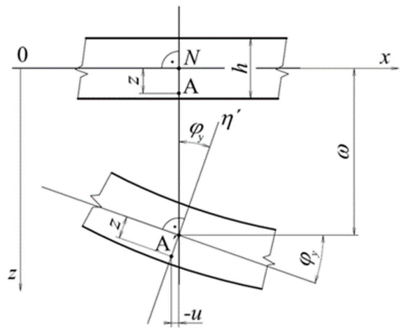
The above relations are based on the analysis of the displacement of the general point A of the normal to the median surface at the distance z (Figure 3).

After deformation of the plate due to the excitation load, the tangent to the median surface at point A rotates by an angle φ with respect to both the x-axis and the y-axis. Then, the displacements in the direction of the x and y axes can be described by relations using the angles of rotation φ_x and φ_y

$$u=-z·{\phi }_x,\hspace{1em}v=-z·{\phi }_y.$$

(11)

$${\phi }_x=\frac{\partial w}{\partial x}, \hspace{1em}{\phi }_y=\frac{\partial w}{\partial y}.$$

(12)

where the z-axis displacement is a function w = w(x,y).

Then, using Equations (10)–(12), Equation (6) can be rearranged to the form

$$\begin{array}{c}{\sigma }_x=\frac{-z{.E}_x}{{1 - \mu }_{xy}{\mu }_{yx}}\left(\frac{{\partial }^{2}w}{\partial x^2}{+\mu }_{yx}\frac{{\partial }^{2}w}{\partial y_2}\right){, \sigma }_{ y }=\frac{-z{.E}_y}{{1 - \mu }_{xy}{\mu }_{yx}}\left(\frac{{\partial }^{2}w}{\partial y^2}{+\mu }_{xy}\frac{{\partial }^{2}w}{\partial x^2}\right),\\ {\tau }_{xy}=-2z·G_{xy}\frac{{\partial }^{2}w}{\partial x\partial y}.\end{array}$$

(13)

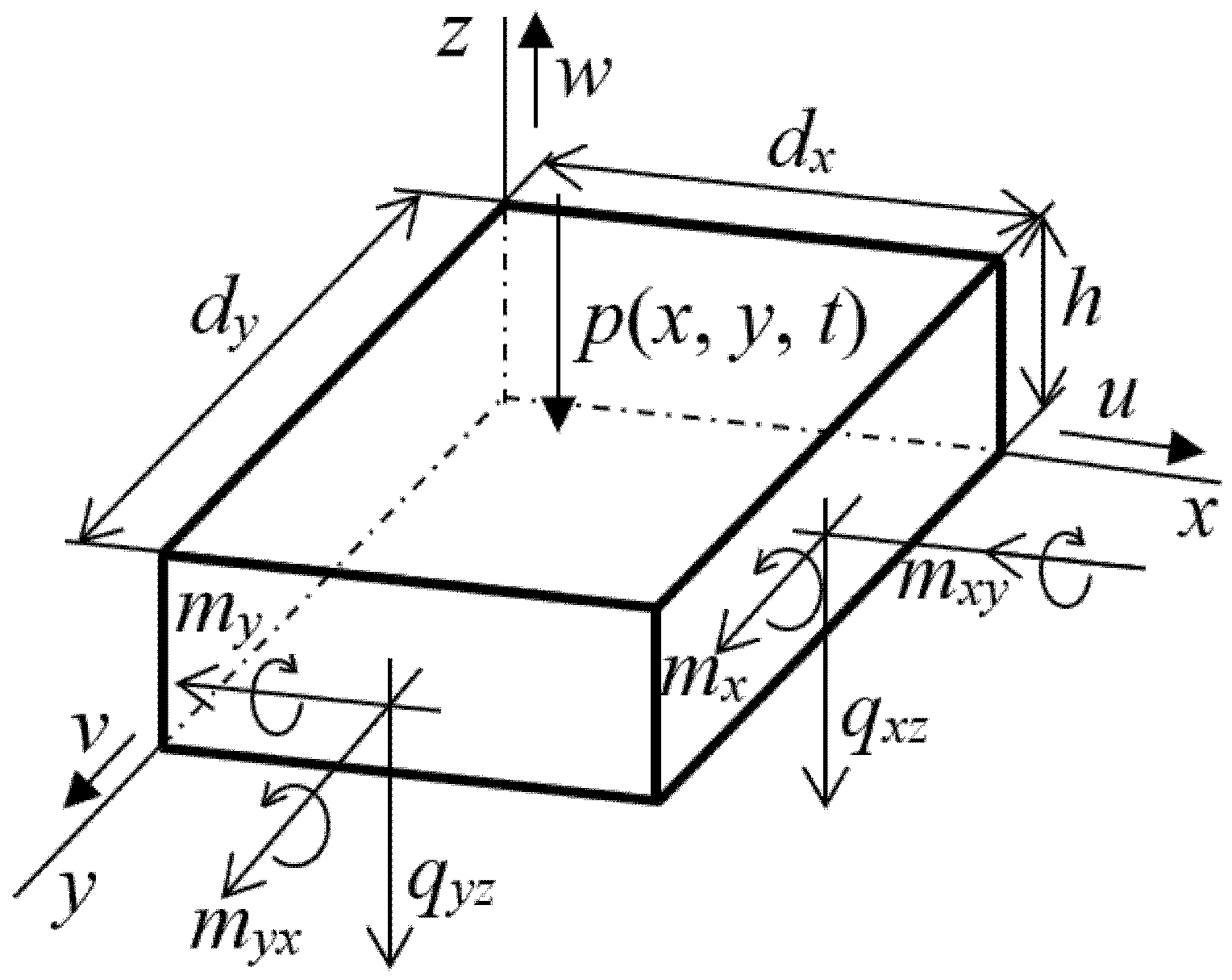
The three degrees of freedom of the plate element, i.e., the displacement w in the z-axis direction, the rotation around the x-axis by the angle φ_x and the rotation around the y-axis by the angle φ_y, correspond to the three motion equations of forces in the z-direction and moments to axes parallel to the x and y directions.

In thin plate theory, these equations of motion are usually formulated in integral form for the plate element dx × dy × h, using specific shear forces and bending and torsional moments (Figure 4).

The specific shear forces in the z direction act in a plane perpendicular to the axis x and y.

$$q_{xz}={{\displaystyle \int }}_{-\frac{h}{2}}^{+\frac{h}{2}}{\tau }_{xz}·{dz,\hspace{1em}q}_{yz}={{\displaystyle \int }}_{-\frac{h}{2}}^{+\frac{h}{2}}{\tau }_{yz}·dz.$$

(14)

Specific bending moment (m_x) acting in a plane parallel to the yz plane whose vector is parallel to the y-axis, specific bending moment (m_y) acting in a plane parallel to the xz plane, the vector parallel to the x-axis and specific torques (m_xy = m_yx) acting in planes of the element parallel to the planes xz and yz, whose vectors are perpendicular to these planes are defined:

$$m_x={{\displaystyle \int }}_{-\frac{h}{2}}^{+\frac{h}{2}}{\sigma }_x·z·{dz,\hspace{1em}m}_y={{\displaystyle \int }}_{-\frac{h}{2}}^{+\frac{h}{2}}{\sigma }_y·z·{dz,\hspace{1em}m}_{xy}{=m}_{yx}={{\displaystyle \int }}_{-\frac{h}{2}}^{+\frac{h}{2}}{\tau }_{xy}·z·dz.$$

(15)

These specific moments can be expressed with (13) as a function of the displacements

$$\begin{array}{c}{m}_x{=-D}_x\left(\frac{{\partial }^{2}w}{\partial x^2}{+\mu }_{yx}\frac{{\partial }^{2}w}{\partial y^2}\right){,\hspace{1em}\mathrm{where}\hspace{1em}D}_x=\frac{E_x{h}^3}{12\left({1-\mu }_{xy}{\mu }_{yx}\right)},\\ m_y=-D_y\left(\frac{{\partial }^{2}w}{\partial y^2}+{\mu }_{xy}\frac{{\partial }^{2}w}{\partial x^2}\right),\hspace{1em}\mathrm{where}\hspace{1em}{ D}_y=\frac{E_y{h}^3}{12\left({1-\mu }_{xy}{\mu }_{yx}\right)},\\ m_{xy}{=-2D}_{xy}\frac{{\partial }^{2}w}{\partial x\partial y},\hspace{1em}\mathrm{where}\hspace{1em} D_{xy}=\frac{G_{xy}{h}^3}{12}.\end{array}$$

(16)

where D_x, D_y—stiffness modules in the direction x and y, D_xy—torsional stiffness modulus.

After further modifications, three equations of motion can be formulated for the forces and moments acting on the plate element dxdyh.

$$\begin{array}{c}\frac{\partial q_{xz}}{\partial x}+\frac{\partial q_{yz}}{\partial y}+p(x,y,t)=\rho h\frac{{\partial }^{2}w}{\partial t^2},\hfill \\ q_{xy}=-\frac{\partial m_x}{\partial x}-\frac{\partial m_{xy}}{\partial y}{=J}_p\frac{{\partial }^2{\varphi }_x}{\partial t^2}{,\hspace{1em}\mathrm{where}\hspace{1em}J}_{\rho }=\rho \frac{h^3}{12}=\frac{d^2{J}_x}{dxdy}=\frac{d^2{J}_y}{dxdy}, \hfill \\ q_{yz}=-\frac{\partial m_y}{\partial y}-\frac{\partial m_{yx}}{\partial x}{=J}_p\frac{{\partial }^2{\varphi }_y}{\partial t^2}. \hfill \end{array}$$

(17)

where J_p—inertia material moment of the element dxdyh in axis x, or y, passing through the center of the element provided dx < h, dy < h, h—plate thickness, p—the function of the excitation load, ρ—plate density.

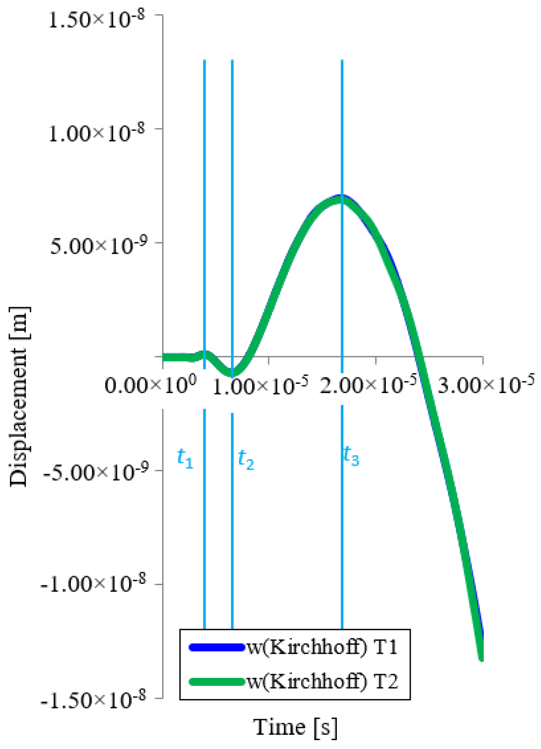
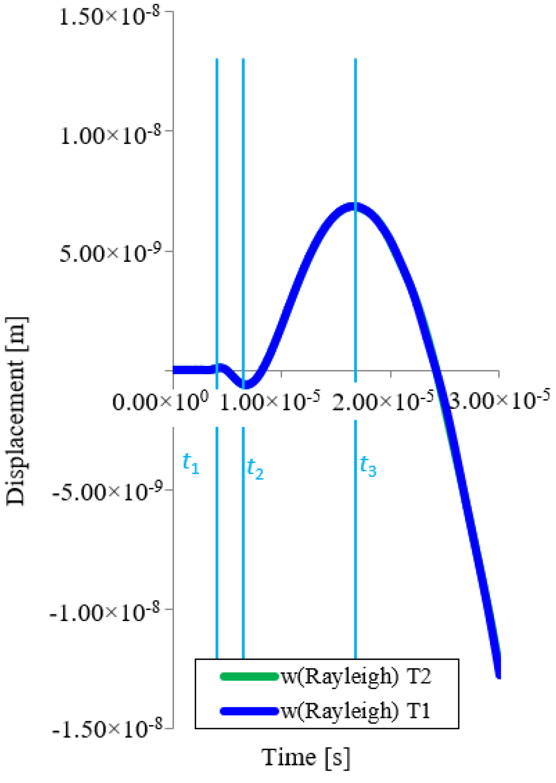
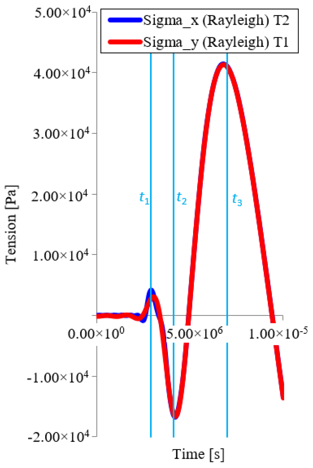
For moment equations, the right side respects the effect of the rotation of the plate element around the x and y axis—Rayleigh’s model. For J_p = 0. These equations have the character of moment-static equilibrium, when the effect of inertial moments, or cross-section rotation are neglected, which corresponds to the original Kirchhoff model.

By further arrangement (17) and using (12), (16) we get for Rayleigh’s model (J_p ≠ 0)

$$\begin{array}{c}{q}_{xz}=\frac{\partial }{\partial x}\left[J_{\rho }\frac{{\partial }^{2}w }{\partial t^2}{- D}_x\frac{{\partial }^{2}w}{\partial x^2}-D\frac{{\partial }^{2}w}{\partial y^2}\right]{, \mathrm{where} D=D}_x{\mu }_{yx}{+2D}_{xy}{=D}_y{\mu }_{xy}{+2D}_{xy},\hfill \\ q_{yz}=\frac{\partial }{\partial y}\left[J_{\rho }\frac{{\partial }^{2}w}{\partial t^2}{ - D}_y\frac{{\partial }^{2}w}{\partial y^2}-D\frac{{\partial }^{2}w}{\partial x^2}\right]. \hfill \end{array}$$

(18)

For the Kirchhoff model J_p = 0 and relations for q_xz and q_yz are clear. Substituting (18) into (17) we get for the displacement w = w(x,y,t)

$$D_x\frac{{\partial }^{4}w}{\partial x^4}+2D\frac{{\partial }^{4}w}{\partial x^2\partial y^2}{+D}_y\frac{{\partial }^{4}w}{\partial y^4}+\frac{{\partial }^2}{\partial t^2} \left[{\rho hw - J}_{\rho }\Delta w\right]=p\left(x,y,t\right).$$

(19)

By solution (19), e.g., by Fourier method we get for w

w(x,y,t) = X(x)Y(y)T(t)

(20)

Substituting (20) into (19) and arrangement we get

$$\begin{array}{c}\frac{{\partial }^{2}T\left(t\right)}{\partial t^2}\left[{\rho h-J}_{\rho }\left(\frac{{\partial }^{2}X\left(x\right)}{\partial x^2}\frac{1}{X\left(x\right)}+\frac{{\partial }^{2}Y\left(y\right)}{\partial y^2}\frac{1}{Y\left(y\right)}\right)\right]+\\ +\left[D_x\frac{{\partial }^{4}X\left(x\right)}{\partial x^4}\frac{1}{X\left(x\right)}+2D\frac{{\partial }^{2}X\left(x\right)}{\partial x^2}\frac{{\partial }^{2}Y\left(y\right)}{\partial y^2}\frac{1}{X\left(x\right)Y\left(y\right)}{+D}_y\frac{{\partial }^{4}Y\left(y\right)}{\partial y^4}\frac{1}{Y\left(y\right)}\right]T\left(t\right)=\\ \frac{p\left(x,y,t\right)}{X\left(x\right)Y\left(y\right)}\end{array}$$

(21)

We determine the functions X(x) and Y(y) from the relations

$$\begin{array}{c}\frac{{\partial }^{2n}X\left(x\right)}{\partial x^{2n}}={\left(-1\right)}^n{\alpha }^{2n}X\left(x\right),\hspace{1em}\frac{{\partial }^{2n}Y\left(y\right)}{\partial y^{2n}}={\left(-1\right)}^n{ \beta }^{2n}Y\left(y\right),\\ \mathrm{resp}.\\ \frac{{\partial }^{2n}X\left(x\right)}{\partial x^{2n}}{=\alpha }^{2n}X\left(x\right),\hspace{1em}\frac{{\partial }^{2n}Y\left(y\right)}{\partial y^{2n}}{=\beta }^{2n} Y\left(y\right),\end{array}$$

(22)

where α and β are constants, X(x), Y(y) are functions of coordinates that describe the geometry of the plate deformation and must also satisfy the boundary conditions [19,20].

By further arrangement and application of the boundary conditions, a relation is derived for the individual functions X(x) and Y(y) in the form

$${X\left(x\right)=\sin \alpha }_{n}x=\sin \frac{n\pi }{a}{x,\hspace{1em}Y\left(y\right)=\sin \beta }_{m}y=\sin \frac{m\pi }{b}y.$$

(23)

After substituting and arrangement, the function w(x,y,t)

$${w=w (x,y,t)=T\left(t\right) \sin \alpha }_n{ \sin \beta }_{m}y=T\left(t\right) \sin \frac{n\pi x}{a} \sin \frac{m\pi y}{b}.$$

(24)

Substituting (24) into (20) and adjusting, we get an ordinary differential equation for the function T(t):

$$\frac{d^{2}T\left(t\right)}{{dt}^2}{+\omega }^{2}T\left(t\right)=0,$$

(25)

where

$${\omega }^{2 }=\frac{D_x{\alpha }^4{+2D\alpha }^2{\beta }^2{+D}_y{\beta }^4}{{\rho h+J}_{\rho }\left({\alpha }^2{+\beta }^2\right)}.$$

(26)

which is the equation of free harmonic oscillating motion.

Then, the external load p (x,y,t) can be expressed in the form

$${p (x,y,t)=F}_0{ X}_{F }{\left(x\right) Y}_F{ \left(y\right) T}_{F }\left(t\right),$$

(27)

where X_F(x) and Y_F(y) are geometric load distribution characteristics, T_F(t)—dimensionless function of time, and F₀—maximum value of external excitation load.

For further solutions using the previous relationships, the dimensionless load parameter in the shape is determined:

$$p_{\mathrm{mn}}=\underset{0}{\overset{a}{{\displaystyle \int }}}\underset{0}{\overset{b}{{\displaystyle \int }}}{X}_F \left(x\right){ Y}_F \left(y\right){ \sin \alpha }_n{ x \sin \beta }_m y dx dy.$$

(28)

The external excitation load always acts on the upper (face) surface of the plate in a certain small area of different shape (Figure 5). The continuous load has different intensities. The problem is if we want to compare the theoretical results of the analysis of stress wave propagation (point load) with the experimental solution (continuous load in the surface), because the point load cannot be realized in the experiment.

When solving oscillation of plates, we are interested in the time course of the deformation of a thin plate caused by the excitation load, i.e., the function w = w(x,y,t). This solution, using the previous relationships and the unit jump function, can be obtained in the form of a double series:

$$w=w\left(x,y,t\right)={\displaystyle \sum }_{m=1}^{\infty }{\displaystyle \sum }_{n=1}^{\infty }{T}_{mn}({t)X}_{mn}({x)Y}_{mn}\left(y\right)$$

(29)

2.2. Analytical Solution of Geometric Models of Thin Isotropic Plates

As part of the solution of stress wave propagation in thin isotropic plates, we dealt with the solution of the basic geometric model of Kirchhoff and Rayleigh. Both geometric models were solved for Hook’s material model. The analytical solution is based on the basic assumptions of a plate with dimensions a × b × h supported and fixed around the perimeter. The plate was loaded with a vertical force in the geometric center of the plate by a continuous load acting on a surface of radius c. The basic relations on which the analytical solution of both models is based were derived in the previous section.

2.2.1. Kirchhoff’s Model

Kirchhoff’s model is the simplest model of a thin plate. In this model, only displacements and their corresponding tangent rotations and inertial effects are considered.

• Displacements w, u, v in axis z, x, y, respectively, are defined:

  $$\begin{array}{c}w=w\left(x,y,t\right)=\frac{16}{abc}\frac{F_0}{\rho h}{\displaystyle {\displaystyle \sum }_{m=1}^{\infty }}{\displaystyle {\displaystyle \sum }_{n=1}^{\infty }}\frac{J_1\left({\gamma }_{mn}c\right)}{{\gamma }_{mn}}\frac{\sin {\alpha }_n{x}_{F }\cos {\beta }_m{y}_F}{{\omega }_{mn}^2}\sin {\alpha }_{n}x \sin {\beta }_{m}y {\sin }^2\frac{{\omega }_{mn}}{2}t\\ {\omega }_{mn}=\left({\alpha }_n^2{+\beta }_m^2\right)\sqrt{\frac{D}{\rho h}}=\left({\alpha }_n^2{+\beta }_m^2\right)\frac{c h}{\sqrt{12}}\hspace{1em}D=\frac{{E h}^3}{{12 (1 - \mu }^2)}\\ {\gamma }_{mn}=\sqrt{{\alpha }_n^2{+\beta }_m^2}{\hspace{1em}\alpha }_n=n\frac{\pi }{a}{\hspace{1em}\beta }_m=m\frac{\pi }{b}\end{array}$$

  (30)

  $${ u=-z\phi }_x=-\frac{16z}{abc}\frac{F_0}{\rho h}{\displaystyle \sum }_{m=1}^{\infty }{\displaystyle \sum }_{n=1}^{\infty }\frac{J_1\left({\gamma }_{mn}c\right)}{{\gamma }_{mn}}\frac{{\alpha }_n}{{\omega }_{mn}^2}{\sin \alpha }_n{x}_{F }{\sin \beta }_m{y}_{F }{\cos \alpha }_n{x \sin \beta }_m{y \sin }^2\frac{{\omega }_{mn}}{2}t·$$

  (31)

  $${v=-z\phi }_y=-\frac{16z}{abc}\frac{F_0}{\rho h}{\displaystyle \sum }_{m=1}^{\infty }{\displaystyle \sum }_{n=1}^{\infty }\frac{J_1\left({\gamma }_{mn}c\right)}{{\gamma }_{mn}}\frac{{\beta }_m}{{\omega }_{mn}^2}{\sin \alpha }_n{x}_{F }{\sin \beta }_m{y}_F{ \sin \alpha }_n{x \cos \beta }_m{y \sin }^2\frac{{\omega }_{mn}}{2}t$$

  (32)

  where angles of tangents rotation φ_x and φ_y

  $$\begin{array}{c}{\phi }_x=\frac{\partial w}{\partial x}=\frac{16}{abc}\frac{F_0}{\rho h}{\displaystyle {\displaystyle \sum }_{m=1}^{\infty }}{\displaystyle {\displaystyle \sum }_{n=1}^{\infty }}\frac{J_1\left({\gamma }_{mn}c\right)}{{\gamma }_{mn}}\frac{{\alpha }_n}{{\omega }_{mn}^2}{ \sin \alpha }_n{x}_{F }{\sin \beta }_m{y}_F{ \cos \alpha }_n{x \sin \beta }_m{y \sin }^2\frac{{\omega }_{mn}}{2}t\end{array}$$

  (33)

  $$\begin{array}{c}{\phi }_y=\frac{\partial w}{\partial y}=\frac{16}{abc}\frac{F_0}{\rho h}{\displaystyle {\displaystyle \sum }_{m=1}^{\infty }}{\displaystyle {\displaystyle \sum }_{n=1}^{\infty }}\frac{J_1\left({\gamma }_{mn}c\right)}{{\gamma }_{mn}}\frac{{\beta }_m}{{\omega }_{mn}^2}{ \sin \alpha }_n{x}_{F }{\sin \beta }_m{y}_F{ \sin \alpha }_n{x \cos \beta }_m{y \sin }^2\frac{{\omega }_{mn}}{2}t\end{array}$$

  (34)

• The velocities $\stackrel{·}{u}$, $\stackrel{·}{v}$, $\stackrel{·}{w}$ in the direction of the individual axes are obtained by deriving the displacements in these axes according to time:

$$\dot{u} =\frac{\partial u}{\partial t}=-\frac{8z}{abc}\frac{F_0}{\rho h}{\displaystyle \sum }_{m=1}^{\infty }{\displaystyle \sum }_{n=1}^{\infty }\frac{J_1\left({\gamma }_{mn}c\right)}{{\gamma }_{mn}}\frac{{\alpha }_n}{{\omega }_{mn}}{ \sin \alpha }_n{x}_{F }{\sin \beta }_m{y}_F{ \cos \alpha }_n{x \sin \beta }_m{y \sin \omega }_{mn}t$$

(35)

$$\dot{v} =\frac{\partial v}{\partial t}=-\frac{8z}{abc}\frac{F_0}{\rho h}{\displaystyle \sum }_{m=1}^{\infty }{\displaystyle \sum }_{n=1}^{\infty }\frac{J_1\left({\gamma }_{mn}c\right)}{{\gamma }_{mn}}\frac{{\beta }_m}{{\omega }_{mn}}{ \sin \alpha }_n{x}_{F }{\sin \beta }_m{y}_F{ \sin \alpha }_n{x \cos \beta }_m{y \sin \omega }_{mn}t$$

(36)

$$\dot{w}=\frac{\partial w}{\partial t}=-\frac{8z}{abc}\frac{F_0}{\rho h}{\displaystyle \sum }_{m=1}^{\infty }{\displaystyle \sum }_{n=1}^{\infty }\frac{J_1\left({\gamma }_{mn}c\right)}{{\gamma }_{mn}}\frac{{\sin \alpha }_n{x}_F{ \sin \beta }_m{y}_F}{{\omega }_{mn}}{\sin \alpha }_n{x \sin \beta }_m{y \sin \omega }_{mn}t$$

(37)

• Due to the deflection, which is caused by the impact of the load body on the plate, bending stresses also arise in the plate σ_x, σ_y, defined in form

$$\begin{array}{c}{\sigma }_x\left(x,y,z,t\right)=\frac{Ez}{1-{\mu }^2}\frac{16}{abc}\frac{F_0}{\rho h}{\displaystyle {\displaystyle \sum }_{m=1}^{\infty }}{\displaystyle {\displaystyle \sum }_{n=1}^{\infty }}\frac{J_1\left({\gamma }_{mn}c\right)}{{\gamma }_{mn}}\frac{{\alpha }_n^2+\mu {\beta }_m^2}{{\omega }_{mn}^2}\sin {\alpha }_n{x}_{F }\sin {\beta }_m{y}_F \sin {\alpha }_{n}x \\ ·{ \sin \beta }_m{y \sin }^2\frac{{\omega }_{mn}}{2}t\end{array}$$

(38)

$$\begin{array}{c}{\sigma }_y\left(x,y,z,t\right)=\frac{Ez}{1-{\mu }^2}\frac{16}{abc}\frac{F_0}{\rho h}{\displaystyle {\displaystyle \sum }_{m=1}^{\infty }}{\displaystyle {\displaystyle \sum }_{n=1}^{\infty }}\frac{J_1\left({\gamma }_{mn}c\right)}{{\gamma }_{mn}}\frac{{\beta }_m^2+\mu {\alpha }_n^2}{{\omega }_{mn}^2}\sin {\alpha }_n{x}_F \sin {\beta }_m{y}_F \sin {\alpha }_{n}x \\ ·{ \sin \beta }_m{y \sin }^2\frac{{\omega }_{mn}}{2}t\end{array}$$

(39)

• Shear stress τ_xy = τ_yx by torque

  $$\begin{array}{c}{\tau }_{xy}\left(x,y,z,t\right)=-zG\frac{32}{abc}\frac{F_0}{\rho h}{\displaystyle {\displaystyle \sum }_{m=1}^{\infty }}{\displaystyle {\displaystyle \sum }_{n=1}^{\infty }}\frac{J_1\left({\gamma }_{mn}c\right)}{{\gamma }_{mn}}\frac{\alpha \beta }{{\omega }_{mn}^2}\sin {\alpha }_n{x}_{F }\sin {\beta }_m{y}_F \cos {\alpha }_{n}x\\ ·\cos {\beta }_{m}y {\sin }^2\frac{{\omega }_{mn}}{2}t\end{array}$$

  (40)

  and shear stresses τ_xz, τ_yz by normal forces

  $$\begin{array}{c}{\tau }_{xz}\left(x,y,z,t\right)=\left[1-{\left(\frac{2z}{h}\right)}^2\right]\frac{2F_{0}h{c}^2}{abc}{\displaystyle {\displaystyle \sum }_{m=1}^{\infty }}{\displaystyle {\displaystyle \sum }_{n=1 }^{\infty }}\frac{J_1\left({\gamma }_{mn}c\right)}{{\gamma }_{mn}}\frac{{\alpha }_n\left({\alpha }_n^2+{\beta }_m^2\right)}{{\omega }_{mn}^2}\sin {\alpha }_n{x}_F \sin {\beta }_m{y}_F\\ · {\cos \alpha }_n{x \sin \beta }_m{y \sin }^2\frac{{\omega }_{mn}}{2}t\end{array}$$

  (41)

  $$\begin{array}{c}{\tau }_{yz}\left(x,y,z,t\right)=\left[1-{\left(\frac{2z}{h}\right)}^2\right]\frac{2F_{0}h{c}^2}{abc}{\displaystyle {\displaystyle \sum }_{m=1}^{\infty }}{\displaystyle {\displaystyle \sum }_{n=1 }^{\infty }}\frac{J_1\left({\gamma }_{mn}c\right)}{{\gamma }_{mn}}\frac{{\beta }_m\left({\alpha }_n^2+{\beta }_m^2\right)}{{\omega }_{mn}^2}\sin {\alpha }_n{x}_F \sin {\beta }_m{y}_F\\ · {\sin \alpha }_n{x \cos \beta }_m{y \sin }^2\frac{{\omega }_{mn}}{2}t\end{array}$$

  (42)

  where a, b, h—plate dimensions, c—radius of circular load, ρ—plate density, F₀—loading force, J₁(γ_mnc)—Bessel function of the first kind, for argument γ_mnc, α, β—constants, m, n—matric elements, x_F, y_F—coordinates of circular load, ω_mn—eigen frequency, t—time, D—stiffness module, E,—Young’s modulus, G—shear modulus, and μ—shear viscosity coefficient.

2.2.2. Rayleigh’s Model

Kirchhoff’s original theory of thin plate loading was modified and extended by Rayleigh about influence the rotation of cross sections. This new theory considers the influence of the rotation of the cross-sections when determining the displacements in the direction of the axes, the rotation of the tangents and the inertial effects.

• Displacements w, u, v in axis z, x, y, respectively, are defined:

  $$\begin{array}{c}w=w\left(x,y,t\right)=\frac{16}{abc}\frac{F_0}{\rho h}{\displaystyle {\displaystyle \sum }_{m=1}^{\infty }}{\displaystyle {\displaystyle \sum }_{n=1}^{\infty }}\frac{J_1\left({\gamma }_{mn}c\right)}{{\gamma }_{mn}}\frac{\sin {\alpha }_n{x}_{F }\cos {\beta }_m{y}_F}{\left[\frac{h^2}{12}\left({\alpha }_n^2+{\beta }_m^2\right)+1\right]{\omega }_{mn}^2}\sin {\alpha }_{n}x \sin {\beta }_{m}y·\\ ·{\sin }^2\frac{{\omega }_{mn}}{2}t\\ {\omega }_{mn}=\frac{\left({\alpha }_n^2+{\beta }_m^2\right)}{\sqrt{\frac{h^2}{12}\left({\alpha }_n^2+{\beta }_m^2\right)+1}}\sqrt{\frac{D}{\rho h}}=\frac{\left({\alpha }_n^2+{\beta }_m^2\right)}{\sqrt{\frac{h^2}{12}\left({\alpha }_n^2+{\beta }_m^2\right)+1}}\frac{c h}{\sqrt{12}}\hspace{1em}D=\frac{{E h}^3}{{12 (1 - \mu }^2)}\\ {\gamma }_{mn}=\sqrt{{\alpha }_n^2{+\beta }_m^2}{\hspace{1em}\alpha }_n=n\frac{\pi }{a}{ \beta }_m=m\frac{\pi }{b}\end{array}$$

  (43)

  $${ u=-z\phi }_x=-\frac{16z}{abc}\frac{F_0}{\rho h}{\displaystyle \sum }_{m=1}^{\infty }{\displaystyle \sum }_{n=1}^{\infty }\frac{J_1\left({\gamma }_{mn}c\right){ \alpha }_n{\sin \alpha }_n{x}_{F }{\sin \beta }_m{y}_{F }}{{\gamma }_{mn}\left[\frac{h^2}{12}\left({\alpha }_n^2+{\beta }_m^2\right)+1\right]{\omega }_{mn}^2}{\cos \alpha }_n{x \sin \beta }_m{y \sin }^2\frac{{\omega }_{mn}}{2}t$$

  (44)

  $${ v=-z\phi }_y=-\frac{16z}{abc}\frac{F_0}{\rho h}{\displaystyle \sum }_{m=1}^{\infty }{\displaystyle \sum }_{n=1}^{\infty }\frac{J_1\left({\gamma }_{mn}c\right){\beta }_m{\sin \alpha }_n{x}_{F }{\sin \beta }_m{y}_{F }}{{\gamma }_{mn}\left[\frac{h^2}{12}\left({\alpha }_n^2+{\beta }_m^2\right)+1\right]{\omega }_{mn}^2}{\sin \alpha }_n{x \cos \beta }_m{y \sin }^2\frac{{\omega }_{mn}}{2}t$$

  (45)

  where angles of tangents rotation φ_x and φ_y

  $$\begin{array}{c}{\phi }_x=\frac{\partial w}{\partial x}=\frac{16}{abc}\frac{F_0}{\rho h}{\displaystyle {\displaystyle \sum }_{m=1}^{\infty }}{\displaystyle {\displaystyle \sum }_{n=1}^{\infty }}\frac{J_1\left({\gamma }_{mn}c\right){\alpha }_n{\sin \alpha }_n{x}_{F }{\sin \beta }_m{y}_F}{{\gamma }_{mn}\left[\frac{h^2}{12}\left({\alpha }_n^2+{\beta }_m^2\right)+1\right]{\omega }_{mn}^2}{\cos \alpha }_n{x \sin \beta }_m{y \sin }^2\frac{{\omega }_{mn}}{2}t\end{array}$$

  (46)

  $$\begin{array}{c}{\phi }_y=\frac{\partial w}{\partial y}=\frac{16}{abc}\frac{F_0}{\rho h}{\displaystyle {\displaystyle \sum }_{m=1}^{\infty }}{\displaystyle {\displaystyle \sum }_{n=1}^{\infty }}\frac{J_1\left({\gamma }_{mn}c\right){\beta }_m{\sin \alpha }_n{x}_{F }{\sin \beta }_m{y}_F}{{\gamma }_{mn}\left[\frac{h^2}{12}\left({\alpha }_n^2+{\beta }_m^2\right)+1\right]{\omega }_{mn}^2}{\sin \alpha }_n{x \cos \beta }_m{y \sin }^2\frac{{\omega }_{mn}}{2}t\end{array}$$

  (47)

• The velocities $\stackrel{·}{u}$, $\stackrel{·}{v}$, $\stackrel{·}{w}$ in the direction of the individual axes are obtained by deriving the displacements in these axes according to time:

$$\dot{u} =\frac{\partial u}{\partial t}=-\frac{8z}{abc}\frac{F_0}{\rho h}{\displaystyle \sum }_{m=1}^{\infty }{\displaystyle \sum }_{n=1}^{\infty }\frac{J_1\left({\gamma }_{mn}c\right){\alpha }_n{\sin \alpha }_n{x}_{F }{\sin \beta }_m{y}_F}{{\gamma }_{mn}\left[\frac{h^2}{12}\left({\alpha }_n^2+{\beta }_m^2\right)+1\right]{\omega }_{mn}^2}{ \cos \alpha }_n{x \sin \beta }_m{y \sin \omega }_{mn}t$$

(48)

$$\dot{v} =\frac{\partial v}{\partial t}=-\frac{8z}{abc}\frac{F_0}{\rho h}{\displaystyle \sum }_{m=1}^{\infty }{\displaystyle \sum }_{n=1}^{\infty }\frac{J_1\left({\gamma }_{mn}c\right){\beta }_m{\sin \alpha }_n{x}_{F }{\sin \beta }_m{y}_F}{{\gamma }_{mn}\left[\frac{h^2}{12}\left({\alpha }_n^2+{\beta }_m^2\right)+1\right]{\omega }_{mn}^2}{ \sin \alpha }_n{x \cos \beta }_m{y \sin \omega }_{mn}t$$

(49)

$$\dot{w}=\frac{\partial w}{\partial t}=-\frac{8z}{abc}\frac{F_0}{\rho h}{\displaystyle \sum }_{m=1}^{\infty }{\displaystyle \sum }_{n=1}^{\infty }\frac{J_1\left({\gamma }_{mn}c\right){\sin \alpha }_n{x}_F{ \sin \beta }_m{y}_F}{{\gamma }_{mn}\left[\frac{h^2}{12}\left({\alpha }_n^2+{\beta }_m^2\right)+1\right]{\omega }_{mn}^2}{\sin \alpha }_n{x \sin \beta }_m{y \sin \omega }_{mn}t$$

(50)

• Bending stresses σ_x, σ_y are determined from relations

$$\begin{array}{c}{\sigma }_x\left(x,y,z,t \right)=\frac{Ez}{1-{\mu }^2}\frac{16}{abc}\frac{F_0}{\rho h}{\displaystyle {\displaystyle \sum }_{m=1}^{\infty }}{\displaystyle {\displaystyle \sum }_{n=1}^{\infty }}\frac{J_1\left({\gamma }_{mn}c\right){\alpha }_n^2+\mu {\beta }_m^2}{{\gamma }_{mn}\left[\frac{h^2}{12}\left({\alpha }_n^2+{\beta }_m^2\right)+1\right]{\omega }_{\mathrm{mn}}^2}\sin {\alpha }_n{x}_{F } ·\\ \sin {\beta }_m{y}_F \sin {\alpha }_{n}x{\sin \beta }_m{y \sin }^2\frac{{\omega }_{mn}}{2}t\end{array}$$

(51)

$$\begin{array}{c}{\sigma }_y\left(x,y,z,t\right)=\frac{Ez}{1-{\mu }^2}\frac{16}{abc}\frac{F_0}{\rho h}{\displaystyle {\displaystyle \sum }_{m=1}^{\infty }}{\displaystyle {\displaystyle \sum }_{n=1}^{\infty }}\frac{J_1\left({\gamma }_{mn}c\right){\beta }_m^2+\mu {\alpha }_n^2}{{\gamma }_{mn}\left[\frac{h^2}{12}\left({\alpha }_n^2+{\beta }_m^2\right)+1\right]{\omega }_{mn}^2}\sin {\alpha }_n{x}_F\cdot \\ · \sin {\beta }_m{y}_F \sin {\alpha }_{n}x {\sin \beta }_m{y \sin }^2\frac{{\omega }_{mn}}{2}t\end{array}$$

(52)

• Shear stress τ_xy = τ_yx by torque moment

  $$\begin{array}{c}{\tau }_{xy}\left(x,y,z,t\right)=-z{G}_{xy}\frac{32}{abc}\frac{F_0}{\rho h}{\displaystyle {\displaystyle \sum }_{m=1}^{\infty }}{\displaystyle {\displaystyle \sum }_{n=1}^{\infty }}\frac{J_1\left({\gamma }_{mn}c\right){\alpha }_n{\beta }_m}{{\gamma }_{mn}\left[\frac{h^2}{12}\left({\alpha }_n^2+{\beta }_m^2\right)+1\right]{\omega }_{mn}^2}\sin {\alpha }_n{x}_{F }\\ · \sin {\beta }_m{y}_F \cos {\alpha }_{n}x \cos {\beta }_{m}y {\sin }^2\frac{{\omega }_{mn}}{2}t\end{array}$$

  (53)

  and shear stress τ_xz, τ_yz by normal forces

  $$\begin{array}{c}{\tau }_{xz}\left(x,y,z,t\right)=\left[1-{\left(\frac{2z}{h}\right)}^2\right]\frac{24F_0}{abc}{\displaystyle {\displaystyle \sum }_{m=1}^{\infty }}{\displaystyle {\displaystyle \sum }_{n=1 }^{\infty }}\frac{J_1\left({\gamma }_{mn}c\right)}{{\gamma }_{mn}}\frac{{\alpha }_n}{h\left({\alpha }_n^2+{\beta }_m^2\right)\left[\frac{h^2}{12}\left({\alpha }_n^2+{\beta }_m^2\right)+1\right]}\\ · \sin {\alpha }_n{x}_F \sin {\beta }_m{y}_F{\cos \alpha }_n{x \sin \beta }_m{y \sin }^2\frac{{\omega }_{mn}}{2}t\end{array}$$

  (54)

  $$\begin{array}{c}{\tau }_{yz}\left(x,y,z,t\right)=\left[1-{\left(\frac{2z}{h}\right)}^2\right]\frac{24F_0}{abc}{\displaystyle {\displaystyle \sum }_{m=1}^{\infty }}{\displaystyle {\displaystyle \sum }_{n=1}^{\infty }}\frac{J_1\left({\gamma }_{mn}c\right)}{{\gamma }_{mn}}\frac{{\beta }_m}{h\left({\alpha }_n^2+{\beta }_m^2\right)\left[\frac{h^2}{12}\left({\alpha }_n^2+{\beta }_m^2\right)+1\right]}\\ ·\sin {\alpha }_n{x}_{F }\sin {\beta }_m{y}_F{\sin \alpha }_n{x \cos \beta }_m{y \sin }^2\frac{{\omega }_{mn}}{2}t\end{array}$$

  (55)

The notation in the above samples is the same as in the Kirchhoff model.

3. Solution and Discussion

A thin isotropic aluminum plate with dimensions a × b × h (a = 200 mm, b = 100 mm, and h = 2 mm) was solved, see Figure 6. The plate was made of unidirectionally rolled aluminum Al 99.9 (see material properties in

Table 1. Material parameters of aluminum plate.

Name	Notation	Unit	Value
Young’s module	E	Pa	7.1 × 1010
Poisson’s ratio	μ	-	0.34
Density	ρ	kg·m−3	2699

). We consider the plate embedded around the entire perimeter.

The mathematical solution was performed for the geometric model of Kirchhoff’s and Rayleigh’s and Hooke’s material model. The excitation is considered by an impact force of magnitude F = 1 N (Heaviside jump) in the geometric center C_R of the plate. The magnitude of the force does not affect the course of displacements, rotations, velocities, or stresses, only the magnitude of their maximum values. The propagation of the transverse wave in the direction of the x, y and z axes is solved at points T₁ and T₂ (the points are 20 mm far from the center of the impact and lie on the axes of symmetry of the plate). The wave propagates from the center to the embedded edges of the plate, where it reflects and returns. The solution is done only for times before the wave reach the edge of the plate.

The course of the propagating shock wave was determined according to the relations given in Section 2.2.1 and Section 2.2.2. The calculation was performed in the MATLAB software environment.

3.1. Kirchhoff’s Model—Results of the Solution

The results of the transverse wave displacements in the direction of the x, y, z axes—see Figure 7 and Figure 8.

Figure 7 and

Table 2. Displacement of wave in x (u) and y (v) axis direction in points T₁, T₂ (Kirchhoff).

Mark	Time	Displacement		Comparison
		u (T2)	v (T1)	Col. 4 − Col. 3	$\frac{\mathbf{Col}. 5}{\mathbf{Col}. 3}\mathit{·}100$
1	2	3	4	5	6
	[s]	[m]	[m]	[m]	[%]
t1	3.000 × 10−6	2.383 × 10−11	2.362 × 10−11	−0.021 × 10−11	0.9
t2	3.900 × 10−6	−1.336 × 10−11	−1.294 × 10−11	0.042 × 10−11	3.1
t3	5.400 × 10−6	4.647 × 10−11	4.716 × 10−11	0.069 × 10−11	1.5

show that the difference in wave propagation in the x and y axis directions is insignificant (T₁ and T₂). The course in both directions shows a very good agreement, as shown in Figure 7. The board material has identical properties in both directions (it is isotropic). Local extremes were reached at times t₁, t₂, t₃—see Table 2, where the difference in individual times is max. 3.1%.

The propagation of the wave in the z-axis shows a high agreement when viewed from the direction of the x and y axes, see

Table 3. Trend of wave in z (w) axis direction in point T₁, T₂ (Kirchhoff).

Mark	Time	Displacement		Comparison
		w (T2)	w (T1)	Col. 4 − Col. 3	$\frac{\mathbf{Col}. 5}{\mathbf{Col}. 3}\mathit{·}100$
1	2	3	4	5	6
	[s]	[m]	[m]	[m]	[%]
t1	4.000 × 10−6	1.284 × 10−10	1.284 × 10−10	0.000 × 10−10	0.0
t2	6.500 × 10−6	−6.864 × 10−10	−6.859 × 10−10	0.005 × 10−10	0.1
t3	1.680 × 10−5	6.966 × 10−10	6.939 × 10−10	−0.027 × 10−10	0.4

. The extremes that were achieved at point T₁ and T₂ are max. 0.4%.

Similar results were obtained for the wave propagation velocity, see Figure 9. After reaching the reverse side of the plate, the wave reflected from the edge, manifested in the oscillation of the velocity trend after time t₃.

The normal stress trend is also smooth until the reflected wave is captured. It is obvious that the normal stress shows a very good agreement in both directions, see Figure 10. Small inaccuracies before time t₁ are probably caused by inaccuracies in the Bessel function calculation.

3.2. Rayleigh’s Model—Results of the Solution

As mentioned above, Rayleigh extended Kirchhoff’s geometric model of the plate by the effect of the rotation of the cross sections of the plate. In the analytical solution of this model, the simplest material model was again used, i.e., Hooke’s model. Figure 11 shows the displacement in transverse wave in the x and y axis directions for point T₁ and T₂.

Figure 12 shows the course of the transverse displacement in the z-axis direction at points T₁ and T₂.

In

Table 4. Displacement by wave propagation in z (w) axis direction for points T₁ and T₂ (Rayleigh).

Mark	Time	Displacement		Comparison
		w (T2)	w (T1)	Col. 4 − Col. 3	$\frac{\mathbf{Col}. 5}{\mathbf{Col}. 3}\mathit{·}100$
1	2	3	4	5	6
	[s]	[m]	[m]	[m]	[%]
t1	4.000 × 10−6	5.259 × 10−11	5.437 × 10−10	0.178 × 10−10	3.40
t2	6.500 × 10−6	−6.132 × 10−10	−6.133 × 10−10	−0.001 × 10−10	0.1
t3	1.680 × 10−5	6.825 × 10−9	6.830 × 10−9	0.005 × 10−9	0.1

, the displacement by wave propagation in the z-axis direction at point T₁ and T₂ for times t₁, t₂ and t₃ is evaluated numerically. Figure 12 shows both waveforms simultaneously. It follows from Table 4 that the difference between the two points is the largest at time t₁, namely 3.4%. In the other two times, it is only 0.1%, which is a very good agreement. The differences can be attributed to the inaccuracies of the Bessel function calculation.

In the Figure 13, z-axis velocity profile at the T₁ and T₂ points is presented. From Figure 13, it can be seen that after passing the transverse wave through the thickness of the plate, it is reflected from the back and thus the time trend is deformed. Figure 13 again shows a very good agreement of the velocity across the plate at point T₁ and T₂.

Figure 14 shows the trend of normal stress in the x and y axis, i.e., σ_y at point T₁ (σ_x = 0) and σ_x at point T₂ (σ_y = 0). Figure 14 then compares stresses.

The above comparison shows that the transverse wave propagates from the point of impact along circular paths. At the point of plate support, the propagation of the transverse wave is reflected, and thus the courses of displacement and velocity are deformed. When the wave propagates across the plate, the reflection occurs in a disproportionately shorter time, because the excitation propagates in all directions at the same velocity and the reflection time depends only on the distance of the jamming point and the thickness of the plate. A similar conclusion can be formulated even in the case of wave propagation according to Kirchhoff, see Section 3.1.

3.3. Comparison of Kirchhoff’s and Rayleig’s Models

Rayleigh’s geometrical model, unlike Kirchhoff’s geometrical model, respects the influence of the cross-section rotation, as mentioned above. Since the same material model (Hooke’s) was used for both models in the analytical calculation, it is appropriate to perform a mutual comparison of displacements, velocities and stresses.

Figure 15a shows a comparison of the course of the transverse displacement in the direction of the y-axis at the point T₂ at time t₁, t₂, t₃. From the course of both displacements, it is evident that the differences are relatively significant and range from 55.1 to 107.7% (see

Table 5. Comparison v displacements in y-axis direction as a function of time for Kirchhoff’s and Rayleigh’s model at point T₁.

Mark	Time	Displacement		Comparison
		Kirchhoff	Rayleigh	Col. 4 − Col. 3	$\frac{\mathbf{Col}. 5}{\mathbf{Col}. 3}\mathit{·}100$
1	2	3	4	5	6
	10−6 [s]	10−10 [m]	10−10 [m]	10−10 [m]	[%]
t1	2.500	0.336	0.024	−0.312	92.9
t2	3.400	−1.294	0.099	1.393	107.7
t3	5.100	4.716	2.118	−2.598	55.1

). This is probably due to the use of a improved model (Rayleigh). Similarly, the deviations of the transverse wave in the x-axis (see Figure 15b) are significantly different for both models at different times and range from 6.3 to 90.4%, see

Table 6. Comparison u displacements in x-axis direction as a function of time for Kirchhoff’s and Rayleigh’s model at point T₂.

Mark	Time	Displacement		Comparison
		Kirchhoff	Rayleigh	Col. 4 − Col. 3	$\frac{\mathbf{Col}. 5}{\mathbf{Col}. 3}\mathit{·}100$
1	2	3	4	5	6
	10−6 [s]	10−10 [m]	10−10 [m]	10−10 [m]	[%]
t1	3.000	0.125	0.238	0.110	90.4
t2	3.900	−0.708	−1.246	−0.538	75.9
t3	5.400	4.373	4.647	0.274	6.30

.

With the displacement in the z-axis direction (Figure 16), it is evident that for both models, the agreement is very good for longer times (t₂, t₃), and difference is up to 10.6%. The bigger difference is only in the short time t₁, where it is about 58%. At both points, these differences are always almost identical (see

Table 7. Comparison of displacement w in the z axis as a function of time for Kirchhoff’s and Rayleigh’s model at point T₁.

Mark	Time	Displacement		Comparison
		Kirchhoff	Rayleigh	Col. 4 − Col. 3	$\frac{\mathbf{Col}. 5}{\mathbf{Col}. 3}\mathit{·}100$
1	2	3	4	5	6
	10−6 [s]	10−10 [m]	10−10 [m]	10−10 [m]	[%]
t1	4.000	0.128	0.054	−0.074	57.8
t2	6.500	−0.686	−0.613	0.073	10.6
t3	16.800	6.939	6.830	−0.109	1.60

and

Table 8. Comparison of displacement w in the z axis as a function of time for Kirchhoff’s and Rayleigh’s model at point T₂.

Mark	Time	Displacement		Comparison
		Kirchhoff	Rayleigh	Col. 4 − Col. 3	$\frac{\mathbf{Col}. 5}{\mathbf{Col}. 3}\mathit{·}100$
1	2	3	4	5	6
	10−6 [s]	10−10 [m]	10−10 [m]	10−10 [m]	[%]
t1	4.000	0.128	0.054	−0.075	58.6
t2	6.500	−0.686	−0.613	0.073	10.6
t3	16.800	6.966	6.825	−0.141	2.00

). The larger difference in time t₁ is probably due to the corrections used in the Rayleigh model. Thus, it can be said that Rayleigh’s model is more accurate—it shows a faster response to impact (the same in both directions).

From the comparison of the propagation of the transverse wave velocity in the x and y directions ($\stackrel{·}{u}$, $\stackrel{·}{v}$, see Figure 17), the velocities at time t₁ and t₂ differ quite considerably, when the Kirchhoff’s model acquires higher values. This is probably because considering the rotation of the cross sections, there is a greater loss of energy, and therefore less speed (Rayleigh).

Figure 18 shows a comparison of the z-axis propagation velocity in the z-axis direction at point T₁ and T₂. A comparison of Kirchhoff’s and Rayleigh’s models at time t₃ shows a very good agreement. This is mainly because the total displacement w in the direction of the z-axis is smaller compared to the displacement in the x-axis (25×) and the y-axis (50×), and therefore no such differences could have occurred.

Figure 19 shows comparison of the course of normal stresses in the x and y axes of both models. It is obvious that both courses show a relatively good agreement. The stress at time t₃ is slightly higher in the Rayleigh’s model, which is due to a more accurate calculation, which is given by the already mentioned correction.

4. Conclusions

The behavior of thin isotropic plates under impact loading was analytically derived in the paper. For a thin plate, we assumed three planes of symmetry and solved the relationships between stress components and deformations. Basic analytical methods, including matrix calculation, were used for the solution. The published solution is simplified, and some relationships arising from the context have been omitted. The basic geometric models of Kirchhoff and Rayleigh for Hooke’s material model were solved. This was followed by an analytical calculation for the plate according to Figure 6. The results obtained for the Kirchhoff model, i.e., the displacement of the transverse wave in the x and y direction (u and v) at points T₁ and T₂, are graphically shown in Figure 7. The displacements in the z axis are presented in Figure 8. The results for the velocity trends and normal stress in the given axes are also presented, even for the Rayleigh’s model. The next part is a graphical comparison of the calculated results of both models. A comparison of the results shows a relatively good agreement with the fact that the displacement of plate at specific place after time t₃ is already affected by the inclusion of the reflection of the waves from the point of support.

We assume that in the next stage, the analytical solution will continue with the model of Flügge and Timoshenko–Mindlin, with the last of these models being compared with the experiment. The reason is that the Timoshenko–Mindlin model is closest to reality, although even this model does not capture all aspects of the problem.

References

1. Chladni, E.F.F. Entdeckungen über die Theorie des Klanges; Weidmanns Erben und Reich: Leipzig, Germany, 1787; p. 90. [Google Scholar]
2. Bernoulli, J., II. Lettre sur l’élasticité. J. De Phys. De Rozier 1782, 21, 463–467. [Google Scholar]
3. Germain, M.-S. Récherches sur la Théorie des Surfaces Élastiques; Courcier, M.V., Ed.; Libraire Pour Les Sciences: Paris, France, 1821. [Google Scholar]
4. Kirchhoff, G. Ueber die Schwingungen einer kreisförmigen elastischen Scheibe. Ann. Der Phys. 1850, 157, 258–264. [Google Scholar] [CrossRef] [Green Version]
5. Volek, J.; Červ, F.; Valeš, J. Vlny v Tenké Ortotropní Desce (Model Kirchhoffův a Rayleigho) Generované Příčným Pulsním Zatížrním. In Proceedings of the Výpočtová Mechanika 2003, 19. Konference s Mezinárodní Účastí, Nečtiny, The Czech Republic, 3–15 November 2003. [Google Scholar]
6. Flügge, W. Die Ausbreitung von Biegung Wellen in Stäbau. Zeit. Angew; Bd.22; Mathematik Mechanik: Germany, 1942; pp. 312–318. [Google Scholar]
7. Timoshenko, S.; Woinowsky-Krieger, S. Theory of Plates and Shells, 1st ed.; McGraw-Hill Book Company: New York, NY, USA, 1940; p. 580. [Google Scholar]
8. Mindlin, R.D. Influence of Rotatory Inertia and Shear on Flexural Motions of Isotropic, Elastic plates. Appl. Mech. 1951, 18, 31–38. [Google Scholar] [CrossRef]
9. Hsu, M.-H. Vibration Analysis of Isotropic and Orthotropic Plates with Mixed Boundary Conditions. Tamkang J. Sci. Eng. 2003, 6, 217–226. [Google Scholar]
10. Vanam, B.; Inala, R. Static analysis of an isotropic rectangular plate using finite element method (FEM). J. Mech. Eng. Res. 2012, 4, 148–162. [Google Scholar]
11. Mohanty, S.C.; Ramu, I. Study of Free Vibration Analysis of Rectangular Plate Structures Using Finite Element Method. Procedia Eng. 2012, 38, 2758–2766. [Google Scholar]
12. Volek, J. Nestacionární Napjatost Tenké Desky Vyvolané Příčnou Osamělou Silou; Bulletin vědeckých, výzkumných a pedagogických prací ústavu za rok 2000, Ústav techniky a řízení výroby; UJEP: Ústí nad Labem, The Czech Republic, 2000. [Google Scholar]
13. Volek, J. Ráz a Přenos Impulsu v Soustavě Elastických a Viskoelastických Jedno a Dvourozměrných Těles; Závěrečná výzkumná práce pro ÚT ČSAV: Litoměřice, The Czech Republic, 1990. [Google Scholar]
14. Klimenda, F.; Soukup, J.; Zmindak, M. Deformation of Aluminium Plate. Manuf. Technol. 2016, 16, 124–129. [Google Scholar]
15. Klimenda, F.; Soukup, J. Modal Analysis of Thin Aluminium Plate. Procedia Eng. 2017, 177, 11–16. [Google Scholar] [CrossRef]
16. Chiker, Y.; Mourad, B.; Bouaziz, S.; Mouloud, G.; Amar, M.B.; Haddar, M. Free vibration analysis of hybrid laminated plates containing multilayer functionally graded carbon nanotube-reinforced composite plies using a layer-wise formulation. Arch. Appl. Mech. 2020, 91, 463–485. [Google Scholar] [CrossRef]
17. Mehar, K.; Mishra, P.K.; Panda, S.K. Numerical investigation of thermal frequency responses of graded hybrid smart nanocomposite (CNT-SMA-Epoxy) structure. Mech. Adv. Mater. Struc. 2021, 28, 2242–2254. [Google Scholar] [CrossRef]
18. Teotia, M.; Soni, R.K. Applications of Finite Element Modelling in Failure Analysis of Laminated Glass Composites: A Review. Eng. Fail. Anal. 2018, 94, 412–437. [Google Scholar] [CrossRef]
19. Mahabadi, R.K.; Shakeri, M.; Danesh, P.M. Free vibration of laminated composite plate with shape memory alloy fibers. Lat. Am. J. Solids Struct. 2016, 13, 314–330. [Google Scholar] [CrossRef] [Green Version]
20. Karimimahabadi, R.; Daneshpazhooh, M.; Shakeri, M. On the free vibration and design optimization of a shape memory alloy hybrid laminated composite plate. Acta Mech. 2021, 232, 1–21. [Google Scholar] [CrossRef]
21. Panc, V. Teorie Pružných Desek; Academia: Praha, The Czech Republic, 1970. [Google Scholar]
22. Sokolnikoff, I.S. Mathematical Theory of Elasticity; McGrow-Hill: New York, NY, USA, 1956. [Google Scholar]
23. Leitmann, M.J. The Linear Theory of Viscoelasticity; Encyklopedia of Physics: Berlin, Germany, 1973. [Google Scholar]
24. Klimenda, F. Ráz a Přenos Impulzu v Tenké Izotropní Desce. Ph.D. Thesis, FSI UJEP v Ústí nad Labem, Ústí nad Labem, The Czech Republic, 2018. [Google Scholar]
25. Wang, Z.; Ma, L. Effect of Thickness Stretching on Bending and Free Vibration Behaviors of Functionally Graded Graphene Reinforced Composite Plates. Appl. Sci. 2021, 11, 11362. [Google Scholar] [CrossRef]
Figure 1. Plate geometry and quantities definition (adapted from [5]). a, b, h—plate dimensions, c—impact body radius, F0—loading force of impact body, xF, yF—force coordinates, σx, σy—bending stress, τyx, τxy—torsional stress, τxz, τyz—shear stress.
Applsci 12 02493 g001
Figure 2. Hooke’s model of plate (adapted from [23]). E, G—Young’s and shear modulus, μ—normal viscosity coefficients.
Applsci 12 02493 g002
Figure 3. Element of plate—scheme. n, n’—normals, t, t´—tangents, u, w—displacement in x and y, φx, φy—rotation angles of cross-section in x and y, A, A´—investigated point, z—displacement of A, h—plate thickness.
Applsci 12 02493 g003
Figure 4. Shear forces and moments acting on the plate element.
Applsci 12 02493 g004
Figure 5. Plate excitation load variants. xFk, yFk—coordinates of the circular load, xF, yF—coordinates of single force loading, xFo, yFo—coordinates of the rectangular load, a, b, h—plate dimensions, p(x,y,t)—circular load, F(t)—single force loading, p(x,y) TF(t)—rectangular load, aFo, bFo—dimensions of rectangular load, c—radius of circular load.
Applsci 12 02493 g005
Figure 6. Solved model. CR—impact center, T1, T2—observed points, a—plate length, b—plate width, h—plate thickness.
Applsci 12 02493 g006
Figure 7. Displacement in the direction of the x and y axes for point T1 and T2 as a function of time (Kirchhoff).
Applsci 12 02493 g007
Figure 8. Displacement in the direction of the z axes for point T1 and T2 as a function of time (Kirchhoff).
Applsci 12 02493 g008
Figure 9. Velocity time trend in z axis direction for point T1 and T2 (Kirchhoff).
Applsci 12 02493 g009
Figure 10. Normal stress time trends in x and y axis direction for points T1 and T2 (Kirchhoff).
Applsci 12 02493 g010
Figure 11. Displacement time trends in the direction of the x and y axes for point T1 and T2 (Rayleigh).
Applsci 12 02493 g011
Figure 12. Displacement time trends in the direction of the z axis for point T1 and T2 (Rayleigh).
Applsci 12 02493 g012
Figure 13. Velocity time trend in z axis direction for point T1 and T2 (Rayleigh).
Applsci 12 02493 g013
Figure 14. Normal stress time trends in x and y axis direction for points T1 and T2 (Rayleigh).
Applsci 12 02493 g014
Figure 15. Comparison of displacements u, v in the direction of the x and y axes at the point T1 (a) and T2 (b) as a function of time for the Kirchhoff and Rayleigh model.
Applsci 12 02493 g015
Figure 16. Comparison of displacement w in the direction of the z-axis at point T1 (a) and T2 (b) as a function of time for Kirchhoff and Rayleigh model.
Applsci 12 02493 g016
Figure 17. Comparison of velocities u · , v · , in the direction of the x and y axes at the point T1 (a) and T2 (b) as a function of time for Kirchhoff’s and Rayleigh’s model.
Applsci 12 02493 g017
Figure 18. Comparison of velocities w · in the z-axis direction at point T1 (a) and T2 (b) as a function of time for Kirchhoff’s and Rayleigh’s model.
Applsci 12 02493 g018
Figure 19. Comparison of normal stresses σx and σy in the direction of the x and y axes at the point T1 (a) and T2 (b) as a function of time for the Kirchhoff’s and Rayleigh’s model.
Applsci 12 02493 g019