Predicting the Colouration between Binaural Signals

Abstract

Although the difference between the fast Fourier transforms of two audio signals is often used as a basic measure of predicting perceived colouration, these signal measures do not provide information on how relevant the results are from a perceptual point of view. This paper presents a perceptually motivated loudness calculation for predicting the colouration between binaural signals which incorporates equal loudness frequency contouring, relative subjective loudness weighting, cochlea frequency modelling, and an iterative normalisation of input signals. The validation compares the presented model to three other colouration calculations in two ways: using test signals designed to evaluate specific elements of the model, and against the results of a listening test on degraded binaural audio signals. Results demonstrate the presented model is appropriate for predicting the colouration between binaural signals.

1. Introduction

The most definitive method of evaluating the perceptual difference between audio signals is through subjective listening tests using human participants. A number of listening test methodologies have been ratified by the ITU, including but not limited to ABX [1], for small differences between stimuli (as detailed in ITU-R BS.1116-3), and multiple stimulus test with hidden reference and anchor (MUSHRA), for medium to large differences between stimuli (as detailed in ITU-R BS.1534-3). Listening test paradigms typically involve the comparison of test signals and reference signals to determine either the existence of a perceivable difference or the magnitude of that perceived difference. Through subsequent statistical analysis of the results, it is possible to then determine the statistical significance, and thus the likelihood of reaching the same conclusions if the test were repeated with different participants.

However, listening tests are demanding and costly to run as they require time to set up and conduct, as well as the participation and organisation of human subjects. It is therefore desirable to consider objective quality metrics for audio signals as an alternative. These are especially useful in algorithm development and product prototyping phases, which often require fast and repeatable analysis.

In virtual and augmented reality applications, which require a realistic binaural audio experience, accurate timbre (or lack of colouration) is considered highly important [2,3,4,5]. In binaural reproduction, colouration can be deduced from spectral difference. One basic way to numerically estimate the colouration between audio signals is to calculate the difference between the magnitude values of frequency bands obtained using fast Fourier transform (FFT) operations on the signals, as used in [6,7,8,9]. This is herein referred to as a Basic Spectral Difference (BSD) calculation. However, BSD is not a highly accurate metric for human perception, as the human auditory system differs greatly in sensitivity depending on relative amplitude, frequency and temporal aspects [10]. When comparing the spectra of signals destined for human listening, the perceptual relevance of these differences should be considered.

Building on the BSD method leads to perceptual models which can approximate the loudness of a particular sound by taking into account the sensitivity of the auditory system. Fletcher and Munson [11,12] presented work that explored the varying loudness perception of different frequencies at equal intensities, often referred to as equal loudness curves. Stevens [13] published work on the non-linear link between sound intensity and perceived loudness, and Zwicker [14,15,16] developed models for approximating the summation of loudness across frequency. These models have since been revised [17,18].

Although such models can incorporate single or multi-band analysis, typical applications, including broadcast and music production, tend to require a single loudness value output that describes the entire wide-band stimulus as a whole. This does not provide a judgement on the predicted colouration between two stimuli other than their overall perceived amplitude, which would likely in any case be normalised during a reproduction stage. A more complex model is Perceptual Evaluation of Audio Quality (PEAQ) [19], which uses a peripheral ear model followed by a feature extraction stage. The features are then mapped to a perceptual quality scale based on subjective data. This model was originally designed for degraded signals, intended for use in signal compression and bitrate reduction applications.

The Composite Loudness Level (CLL) is a perceptual loudness model which has been used as a measure of colouration in numerous studies [20,21,22,23], which uses half-wave rectification and 1 kHz low-pass filtering to simulate the hair cell and auditory nerve behaviour, as well as equivalent rectangular bandwidth (ERB) weightings to account for linear FFT frequency sampling, and a Phon calculation [24]. Some implementations of CLL use the adaptation network of [25], such as in [26,27,28,29], which is a multilayer feedforward neural network to acquire mappings and properties from the front-end. However, the CLL calculation is less useful for binaural signals, where the ipsilateral signal is typically greater in amplitude, and therefore more perceptually important [30].

This paper presents a loudness calculation herein referred to as the Predicted Binaural Colouration (PBC) model. It is intended as an objective measure to predict the perceived colouration between two datasets of binaural signals, for use in algorithm prototyping and binaural measurement comparisons, common in development for extended reality audio reproduction systems. It takes some inspiration from the standardised ITU-T recommendation P.862: Perceptual Evaluation of Speech Quality (PESQ) [31] and builds on previous loudness methods [18,24]. It utilises multi-band loudness model weightings to analyse the perceptual relevance of frequency components. The initial results are then used within a spectral comparison algorithm before the difference is reduced to a single representative value.

The paper is organised as follows. Section 2 presents the methods and justifications for the predicted binaural colouration calculation. Section 3 then presents a validation of the method by comparing it to three other openly available methods that are used for measuring colouration: BSD, PEAQ and CLL, in two ways. First, pairs of filtered impulses are compared to corresponding flat frequency response filters, which aim to isolate and test specific features of the method individually. Second, a listening test using degraded binaural signals is conducted, and the correlation between perceived similarity results and calculated colouration values is assessed. Finally, the paper is concluded in Section 4 along with limitations and future developments of the method.

2. Method

A block diagram of the PBC method is presented in Figure 1. The three main features that differentiate the PBC method from a BSD calculation are the frequency-varying amplitude weighting, the relative loudness amplitude weighting and accounting for the frequency spacing of the FFT operation. Additionally, the method includes an iterative amplitude normalisation of the input signals that utilises solid angle weighting of data points, which can be useful when the signals to be compared correspond to measurements on a sphere with a non-uniform distribution, for example. In this paper, the solid angle refers to the proportional amount of the area of a sphere in which a single point subtends [32].

The predicted binaural colouration between two sets of input signals: a test dataset and a reference dataset, is calculated as follows. The two signal sets must have the same dimensions. An FFT of the time-domain audio signals is taken with a number of frequency bins of the input signal length. The amplitude data of the FFT calculations are converted into dBFS.

2.1. Iterative Dataset Normalisation

There are two options for dataset normalisation. First, a single value in dB can be specified, which is applied to the test dataset, whereby a value of 0 dB would result in no change to the dataset amplitude. Second, an iterative normalisation stage is possible, in which the amplitude of the test dataset is adjusted to produce the lowest average PBC values. This is akin to adjusting the loudness of a test system such that it matches the loudness of a reference system. The iterative normalisation of the test dataset is as follows. First, values of PBC are calculated between the signals in the two datasets with no normalisation. In the second iteration, an initial value of normalisation is applied to the test dataset, calculated as the difference between the mean values of each dataset (after the model weights), and the PBC values are calculated again. The normalisation value is then iteratively altered until a minimum value of average PBC of the datasets is found. The process is illustrated in Figure 2, where marker colours become lighter with each iteration, showing the initial normalisation value of 0 dB, followed by a second value of −0.54 dB, which increases until the optimal normalisation is found at −0.19 dB. Typically this normalisation procedure will offset the test dataset by approximately 1–2 dB compared to, for example, simply equating the average RMS values of the signals directly.

Solid angle weighting is available when calculating average PBC values between the two datasets. This should be used when the signals to be compared correspond to measurements on a sphere with a non-uniform distribution, for example. It attributes a weighting to each angle within a group of angles based on its relative position. Simply, it assigns a value to each angle such that it is proportional to the area on a sphere within which it is the closest angle [32]. The result is that signals corresponding to positions that are grouped closely together on the sphere will each be assigned a lower value, and signals corresponding to positions that are spaced far apart will each be assigned a higher value, and that an overall summation of results (average PBC values) will therefore be a more even representation of the sphere.

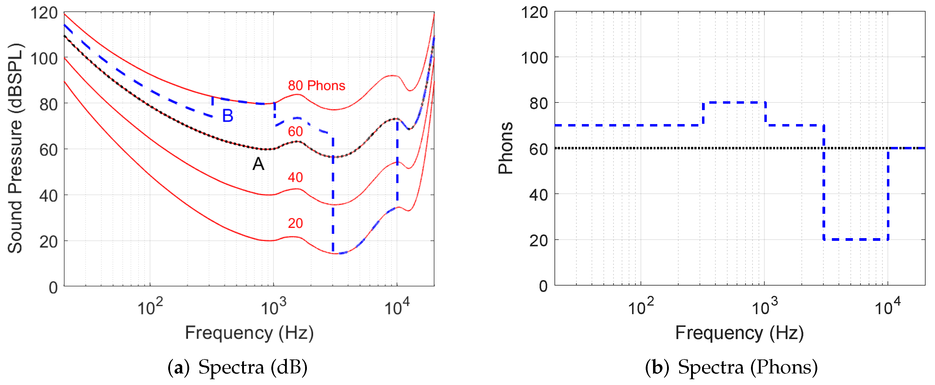
2.2. Equal Loudness Weighting

The amplitude values are weighted according to inverse equal loudness contours using the ISO 226 standard [33], such that frequencies where the human auditory system is less sensitive (such as at the limits of the audible frequency spectrum) are weighted lower, and vice versa, as follows. The sound pressure level $L_p$ in Phons, with a loudness level $L_N$ in dB, for each frequency f is defined ([33] Section 4.1) as

$$L_p=\left(\frac{10}{{\alpha }_f}.{\log }_{10}{A}_f\right)-L_U+94,$$

(1)

where $L_U$ is the magnitude of the linear transfer function at 1 kHz, ${\alpha }_f$ is the perceptual loudness exponent, $T_f$ is the threshold of hearing in Phons, and

$$A_f=(4.47\times {10}^{-3})({10}^{\frac{L_N}{40}}-1.15)+{\left[\frac{{10}^{\left(\frac{T_f+L_U}{10}-9\right)}}{2.5}\right]}^{{\alpha }_f}.$$

(2)

ISO 226 defines a series of equal loudness curves that vary according to absolute reference volume as well as frequency (see Figure 3 with two sample input signals A and B for illustration).

This converts the amplitude data from dB to the Phon scale and accounts for the frequency-varying sensitivity of human hearing, where the most sensitive frequency range is between approximately 1 kHz and 5 kHz. The approach used in this study differs from alternative methods, which use a single equal loudness contour filter based on the threshold of hearing [17,18], by utilising 90 magnitude-dependent equal loudness contours in 1 dB increments from 0 to 90 dB SPL, as perceived loudness at different frequencies changes with higher sound pressure levels [34]. The magnitude of each frequency bin of the input signal then determines the equal loudness contour used, through linear interpolation between the two closest contours. Note that while this method uses digital signals, ISO curves are designed for physical signals. Therefore, unless otherwise stated, the average amplitude of the reference input signal dataset is assumed to be 75 dB SPL, in line with commonly reported typical listening levels [35,36,37]. This value is configurable, however, and should be changed if the intended playback level is known, as it affects the equal loudness curves selected.

2.3. Phon to Sone Conversion

The magnitude value of each frequency bin is then converted from Phons to sones [38] using

$$\mathrm{sone}=2^{\left(\frac{\mathrm{Phon}-40}{10}\right)}.$$

(3)

This conversion is illustrated in Figure 4. The sone scale is based on human perception of loudness. It is well known that at normal listening levels, a drop of 10 Phons (10 dB at 1 KHz) is roughly equal to a 50% reduction in perceived loudness [12]. As the sone scale is based on human perception of loudness using the approximate ratio of +10 Phons per doubling of perceived loudness [13,39], this therefore accounts for human auditory system features such as spectral peaks being more perceptually significant than notches [40], and louder sounds carrying greater relative importance [34]. When perceiving elevation, the louder signal of the two ears (usually from the ipsilateral side) is therefore weighted with higher relevance [30], which may also be relevant for colouration perception too.

2.4. Equivalent Rectangular Bandwidth Weighting

While the FFT operation samples a time-domain signal at linearly spaced frequency intervals, the spacing of human cochlear best-frequency is approximately logarithmic. Therefore, in the PBC method the magnitude value of each frequency bin is weighted according to its equivalent rectangular bandwidth (ERB) [41] using

$${\mathrm{BW}}_{\mathrm{ERB}}=24.7(4.37\times {10}^{-3}·f_c+1),$$

(4)

where $f_c$ is the centre frequency and the amplitude value of each frequency bin is then weighted by ${\mathrm{BW}}_{\mathrm{ERB}}^{-1}$, such that the relative weight of high frequencies is reduced. This is similar to the use of a gammatone filterbank. The weighted sampling is demonstrated in Figure 5.

The colouration output value is the weighted average and is representative of the average perceptual difference in sones between the two input set spectra. A single value of PBC between each input signal in the test and reference sets is calculated as the mean difference between the weighted amplitude values of each frequency bin. The PBC of a binaural signal can then calculated as the mean of the left and right PBC values.

3. Validation

To validate the proposed method, PBC was compared to three other calculations that are used as a measure of colouration: basic spectral difference (BSD), Perceptual Evaluation of Audio Quality (PEAQ) [19], and Composite Loudness Level (CLL) [24]. These methods were chosen due to the public availability of the implementations, and because they have been widely used in binaural audio research. The first validation approach used a set of test impulses, designed with notch and peak filters at frequencies and amplitudes chosen to test the features of the method in isolation. In the second approach, a listening test was conducted on the perceived difference of degraded binaural signals, and the correlation between the perceptual results and numerical results obtained using the four tested methods was measured.

BSD was calculated as the mean value of the difference between the magnitude values of every frequency bin in the FFT calculation. PEAQ calculations used the Matlab implementation in [42] (https://github.com/NikolajAndersson/PEAQ, accessed 16 December 2021), which is the ‘basic’ version of the model [19]. CLL calculations used the Matlab implementation from [24] (www.acoustics.hut.fi/-ville/software/auditorymodel/, accessed 12 February 2020), with the middle-ear modelling and half-wave rectification from the HUT ear 2.0 package [43] and the Karjalainen1996 preset, based on research in [25]. For all methods, when using stereo signals, a single ‘binaural’ output value was calculated as the mean of the left and right values. The sampling frequency of all signals was 48 kHz.

3.1. Test Scenarios

Four scenarios of test signals were created by convolving a flat frequency response impulse with filters specifically designed to assess three features of the method in isolation. In each scenario, the calculated filters were applied to one second of stereo pink noise. For each tested feature and colouration method, the colouration value was calculated between the reference, which was the non-filtered noise, and the test signal, which was the filtered noise.

3.1.1. Feature 1: Equal Loudness

To demonstrate the use of ISO 226 equal loudness curves, two signals with +20 dB peaks at 3 kHz and 10 kHz at 65 dB SPL were compared to flat response reference signals of the same level (see Figure 6 and

Table 1. Calculated colouration values between 3 kHz and 10 kHz +20 dB peak filtered signals and flat response reference signals at the same level. Both filtered test signals used an equal filter bandwidth at 65 dB SPL.

Feature	3 kHz	10 kHz
BSD (dB)	0.48	1.01
PEAQ (ODG)	0.86	0.71
CLL (Phons)	0.62	0.48
PBC (sones)	1.12	0.26

). Both filtered test signals used an equal filter bandwidth at 65 dB SPL. The same filter was applied to both left and right channels. As the human auditory system is more sensitive to 3 kHz than 10 kHz (see again the equal loudness curves in Figure 3a), a higher value of colouration is expected at the 3 kHz signal. This is shown by the PEAQ, CLL, and PBC values, but not by the BSD. The three other methods therefore produce a result more in line with perceptual expectations in this scenario.

3.1.2. Feature 2: Binaural Loudness Difference

Second, to demonstrate the conversion from the Phon to sone scale, which is used in this method to give a greater weight to louder sounds, two comparisons were made. The first assessed how a change in loudness at a lower amplitude should be less perceptually noticeable than one at a higher amplitude, a feature highly relevant in binaural signals with interaural level differences. In this scenario, the reference was a stereo signal with a flat response at 65 dB SPL (left ear) and 45 dB SPL (right ear). The first test signal had a 1 kHz +20 dB peak on the left ear signal and an unchanged right ear signal, and the second test signal had a 1 kHz +20 dB peak on the right ear signal (20 dB quieter) and an unchanged left ear signal. An illustration of the filters is shown in Figure 7 and calculated colouration values between the test signals and flat response reference signals are presented in

Table 2. Calculated colouration values between 1 kHz +20 dB peak filtered signals at 65 dB SPL and 45 dB SPL and flat response signals of the same respective levels.

Feature	65 dB	45 dB
BSD (dB)	0.07	0.07
PEAQ (ODG)	0.19	0.19
CLL (Phons)	0.39	0.13
PBC (sones)	0.46	0.11

.

The BSD and PEAQ values are equal, regardless of whether the peak occurs on the louder or quieter side of the stereo signals. The CLL and PBC produce greater colouration values for the signal with a peak on the louder left ear signal. Due to the louder amplitudes, these signals have a higher perceptual relevance [30], so the CLL and PBC values are more in line with perceptual expectations.

The second comparison looked at the colouration values of peaks and notches by comparing signals with a 1 kHz +20 dB peak and −20 dB notch at 65 dB SPL to flat response signals at the same level (see Figure 8 and

Table 3. Calculated colouration values between 1 kHz +20 dB peak and 1 kHz −20 dB notch filtered signals at 65 dB SPL and flat response signals of the same level.

Feature	Peak	Notch
BSD (dB)	0.15	0.15
PEAQ (ODG)	1.08	0.95
CLL (Phons)	0.50	0.43
PBC (sones)	0.91	0.63

). The same filter was applied to both left and right channels.

The BSD calculation produces the same value of colouration and PEAQ and CLL give similar values, whereas the PBC method produces a value in line with what is expected from the human auditory system; a greater value for the peak than the notch, as peaks are more noticeable than notches [40].

3.1.3. Feature 3: Non-Linear Frequency Scaling

The third test scenario aimed to demonstrate the use of ERB weighting, which compensates for the linear frequency interval sampling of an FFT. To test this, two signals with +20 dB peaks at 1 kHz and 5.5 kHz, both with fixed 100 Hz −3 dB filter bandwidth, at 65 dB SPL level, were compared to flat response signals at the same level (see Figure 9 and

Table 4. Calculated colouration values between 1 kHz and 5.5 kHz +20 dB peak filtered signals with 100 Hz −3 dB filter bandwidths and flat response signals of the same level.

Feature	1 kHz	5.5 kHz
BSD (dB)	0.15	0.15
PEAQ (ODG)	1.08	0.27
CLL (Phons)	0.50	0.15
PBC (sones)	0.91	0.12

). The frequencies of 1 kHz and 5.5 kHz were chosen as these are frequencies at which the ear has approximately the same sensitivity. The same filter was applied to both left and right channels.

Again, the BSD calculation produced the same result for each signal, whereas the PEAQ, CLL, and PBC produced values that are more in line with perceptual expectations: a greater value of colouration for the peak with a wider perceptual bandwidth.

3.2. Listening Test

The second way in which the PBC method validated was to assess the correlation between colouration calculations and human perception of spectral similarity. To achieve this, a listening test was conducted with varying levels of spectral degradation of the binaural signal. The results of the test were compared to different colouration calculation methods for correlation. The four tested methods in the comparison are BSD, CLL, PEAQ, and PBC.

Listening tests were conducted on 9 participants aged between 24 and 43 with a median age of 31 and self-reported normal hearing. All were considered experienced listeners and had participated in multiple previous listening studies. Tests were conducted at home offices, due to the Covid-19 pandemic, with Sennheiser DT-990 Pro headphones and Focusrite Scarlett Solo audio interfaces.

A single equalisation filter for all headphone sets was used, equalised using 10 measurements of 10 different headphone sets obtained from a Neumann KU 100 dummy head using the exponential swept sine impulse response technique [44] and re-fitting of the headphones between each measurement. Equalisation filters were calculated from the RMS average of the 100 deconvolved headphone transfer functions (HpTFs) using Kirkeby and Nelson’s least mean square regularisation method [45], with one octave smoothing implemented using the complex smoothing approach of [46] and a range of inversion 5 Hz–4 kHz. In-band and out-band regularization of 25 dB and −2 dB, respectively, was used, chosen to reduce sharp peaks in the inverse filters.

3.2.1. Test Paradigm

The listening test followed the MUSHRA paradigm, ITU-R BS.1534-3 [47], using webMUSHRA [48] (https://github.com/audiolabs/webMUSHRA, accessed 16 December 2021). The base stimulus was one second of monophonic pink noise at a sample rate of 48 kHz, windowed by onset and offset half-Hanning ramps of 5 ms. Each test sound was first generated by convolving the pink noise with HRTFs from the Bernschütz Neumann KU 100 database [49]. The test sound locations ($\psi$) of the HRTFs corresponded to the central points of the faces of a dodecahedron. To reduce the total number of trials, symmetry was assumed and thus only locations in the left hemisphere were used, amounting to 8 locations (see

Table 5. Spherical coordinates of test sound locations, corresponding to the central points of the left hemispherical faces of a dodecahedron.

$\mathit{\psi }$	1	2	3	4	5	6	7	8
$\theta$ (°)	180	50	118	0	180	62	130	0
$\varphi$ (°)	64	46	16	0	0	−16	−46	−64

). All binaural renders were static (fixed head orientation) to ensure consistency in the experience between participants. Low anchor and medium anchors were low-pass filtered versions of the reference with an $f_c$ of 3.5 kHz and 7 kHz, respectively.

For each test sound location, the conditions were degraded versions of the reference created using a 10-band filter stage in one octave bandwidths from 31.5 Hz to 16 kHz, with centre and edge band frequencies as in the ANSI standard S1.11-2004. The gain of each octave band filter was calculated as $R{g}_{\mathrm{EQ}}$, where R is a uniformly distributed random number that follows $R=\mathbb{R}$, $R\in (-0.5,0.5)$, and $g_{\mathrm{EQ}}$ is the equaliser gain. Filters were generated separately for left and right ears in order to increase the binaural differences between conditions, such that some conditions would have larger gains in certain frequency bands in the ipsilateral signal, and some in the contralateral. For each test sound location, seven test conditions were generated using equaliser gains $g_{\mathrm{EQ}}=\{1,2,4,6,8,12,16\}$, totalling 7 conditions per test sound location, and therefore 56 in total. An illustration of the 10-band equaliser with varying equaliser gains (for one ear) is presented in Figure 10. Equaliser curves were applied to the binaural pink noise signals.

For each trial, the listener was asked to rate the stimuli in terms of similarity to the reference. The presentation of stimuli and trials was randomised and double blind, and participants were able to adjust the playback level at the start of the test, after which it was fixed.

3.2.2. Results

Values of colouration were calculated between the test and reference stimuli. To compare the perceptual results from the listening test to those of the four colouration methods, the mean perceived similarity ratings of each condition are plotted against the corresponding colouration values from the four tested methods in Figure 11. Results for each test sound location (see again Table 5) are presented in different colours, and a linear regression is denoted by a black line. Reference and anchor results were omitted. The Pearson’s correlation coefficient, between the mean listening test results for each condition and the colouration results for the four tested methods, is presented in

Table 6. Pearson’s correlation coefficient results comparing the mean MUSHRA test results to the four colouration calculations of the test stimuli and the references, over all test sound locations.

Correlation	r	p
BSD	−0.83	<0.001
PEAQ	−0.52	<0.001
CLL	−0.90	<0.001
PBC	−0.95	<0.001

.

All four tested methods produced a statistically significant (p < 0.001) negative correlation between colouration values and perceived similarity. Negative correlation values are expected as the comparison is between a measure of similarity (perceived similarity) and a measure of difference (colouration). However, the PBC method produces the highest value of correlation ($r=-0.95$), and this is reflected in Figure 11 by the small distance between the individual points and the linear regression. CLL has the second highest correlation, at $r=-0.90$, followed by BSD, and finally PEAQ.

To assess how the colouration calculations perform at different directions,

Table 7. Pearson’s correlation coefficient results comparing the mean MUSHRA test results to the four colouration calculations of the test stimuli and the references, for each test sound location as in Table 5.

$\mathit{\psi }$	1	2	3	4	5	6	7	8
r (BSD)	−0.96	−0.98	−0.90	−0.97	−0.93	−0.96	−0.98	−0.71
r (PEAQ)	−0.87	−0.24	−0.39	−0.85	−0.96	−0.50	−0.21	−0.20
r (CLL)	−0.97	−0.96	−0.96	−0.95	−0.99	−0.94	−0.98	−0.92
r (PBC)	−0.99	−0.99	−0.95	−0.99	−0.99	−0.98	−0.98	−0.97
p (BSD)	<0.001	<0.001	0.006	<0.001	0.002	<0.001	<0.001	0.073
p (PEAQ)	0.010	0.600	0.386	0.016	<0.001	0.247	0.651	0.667
p (CLL)	<0.001	<0.001	<0.001	<0.001	<0.001	0.002	<0.001	0.004
p (PBC)	<0.001	<0.001	0.001	<0.001	<0.001	<0.001	<0.001	<0.001

presents the correlation between the listening test results and the colouration calculations for each test sound location (see again Table 5). Reference and anchor results were omitted.

The CLL and PBC all produced a high negative correlation for all test sound locations ($r<-0.90$). The BSD produced high negative correlation for most locations ($r\le -0.90$), with the exception of $\psi =8$ ($r=-0.71$), corresponding to $(\theta ,\varphi )$ = (0°,−64°). The PBC produced very high correlation values for all test sound locations ($r\le -0.95$), and was the highest out of the four tested colouration calculations for all test sound locations except $\psi =3$, corresponding to $(\theta ,\varphi )$ = (118°,16°), where CLL produced a higher negative correlation value ($r=-0.96$ and $r=-0.95$).

3.3. Discussion

The PBC method performed comparably with three alternative publicly available and widely used methods as an objective prediction of the colouration between binaural signals. This was shown first with specific test scenarios, intended to isolate the features of the method, for which the presented method produced colouration values that fit with expectations.

Second, the correlation between the subjective results of a listening test conducted on perceived similarity of binaural signals and the colouration values of the four tested methods was measured. All four tested methods produced a statistically significant ($p<0.001$) overall negative correlation between colouration values and perceived similarity, though the presented PBC method produced the highest overall correlation value ($r=-0.95$), which is notably higher than the other tested methods. One reason for this could be the sone loudness scale, allowing for a greater perceptual weight for louder frequency bands.

Further analysis on specific test sound locations showed that the PBC produced the highest correlation values for all but one tested sound location, and the correlation plots in Figure 11 show the PBC as consistently producing a colouration result close to the linear regression line. However, the BSD, CLL, and PBC values are less correlated with the listening test results at lower levels of signal similarity, which could be an avenue for further work.

The validation has shown that the PBC method for predicting the colouration between binaural signals correlates highly with the perceptual results of a listening test on similarity. These are the highest correlation values out of the four colouration calculations tested. However, other relevant methods of predicting colouration exist that were not included in this study due to the availability of source code, and should be included in further validation [50,51]. Additionally, further validations could utilise a wider range of test stimuli, with impulsive noises such as click trains, tonal noises such as sine waves, as well as real-world sounds with greater dynamic ranges, such as speech and music. Note that the number of participants in the listening test was limited by COVID-19 regulations. Further validation should aim for more participants with a greater diversity; nonetheless, the results with the current number of participants is sufficient to conclude that the presented method is highly correlated with the listening test results.

4. Conclusions

This paper has presented a loudness method for predicting the perceived colouration between binaural signals using perceptually motivated signal processing techniques prior to the difference calculation. Applications of the method include testing of prototype binaural reproduction systems, such as those used in virtual and augmented reality, to reduce the need for conducting time-consuming and resource intensive perceptual listening tests.

The method has been validated by comparison to a basic spectral difference and two alternative publicly available methods that are used to predict colouration. The predicted binaural colouration method produces results in line with expectations from the literature, which formed the motivations of the calculation, and correlates highly with results from a perceptual listening test, with correlation values that are higher than the other tested methods. This suggests the method is appropriate for predicting the colouration between binaural signals.

Though the presented method correlates well with perceptual listening in the tested scenario, the current validation is somewhat limited. Further validation is necessary using other published methods and stimuli with greater temporal and dynamical differences. Future development in binaural colouration modelling should also incorporate modern neural-network based human cochlear models [52] as well as elevation-specific perceptual cues [30].

The predicted binaural colouration method is implemented as Matlab code in the publicly available Auditory Modeling Toolbox, version 1.0 (https://www.amtoolbox.org/, accessed 16 December 2021), under the name mckenzie2021.