The Historical Transformation of Peri-Urban Land Use Patterns, via Landscape GIS-Based Analysis and Landscape Metrics, in the Vesuvius Area

Abstract

Peri-urban areas constitute an enormous resource in terms of natural capital, landscape heritage and economic activities, but, at the same time, they are often affected by physical and socio-economic degradation, drawing the attention of decision makers and planners. Many studies have focused on these contexts both in terms of suburbs, with a close dependence on urban centers, and new land typologies. The present paper focuses on documentary evidence of the direct impacts of urban growth on rural lands. The study area entails the Vesuvius National Park, which, belonging the Naples metropolis, is well-known for its historical, geo-morphologic and naturalistic value. Furthermore, the area has a history of high-quality cartographic production: the 1817, 1907, 1960, 2009 time steps maps were digitized, georeferenced, vectorized and compared in a GIS environment. The results highlight a strong change in land-use, in vineyards and urban class types, with a more disaggregated landscape mosaic. The approach shows that the historical modeling of land-use changes supports the understanding of current land-use dynamics and landscape patterns. The study also shows the need to integrate landscape planning and landscape ecology approaches, highlighting the close interactions between urban, agricultural and natural areas, for the purpose of supporting decision makers in land-use management and conservation policies.

1. Introduction

Agro-forest land constitutes an enormous resource in terms of natural capital and cultural heritage, in addition to the economic/productive potentialities connected with primary sector activities. However, at the same time, these areas demonstrate a highly transformable character, due to their limited physical inertia, moderate transformation costs and position factors. The urban growth is considered one of the most important driving forces in shaping landscapes, with direct and strong long-term impacts on agro-forest land, with this decreasing with the distance from the urban centres [1]. Thus, within the main type of agro-forest lands, peri-urban areas hold an especially fragile and vulnerable status, as they still have a high potential for transformability, due to the close physical, functional and perceptive relationship with urban areas, which represent the most extreme expression of the anthropogenic transformation of the environment.

The unstable nature of peri-urban areas makes them particularly susceptible to problems and critical issues; among them, physical and social marginality (the suburbs) is undoubtedly a constant issue, with important repercussions in terms of the productivity, safety and quality of the environment. This phenomenon is particularly dramatic in large urban and metropolitan areas; however, degradation phenomena in peripheral areas also involve medium and small urban areas, drawing the attention of decision makers and planners. Many studies have focused their research on sub-urban contexts, precisely because these are the stage for many contemporary social, economic and political issues [2]. On the one hand, peri-urban contexts are considered suburbs, highlighting their close interactions with and dependence on urban centres. On the other hand, they are treated as new land typologies, considered as transitional zones between definitively urban and unequivocally rural areas, with them being referenced to in several ways, namely as rural-urban fringes/transition zones or zones/areas of interfaces [3].

In the present work, according to these new land typologies, urban peripheries were studied in terms of the evolution of the physical relationship between urban and peri-urban areas and between urban and peri-urban areas in terms of land use, by means of the land use/cover change (LUCC) analysis. LUCC is a key topic for environmental scientists, being the process by which human activities transform the landscape (from natural vegetation to any other uses). LUCC often causes environmental problems, such as global warming, habitat loss and fragmentation, the alteration of biogeochemical cycles, soil erosion, which is responsible for devastating effects on biodiversity and, in terms of a longer perspective, human well-being [4,5,6,7,8]. Therefore, the study of LUCC, in terms of both historical and prediction analysis, can help decision-makers and scientists to achieve:

• a better understanding of the current state (land composition and conformation) of land systems;
• the identification of the dynamics of and driving forces behind complex systems in a territorial context;
• the monitoring of these dynamics;
• the evaluation of adopted strategies and policies;
• the construction of future scenarios and the assessment of their possible environmental and socio-economic impacts;
• the support of the land management and planning, according to sustainability principles.

When it comes to historical LUCC, historical maps are effective sources of geographical information and are useful for historical and territorial research. The availability of chronological historical maps makes it possible to conduct multi-temporal studies and analysis on landscape changes [9], especially in terms of landscape coverage, for the purpose of supporting landscape planning and management in the present and the future. Generally, in terms of representation and contents, the time steps investigated span about one century, due to the difficulty of gathering reliable and accurate historical cartographies.

The area surrounding Vesuvius in the Campania region in southern Italy constitutes an exception in this sense due to the production high-quality cartographic records which date back to the end of the seventeenth century. This area is therefore useful in terms of providing a reference for in-depth studies on historical cartography and as a basis for macro-analysis about land use/cover dynamics. The analysis of historical LUCC with the support of GIS technologies allows for the highlighting of not only what has changed, that is, variations in the surfaces of various classes of land use, but also the structure/composition and configuration of these variations.

The landscape ecology approach, which integrates ecology and physical geography principles and both uses landscape metrics as tools for analysis and quantifies landscape proprieties, is an important tool in such contexts. The study of landscape composition and configuration, targeted on the specific issue of urban/peri-urban dichotomy, can contribute to knowledge of the landscape (and its development) and can help to develop strategies for the mitigation of the negative conditions in many urban surroundings areas. Landscape metrics (LMs) are algorithms which, quantifying the spatial characteristics of patches, classes of patches or entire landscape mosaics, help to mathematically assess landscape structure and can give valuable information to improve the assessment of the ecological functioning, economic wealth and aesthetic value of a region [10,11]. Numerous landscape metrics have been developed, depending on the objectives of the study or the survey scale. Gustafson [12] divided them into two broad categories, those that quantify the composition (presence, relative abundance or diversity of landscape types) and those that quantify the spatial configuration of the landscape (spatial distribution and form). Mc Garigal [13,14] organized them at different scale levels (patch level, class level and landscape level), which correspond to a logical hierarchical organization of spatial heterogeneity in patch mosaics and in terms of types (area and edge; shape; core areas; contrast; aggregation; diversity). Many studies have used landscape metrics to analyse the spatial characteristics of urban growth [15,16,17,18], mainly focusing on large-size/metropolitan cities and on US contexts. Therefore, more insights are required with regard to Mediterranean cities. In this context, not only large urban areas, but also medium-sized cities are characterized by specific morphological and historical features, and, at the same time, more recently, by dramatic changes which not always in continuity and dialogue with the existing urban fabric.

Taking a previous study on land use change in the Vesuvius area [19] as a starting point, in the present paper, the specific issue of the development of peri-urban areas was studied more deeply. A territorial scale analysis was performed, rather than an urban morphology one. This study of land use, specifically with respect to the relationship between urban and peri-urban areas, as well as its high level of analysis, allows for a better understanding of development guidelines and territorial balances by relating them to other physical elements present in the landscape: roads, productive or commercial districts, urban areas, etc. The work entails two sections. The first one focuses on historical cartography and the study of land use/cover changes. Historical maps of the “Regno di Napoli” (Naples Kingdom) were processed by means of GIS support techniques. The second section is devoted to landscape analysis, by means of defined landscape metrics, in order to deepen our understanding of the relationship between urban and infrastructural areas and their surrounding areas.

The results show that the area was subject to dramatic changes in land use. Major changes were registered in vineyards and urban class types (about −99.6% and +670%, respectively). Furthermore, landscape mosaics now appear more disaggregated due to different numbers of patches and their more irregular shapes.

Thanks to the available cartographic data, this work aimed to investigate what has happened and changes in land uses types in the Vesuvius context over the last two centuries due to geo-genic or anthropogenic factors which have significantly transformed this area. The study area is under strong anthropic pressure, but, at the same time, also has a high environmental value (witnessed by the presence of one national park, two sites of community importance and one special protection area) and a well-known cultural heritage, including the traditional landscape, which has to be preserved but also improved. Starting from a specific case-study, the general aim of the paper was to implement a framework of action via landscape analysis to support the activity decision-makers. The study shows the usefulness of integrating landscape planning and landscape ecology approaches, highlighting the close interactions between urban, agricultural and natural areas, with the aim of contributing to our knowledge of, as well as the prevention, mitigation and/or combating of, the phenomena of the physical, but also often the social, degradation of agro-forest areas, especially in peri-urban areas.

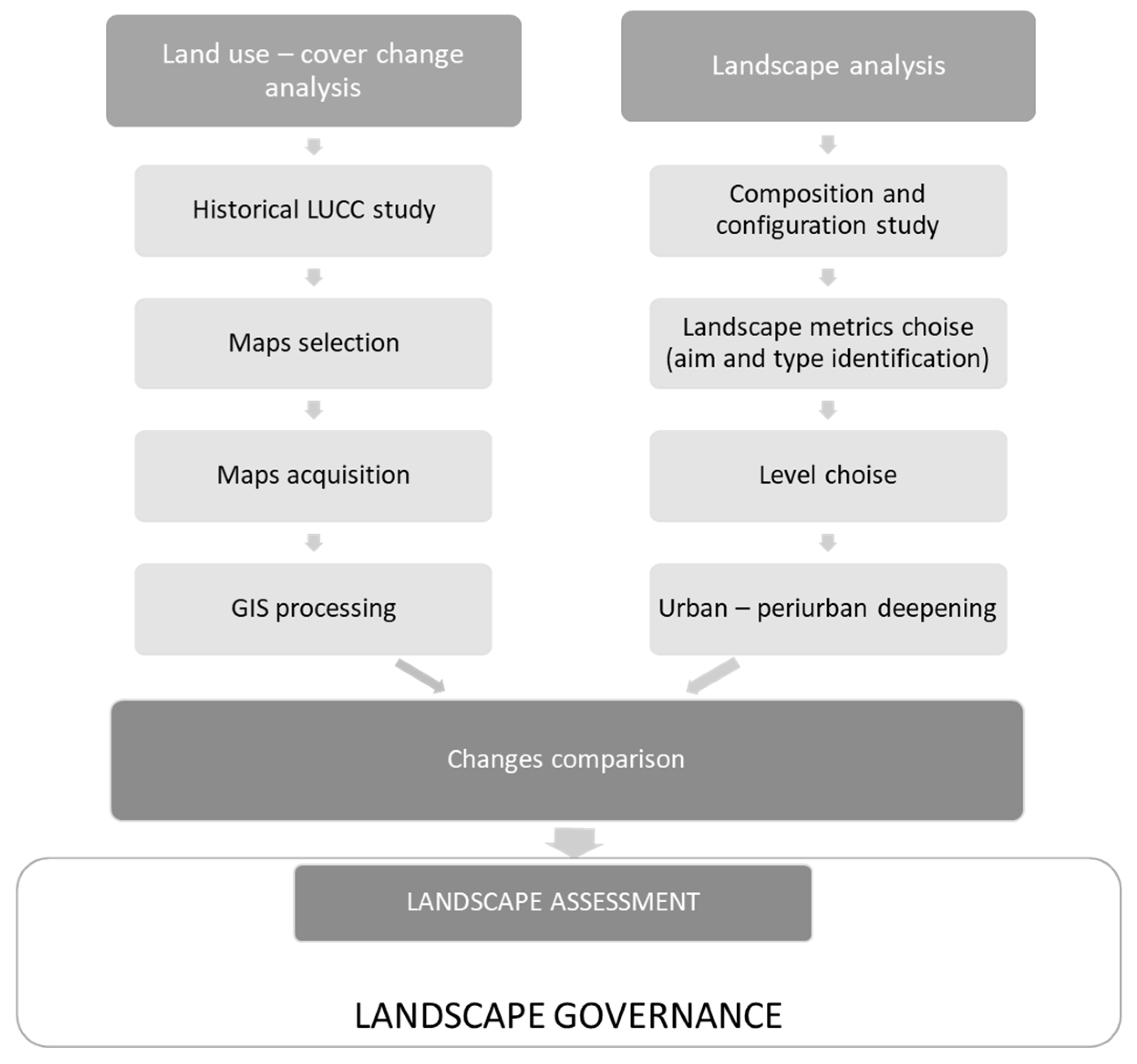
2. Materials and Methods

The paper comprises two main sections (Figure 1): land use/cover changes analysis and landscape analysis. Their integration is aimed to support land governance.

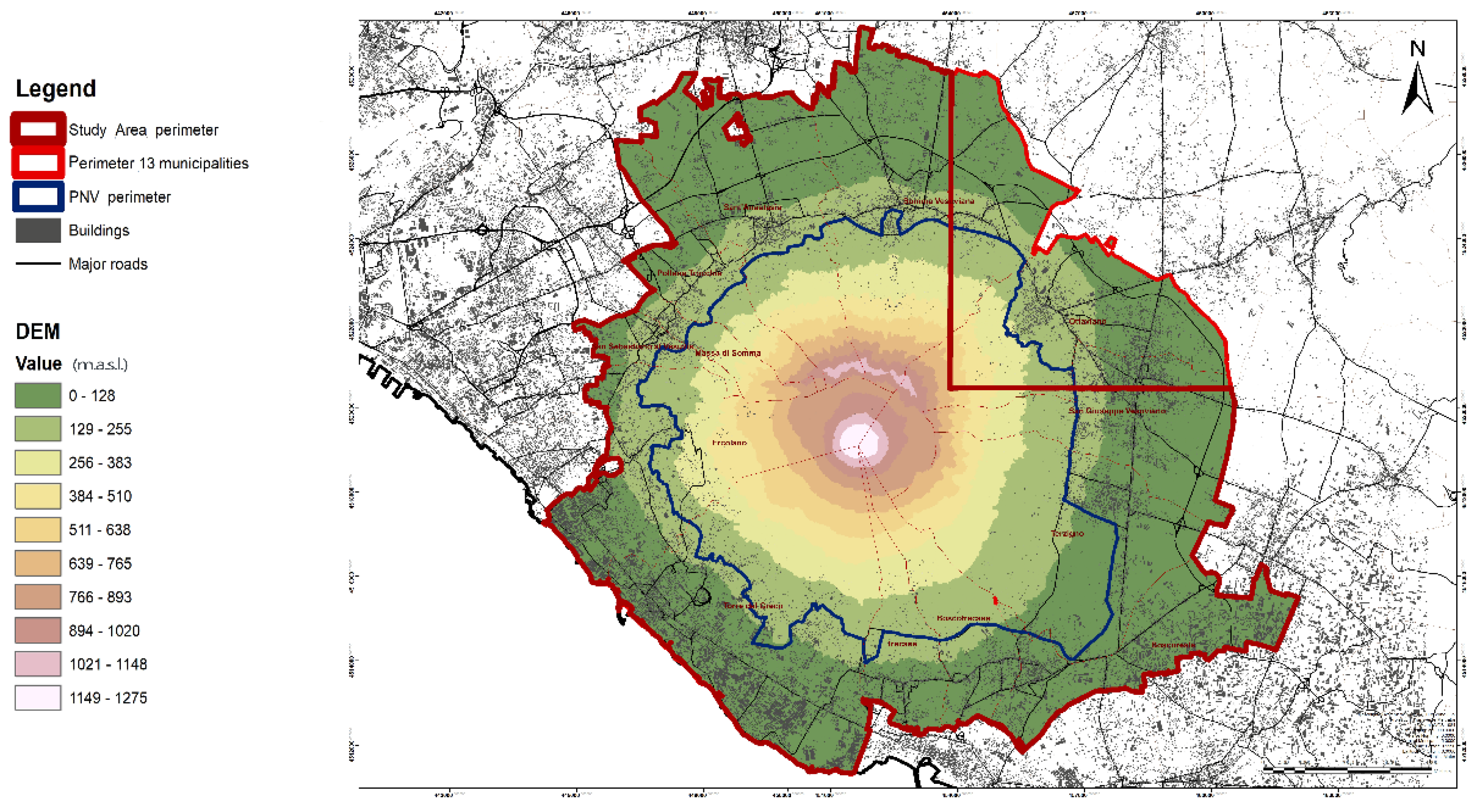
2.1. The Study Area

The study area boundaries were delimited based on the availability of historical maps, with the aim of including areas with both urban and extra-urban land use types. Specifically, the work focuses on an area that begins on the outer limits of the Vesuvius National Park, which includes the areas closest to the cone, which are not directly urbanized ad are inserted in a context of strong anthropization (the metropolitan area of Naples includes three million of inhabitants). For the purposes of the study, it was considered useful to include in the study area the entire territory of the 13 municipalities belonging to the park in order to allow for the assessment of the context of rural and man-made dynamics. A further step was necessary when it came to defining the area under study due to the availability of historical data and maps: Sheet 185 IV-SW (S. Giuseppe Vesuviano), belonging to the old 1906 series, is not available from the Geographic Military Institute (GMI) archives. The need to make a comparison between different temporal steps forced us to remove the part of the territory of the Ottaviano and Somma Vesuviana municipalities belonging to the missing sheet.

The final study area extends to 19,565 ha (Figure 2). The altitude ranges from sea level to 1275 m.a.s.l. The study area includes the still active “Somma-Vesuvius” volcanic complex, the most important volcano in continental Europe. The archive/database of the historical eruptions of Vesuvius [20] is very interesting for the purposes of this work, as it allowed us to relate LUCC with geogenic factors. The database reports as many as 13 eruptions between 1817 and 1907, which justify the spatial extent of the areas covered by ashes. In particular, the eruption of 1906 is known as the most violent manifestation of the activity of Vesuvius in the 1900s. There were only two eruptions between 1907 and 1960, but the 1944 one was particularly violent, with ashes that reached the Adriatic side of the Peninsula.

From the naturalistic point of view, the two sides, the Vesuvian side and that of the Somma Mountain, respectively, are different: the Vesuvian side is more arid and is largely reforested to prevent landslides, presenting the typical vegetation of Mediterranean scrub. The Somma Mountain is wetter and is characterized by the presence of mixed woods.

The 13 municipalities have a population of 310,531 inhabitants (2011 census data). Analysis of the population trend over the whole last two centuries shows a general increase in inhabitants, with a higher rate during the period of 1911–1961 (Figure 3).

Since World War II, the surrounding areas of the National Park have seen progressive landscape saturation due to the building of new infrastructure and industrial settlements as a consequence of urban growth.

Nevertheless, since the establishment of the Vesuvius National Park in 1995, the natural protected area has had a rich historical and naturalistic heritage, with an agricultural production that is unique in its variety and originality of flavours. The main agri-food products, also underlined by quality food certifications, have their strengths in wine, apricots and tomatoes.

2.2. Land Use/Cover Change Analysis

2.2.1. Historical Maps Acquisition and Recent Dataset Analysis

Different time steps were processed, starting from historical maps up to recent maps, covering the last two centuries. The maps are:

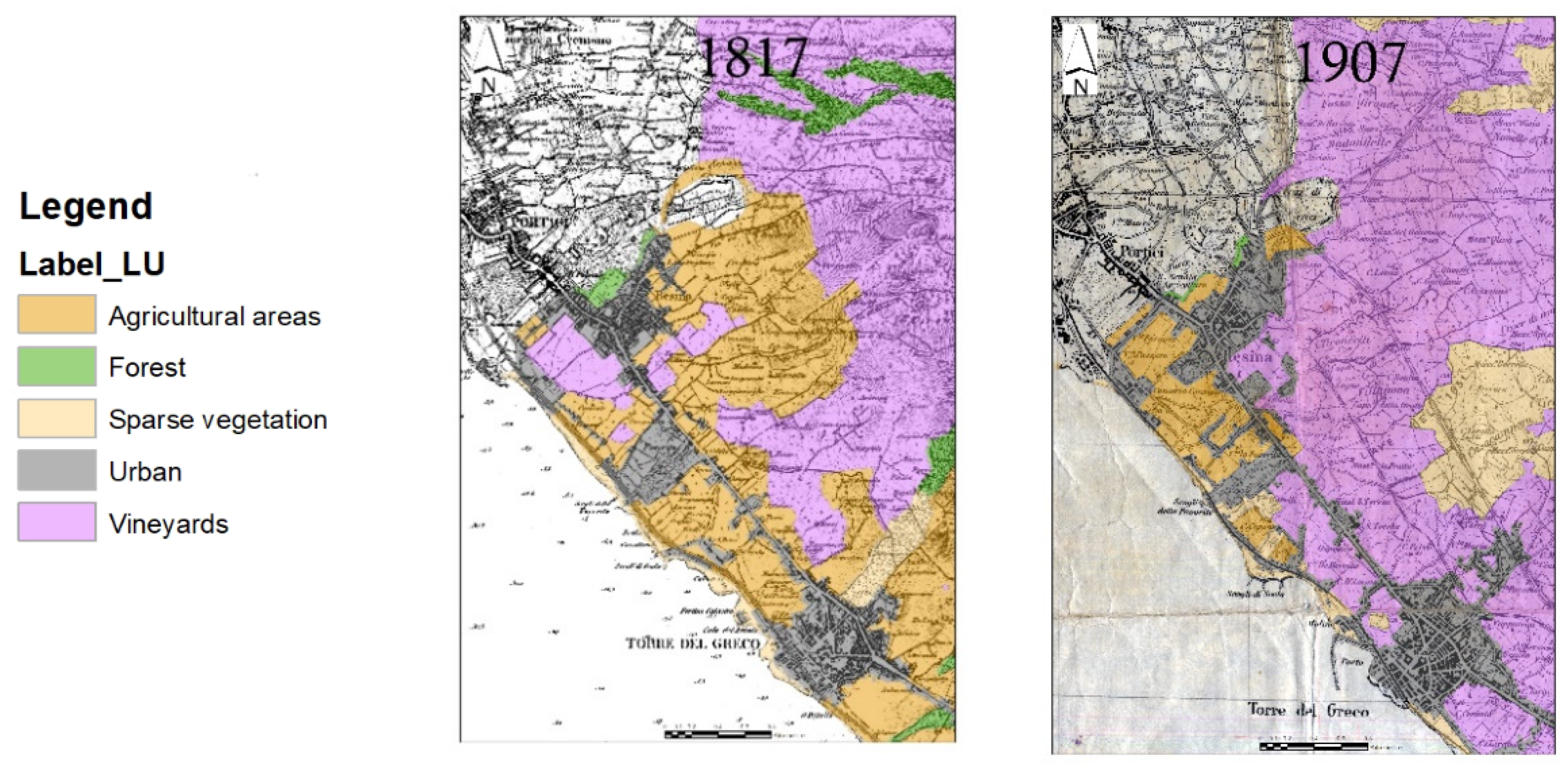
• 1817—Topographic and hydrographic map of the contours of Naples (Topographical Office of the Naples Kingdom)—1:250,000. The accuracy of the map and its history was reported by Pindozzi et al. (2016)
• 1907—Topographic map of Italy series 25v (Military Geographic Institute)—1:25,000
• 1960—Land use map of Italy (National Research Council and Italian Touring Club)—1:200,000
• 2009—Campania region agricultural land uses map (Agricultural Division of the Campania Region)—1:50,000

To support the geo-referencing of historical maps, Regional Technical Cartography (CTR) 2004–2005, scale 1:5000, was used.

• 1817—Topographic and hydrographic map of the contours of Naples (Topographical Office of the Naples Kingdom)

In the present work, the map sheets were acquired, in digital and paper formats, from the archives of the University of Naples Federico II. For the specific study, sheets 9 and 12 were used.

• 1907—Topographic map of Italy series 25v (Military Geographic Institute)

The map of Italy drawn up by the Military Geographic Institute (MGI) is the official Italian topographic map, produced in three different scales: 1:100,000, 1:50,000 and 1:25,000. The symbology used for land use classes was unchanged over the years. This “coherence” of representation makes it possible to evaluate, both in qualitative–quantitative and in synchronic–diachronic terms, the different types of land use destinations [9,21]. For the purpose of the present work, the topographic map used belonged to the so-called “first survey” (prima levata) of 1907. These maps were created based on an initial survey conducted during the years 1875–1876, which was updated only for specific aspects (i.e., new roads, reclaimed areas, etc.). For this reason, even though they have documentary value, these maps do not provide an exhaustive description of an area. In the present work, the sheets 184 I-SE (Pomigliano d’Arco), 184 II-NE (Monte Vesuvio) and 185 III-NW (Boscotrecase), all at a scale of 1:25,000, were used and surveyed exclusively using the topographical method. The cartography was acquired in digital format from the Italian Military Geographical Institute. The absence of the sheet 185 IV-SW (S. Giuseppe Vesuviano) in the MGI’s archives affected the boundaries of the study area.

• 1960—Land use map of Italy (National Research Council and Italian Touring Club)

The land use map of 1960, from the NRC and TCI, is the first thematic document on the theme of land uses produced in Italy at the national scale [9,22]. In the present work, sheet 16 was used. The thematic map was acquired from the Geography Library Unit of the University of Naples Federico II. The hard copy was scanned at 300 dpi.

• 2009—Campania Region Agricultural land uses Map

In the present work, the land use map of 2009 was used. This map of agricultural land use (ALUM) of the Campania region was produced by the Department of Agriculture of the Campania region. The map was produced at the scale of 1: 50,000, in digital format, obtained from data at a scale of 1:25,000 and in the WGS1984 UTM Zone33N reference system.

2.2.2. GIS Processing

To trace the processes of peri-urban development over the years in the study area, the cartographic documentation, covering about two hundred years, was analysed. As a first step, the hard copies of the maps were scanned as raster files in TIFF format at 300 dpi resolution. Then, the raster datasets were imported into ArcMap of ESRI^® for the georeferencing process, which results into a coordinate transformation algorithm; a first order polynomial was used. The algorithm links the scanned historical map to the current reference projection system (UTM-WGS84, zone 33 N [23]. In order to associate the historic maps with a common geo-referencing system, the ground control points (GCPs) method was used (ArcMAP georeferencig tool), basing on georeferenced topographic regional maps (TRM, 2004–2005). This method consists of establishing a mathematical/statistical relationship between the coordinates of the pixels on the acquired raster map and those of the reference map by means of a set of ground control points (GCPs). The number of GCPs used was high enough to achieve a satisfactory level of transformation accuracy. The average root mean square (RMS) value was calculated for each map, and the associated error to the transformation was obtained by the link table in the ESRI ArcMAP software. Then, the MapAnalyst Visual open-source Java application (Jenny and Hurni 2011) was used to assess the accuracy of the historical maps. MapAnalyst calculates the mean position error (MPE) and standard deviation (SD), obtaining the mean deviation error for all of the control points on the old maps. The MPE and SD lower values are referred to higher values in terms of the accuracy of the old maps. Data processing and georeferencing accuracy assessment are reported in Pindozzi et al., 2016 [9].

Then, historical maps of the same date were patched together with the mosaic raster tool of the ArcMap toolset. The manual vectorization procedure was preferred, because it does not require specific software and if performed accurately, it can guarantee considerable precision in terms of the interpretation of map contents. The entities were visually recognized and reconstructed according to the work of Pindozzi et al. (2016) [9]. For the two topographic maps of 1817 and 1907, the meaning of symbolism was derived by Mori [24], for instance, the label of agricultural use was generally highlighted by irregular polygons and small circles along the sides, urban areas were generally black rectangles and sparse vegetation was depicted by patchy narrow lines (Figure 4). The maps of 1960 and 2009 were thematic, so classes were visually recognized according to the attribute clearly reported on the legend. In order to perform a multi-temporal direct comparison of paired land use maps, it was necessary to apply thematic generalization [9,22,23,25]. Starting from the 1817 map labels, the classes considered were the following: agricultural use, vineyards, urban, sparse vegetation, forests and waters. The water class was omitted in the subsequent evaluation of the Vesuvian landscape, as it was not of interest within the perimeter of the study area. The choice to not combine the classes of vineyards and agricultural use was made in order not to lose the information on vineyards which has been reported with a very clear symbolism already, starting with the cartography of 1817. The symbol used for vineyards was the same in the two maps of 1817 and 1907, represented as a wavy line with a small trait on the bottom part, and it was clearly different from other type of rows of plants (Figure 4). For olive groves, the other historically widespread class of agricultural use in the area, however, it was not possible to introduce a separate class since no dedicated symbolism was found on the map sheets of 1817. The thematic generalization for the 1817, 1907 and 1960 map legends was derived by Pindozzi et al. [9]; while the thematic generalization of the 2009 map was processed according to the classification reported in

Table 1. Thematic generalization for the 2009 LU map.

Land-Use Label	Land Use Classes in the 2009 Map (Campania Region Agricultural Land Uses Map)
Urban	Urbanized environment and artificial surfaces
Agricultural areas	Protected crops (greenhouses); arable crops (autumn-winter arable crops, spring-summer arable crops, alternate fodder crops, other arable crops); permanent crops (orchards and minor fruits, fruit trees or shrubs plants, olive groves, citrus groves, fruit chestnut groves, poplar groves, willow groves, other broad-leaved trees, other permanent crops or fruit trees); permanent forage; heterogeneous agricultural areas
Vineyards	Vineyards
Forest	Deciduous woods; coniferous woods; mixed forests of conifers and deciduous trees
Sparse vegetation	Mainly shrubby and / or herbaceous vegetation cover in natural evolution (natural pasture areas and high altitude grasslands, bushes and shrubs, areas with sclerophyll vegetation, areas with arboreal and shrub vegetation in evolution, areas with natural recolonization, areas with artificial recolonization and reforestation); open areas with sparse or absent vegetation; beaches, dunes and sands, bare rocks and outcrops; areas with sparse vegetation; areas degraded by fires and other events
Water/Other	Waters; wetlands

.

In order to evaluate the evolution of peri-urban areas, and, above all, the change of the land use classes enclosed in new urban expansions, a comparative analysis was developed for each period considered (1907, 1960, 2009) between the urban boundaries of each time step and the LU map of the previous one, using the ArcGIS Clip tool. The following LU maps were created and compared in pairs:

• the land use map of 1817 within the urban boundaries of the 1907 map;
• the land use map of 1907 within the urban boundaries of the 1960 map;
• the land use map of 1960 within the urban boundaries of the 2009 map;

For the LU map of 2009, the buffer areas of the urban areas, at 100 m, were analysed.

2.3. Landscape Analysis

Land use/cover change (LUCC), as the result of policies and human activities, modifies the original structural integrity of the landscape, determining new landscape patterns and affecting the ability of ecosystems to provide the services and biodiversity on which humans definitely depend [19,26]. For these reasons, landscape ecology focuses on the analysis of landscape structure and ecological processes and their implications [27], and as such has developed the landscape metrics concept. Due to their capacity of characterizing landscape patterns basing on spatial attributes, landscape metrics can be considered as a useful tool for analysing the structure, function and dynamics of landscapes. Landscape metrics are algorithms that quantify spatial characteristics of patches, classes of patches or entire landscape mosaics, supporting landscape analysis by means of objective/mathematical indices. In these terms, they contribute to providing valuable information to improve the assessment of the ecological functioning, economic wealth and aesthetic value of a region [11,28,29]. The transformation of urban and peri-urban land use patterns is generally analysed by means of LMs in order to better understand and more accurately characterize developmental processes and their consequences, in terms of both past recognition and the assessment of constructed scenarios [30,31,32,33].

In the present paper, starting from different studies dealing with the issue of uncontrolled urban expansion [18,33,34], several LMs were chosen. The aim was to identify the urban/peri-urban spatial processes that characterized the study area, in terms of aggregation, compaction and dispersion/isolation, with reference to the each time step considered. Specifically, a small set of metrics was chosen at class level, and the four time step maps were processed. According to the Aguilera analysis method [33], developed for Mediterranean urban growth in the case of a medium size city, the selected metrics are described as follows (

Table 2. Detailed description of the set of metrics used.

Urban Growth Process	Metrics
	Acronym	Formulae	Description
Aggregation	NP	ni	NP ≥ 1 The number of patches is a simple measure of the extent of subdivision or fragmentation of the patch type. 1 = the landscape contains only one patch of the corresponding patch type, when the class consists of a single patch.
	AREA_MN	$a_{ij} \left(\frac{1}{10,000}\right)$	Area ≥ 0 This is the mean of the patch size (AREA_MN) at the class level. A reduction in AREA at class level usually indicates increasing the fragmentation of a land use/cover class.
	PLAND	$\frac{{{\displaystyle \sum }}_{j=1}^n{a}_{ij}}{\mathrm{A}}\left(100\right)$	0 < PLAND ≤ 100 The percentage of the landscape quantifies the proportional abundance of each patch type in the landscape. 0 = all patches of habitat disappeared; 100 = one habitat occupies all the landscape.
Compaction	GYRATE_MN	${\displaystyle {\displaystyle \sum }_{r=1}^z}\frac{h_{ijr}}{z}$	GYRATE ≥ 0 GYRATE equals the mean distance between each cell in the patch and the patch type centroid. Radius of gyration is a measure of patch extent; thus, it is effected by both patch size and patch compaction and can be considered a measure of the average distance an organism can move within a patch before encountering the patch boundary from a random starting point. 0 = the patch consists of a single cell. The maximum values imply the patch comprises the entire landscape.
	SHAPE_MN	$\frac{{{\displaystyle \sum }}_{j=1}^n{h}_{ij}}{ni}$	SHAPE ≥ 1 This shape index (SHAPE) measures the complexity of patch shape compared to a standard shape (square) of the same size and offers a fundamentally patch-centric perspective on the landscape structure. SHAPE equals patch perimeter (m) divided by the square root of patch area (m2), adjusted by a constant to adjust for a square standard. 1 = the patch is square and increases without limit as patch shape becomes more irregular
Dispersion	ENN_MN	hij	0-Limitless This metric relates to the distance to the nearest patch of the same land use/cover class. ENN equals the distance (m) to the nearest neighbouring patch of the same type, based on shortest edge-to-edge distance. 0 = the distance to the nearest neighbour decreases. The upper limit is constrained by the extent of the landscape.

):

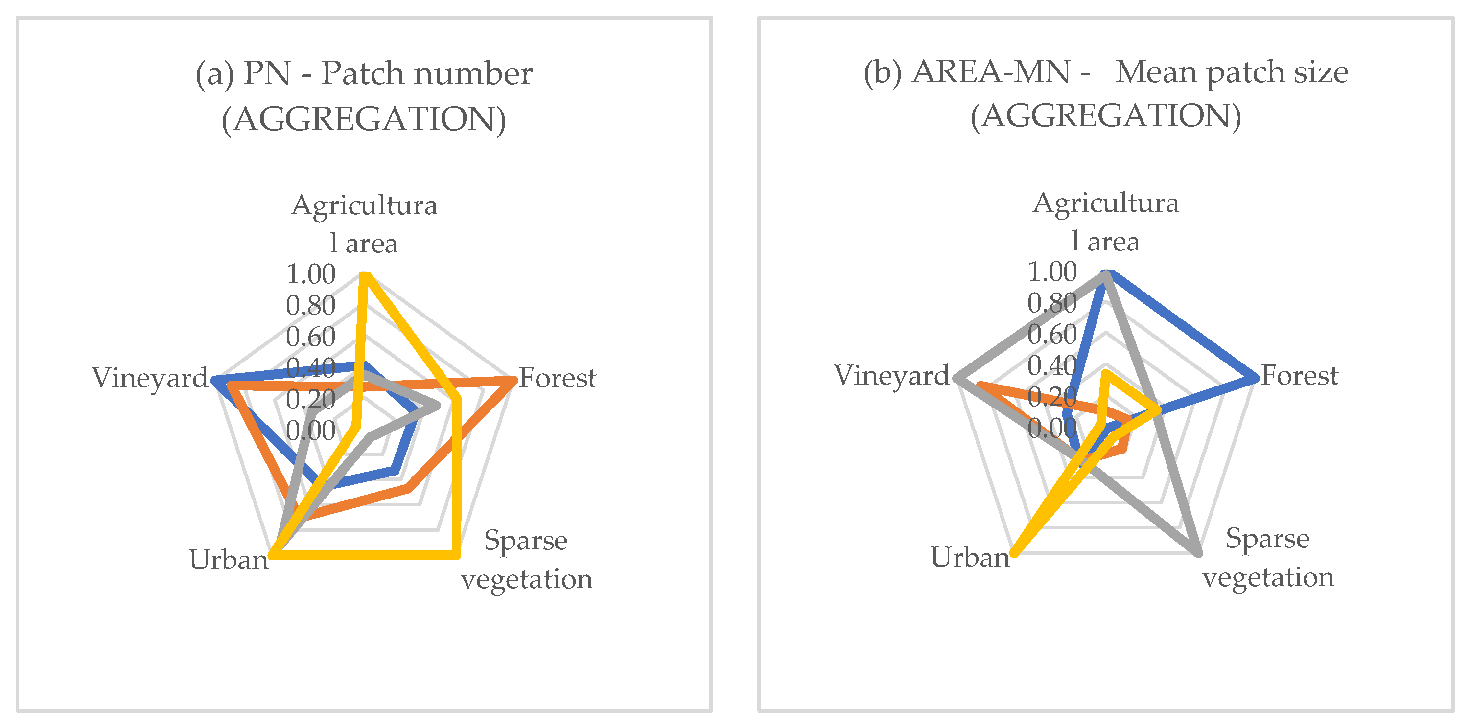
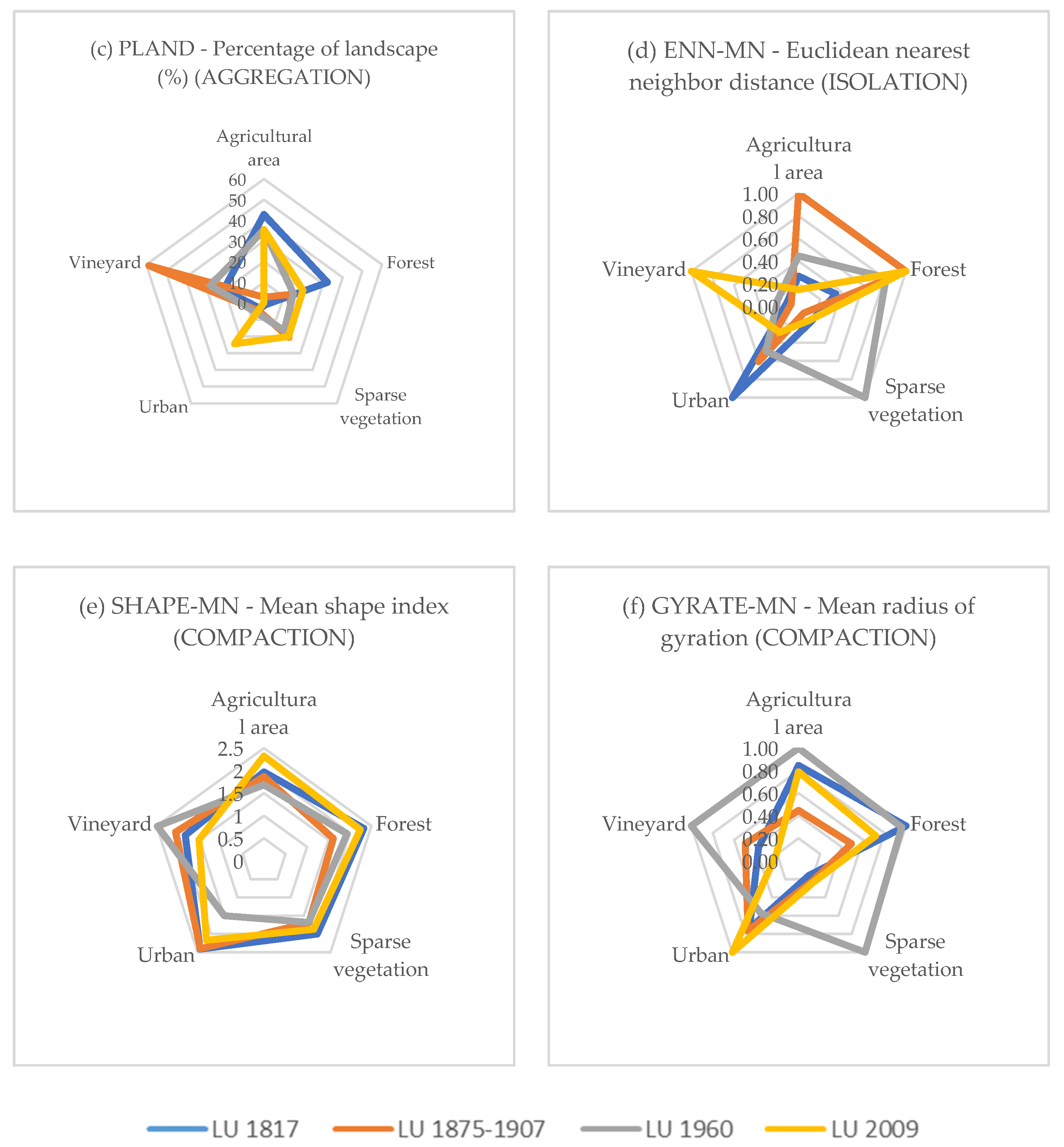
• Aggregation metrics. These metrics refer to the tendency of patch types to be spatially aggregated by means of the clustering of patches to form patches of a large size. This property is also usually used as an umbrella term to describe several closely related concepts of dispersion and interspersion, subdivision and isolation. Thanks to the aggregation process, it is usually possible to recognize the reduction in the number of total patches (PN metric, the simplest measure of subdivision; at the class level used to measure the fragmentation index), the increase of their mean areas (AREA_MN) and of their joint interpretation, i.e., the proportion of landscape occupied by the patch type (PLAND).
• Compaction metrics. These metrics mainly refer to landscape configuration, quantifying the geometric tendency of patches of the same type to assume a circular shape (the most compact). The inverse process is elongation. Among these metrics, the shape index (SHAPE_MN) measures the complexity of patch shape compared to a standard shape (square) of the same size. Further information is also obtained from metrics which analyse the composition of the landscape, such as the radius of gyration (GYRATE_MN). Specifically, this metric describes how far across the landscape a patch extends its reach. Thanks to the compaction process, it is possible to recognize a decrease in the SHAPE_MN metric and an increase in the GYRATE_MN one.
• Dispersion/isolation metrics. These metrics refer to the tendency of the distances between patches of the same type to increase. Dispersion metrics refer to the spatial distribution of a patch type (class). Euclidean nearest neighbour distance (ENN) is defined using simple Euclidean geometry as the shortest straight-line distance between the focal patch and its nearest neighbour of the same class, based on the mean distance between the two closest cell centres of the same type (ENN_MN). This metric measures the loss of structural connectivity without considering the characteristics of other land use/cover classes or the presence of barriers (and how they increase or decrease the cost of movement for different species). Thanks to the possible dispersion process, it is usually possible to recognize increases in ENN_MN. Specifically, for urban class type analysis, a greater isolation is considered as a sign of greater dispersion, i.e., a decreasing distance between urban patches is, in fact, an index of urban sprawl.

The four time steps of the LU/LC maps were processed not only in the study area but also for the whole perimeter of the thirteen municipalities belonging to the Park. To run Fragstat software [35,36], they were converted into raster images; the cell size was defined is 5 m × 5 m, i.e., less than one half of the lowest dimension of the smallest patch. Input grids were organized as square cells, referred to UTM WGS84 zone 33 N projection. Starting from the raster dataset of the LU/LC maps, the LMs were quantified, defining the role of the “8 cells neighbourhood” and the class metric as the sampling strategy.

2.4. Land Use Maps Comparison and Changes Detection

Successive paired thematic maps of land uses were compared using the open-source software Map Comparison Kit (MCK) [37], developed by the Research Institute for Knowledge Systems (RIKS) in Maastricht, the Netherlands. To run the comparison with the MCK software, it was necessary to apply subsequent geoprocessing and conversion tools. Firstly, to ensure that the spatial extension of all the maps was exactly the same, the intersect operation was needed, which allowed for the creation of a new boundary polygon common to all maps. The next step was the conversion of all the LU maps into TIFF raster images (rasterization), with a resolution of 20 m × 20 m. Finally, the raster files were transformed into raster-ASCII files to be imported into the MCK software [9].

The comparison between paired maps using MCK was based on the cell-by-cell method [36]. In order to implement this basic information on the similarities/differences in maps, the more flexible Kappa statistic indicator was used [37,38,39]. In fact, this statistic method is able to synthesize information on the position (such as spatial correlation) and quantity of cells divided by categories for a more balanced measure of similarity. In the present work, the Kappa algorithm, based on cell-by-cell comparison, was used. It expresses the degree of similarity between two categorical datasets. The Kappa statistic results from two types of similarity, similarity of quantity and similarity of location, according to the following Equation (1):

Kappa = K_Histo × K_Loc

(1)

where K_Histo stands for the assessment of the similarity in the position of the cell in two compared maps, whereas K_Loc provides an assessment of the quantity of similarity of the same two maps. Kappa, as well as K_Loc and K_Histo, is calculated on the basis of the contingency table [40], which details the cross-distribution of categories over the two maps according to the land-use change transition matrices. The table contains values that are expressed in hectares, and it is constructed according to a standard procedure:

• The rows report the land uses, expressed in hectares, of the first map;
• The columns report the land uses, expressed in hectares, of the first map.
• The diagonal of the table reports the hectares of each category that have not undergone any changes during the time step considered;

The last row and column provide the totals of the column and row. Each total row represents the total fraction of the areas of its category in the first map. Similarly, each total column represents the total fraction of the cells of the related category in the second map.

For the whole study area, the comparisons were performed on the following LU maps: LU 1817 and LU 1906; LU1906 and LU 1960; LU 1960 and LU 2009). The LU 1960–2009 and the LU 1817–LU 2009 comparisons were only processed within peri-urban areas.

3. Results

3.1. Land Use-Cover Maps Analysis and GIS Processing

The following intermediate outputs were further processed:

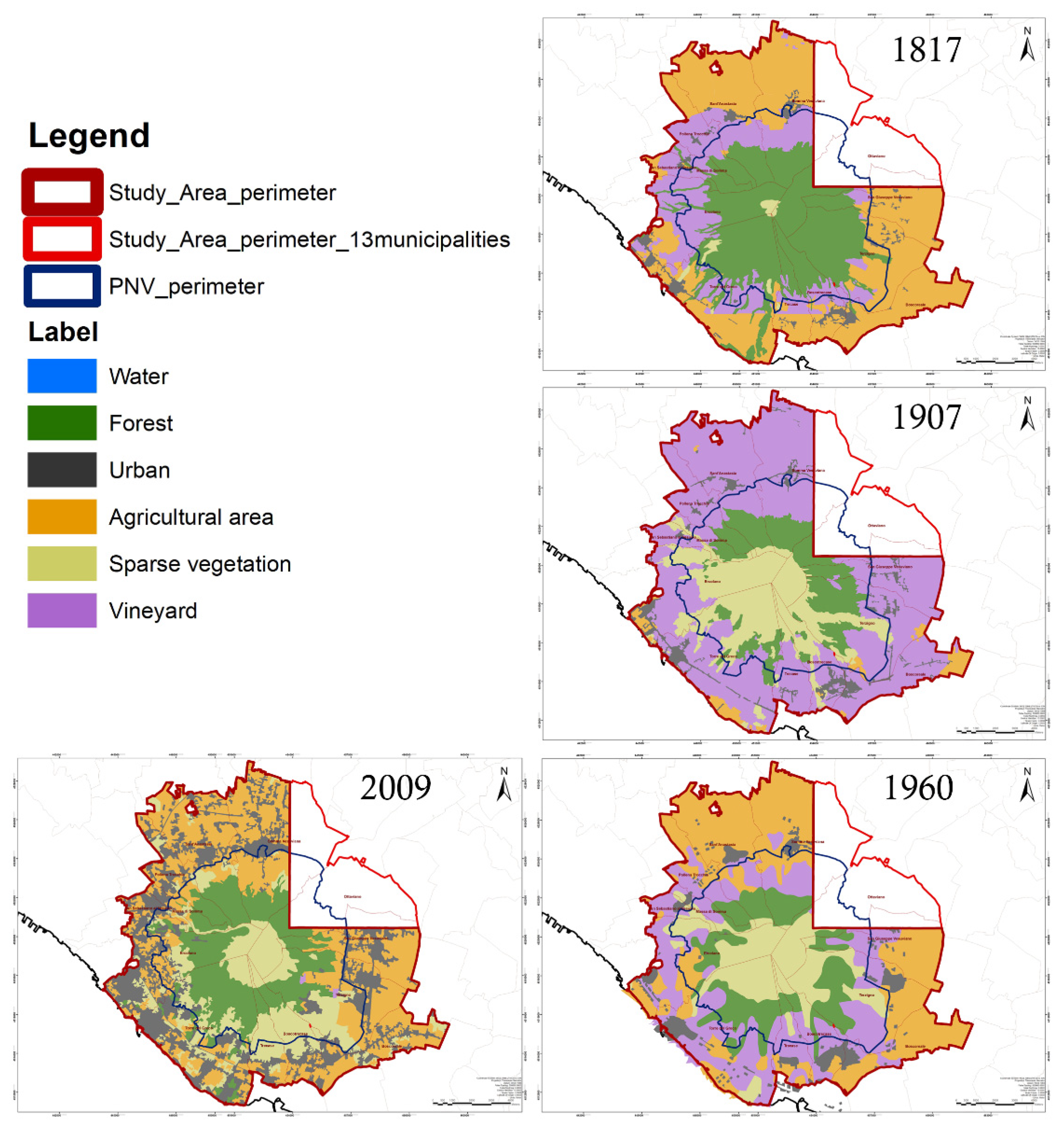
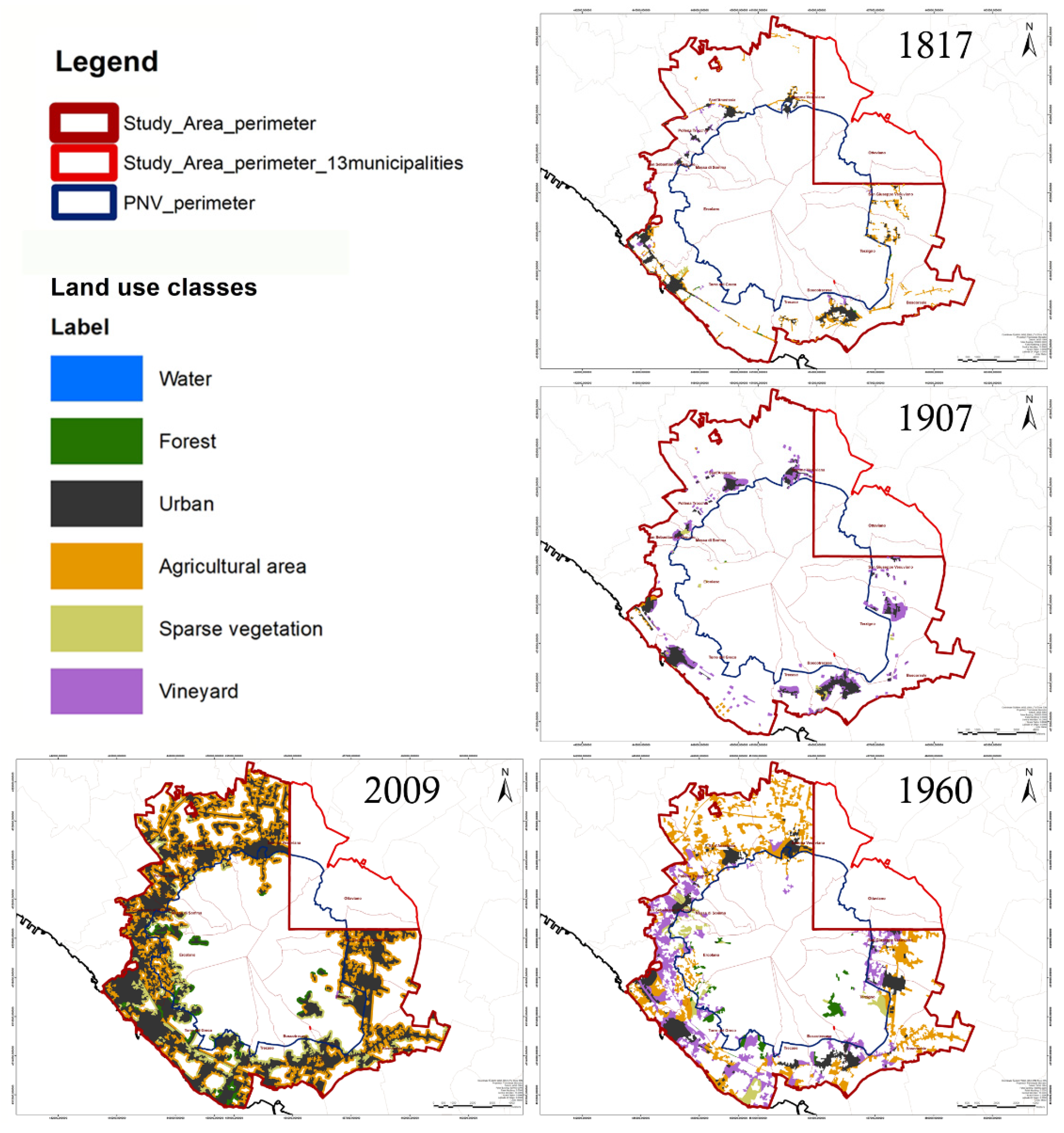
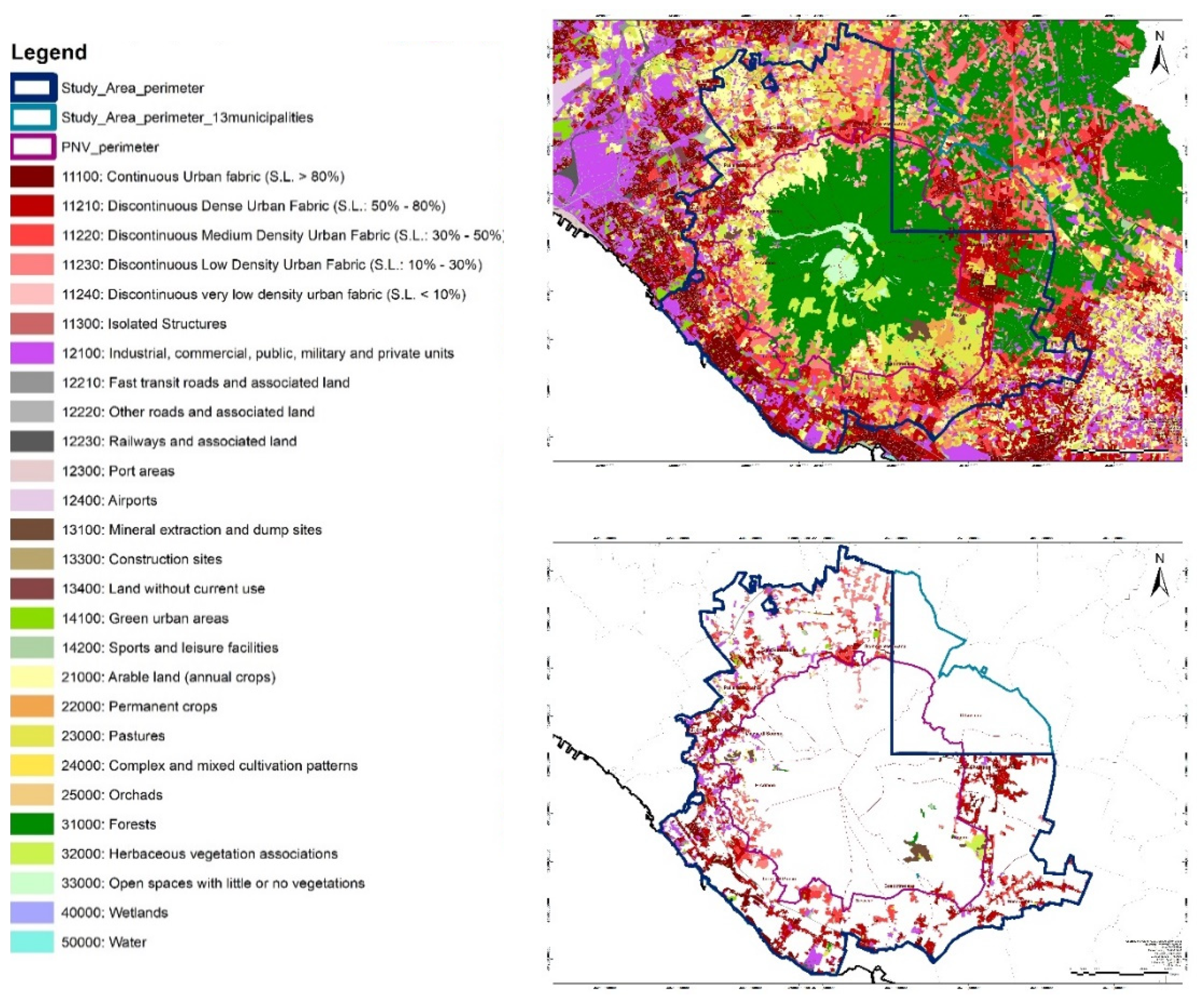
• Four LU maps of the whole study-area, with a common reclassified legend (Figure 5).
• Four LU maps, three of them devoted to each time step considered (1817, 1907, 1960) and clipped on the urban class recognizable in the subsequent time step (1907, 1960, 2009, respectively); a fourth land use map was clipped with the buffer areas of 100 m around the urban areas of the 2009 map (Figure 6).

All maps were georeferenced by means of a first order polynomial transformation and more than 100 points of correspondence for each one. The average RMS was between 20 m (1907 map) and 50 m (1817). The error associated with the transformation was calculated as the RMS sum of all the residuals of link points and showed a good assessment of the transformation’s accuracy [41]. Then, the MapAnalyst calculations, used for the assessment of visual accuracy, showed a root mean position error of between 14 and 18 m, highlighting the high accuracy level of the transformation process.

The resulting maps can be considered as intermediate outputs because they were the basis for subsequent analysis, both in terms of landscape configuration and composition, as well as LU structure changes.

Regarding the analysis of the whole study area, Figure 5 shows the distribution of the reclassified land uses in the four time steps. A greater compactness in the perimeters of the different types of land use in the maps of 1817, 1907 and 1960 can be observed (

Table 3. Percentage of land cover classes of the total study area for the different time steps.

Label	1817 % of the Total Area	1907 % of the Total Area	1960 % of the Total Area	2009 s % of the Total Area
Urban	3%	5%	6%	24%
Agricultural areas	43%	3%	36%	36%
Vineyard	21%	59%	27%	0%
Forest	32%	13%	15%	20%
Sparse vegetation	1%	21%	16%	20%
TOTAL	100%	100%	100%	100%

). On the other hand, the map of 2009 definitely presents a more articulated spatial configuration, both in terms of a greater detail of representation and in terms of the effect of urban expansion. Each map is significant for determining driving forces, pressures and trends with respect to each historical phase. Specifically:

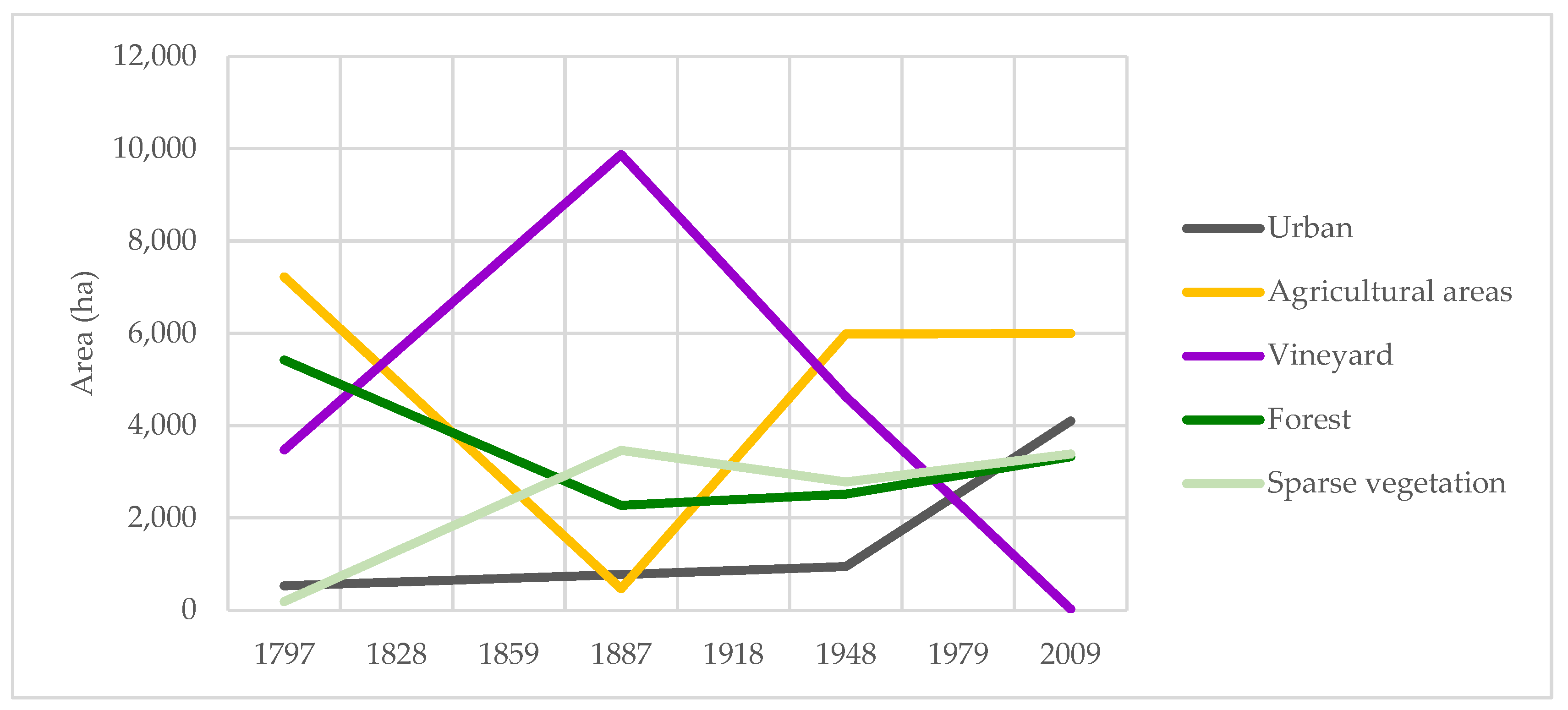
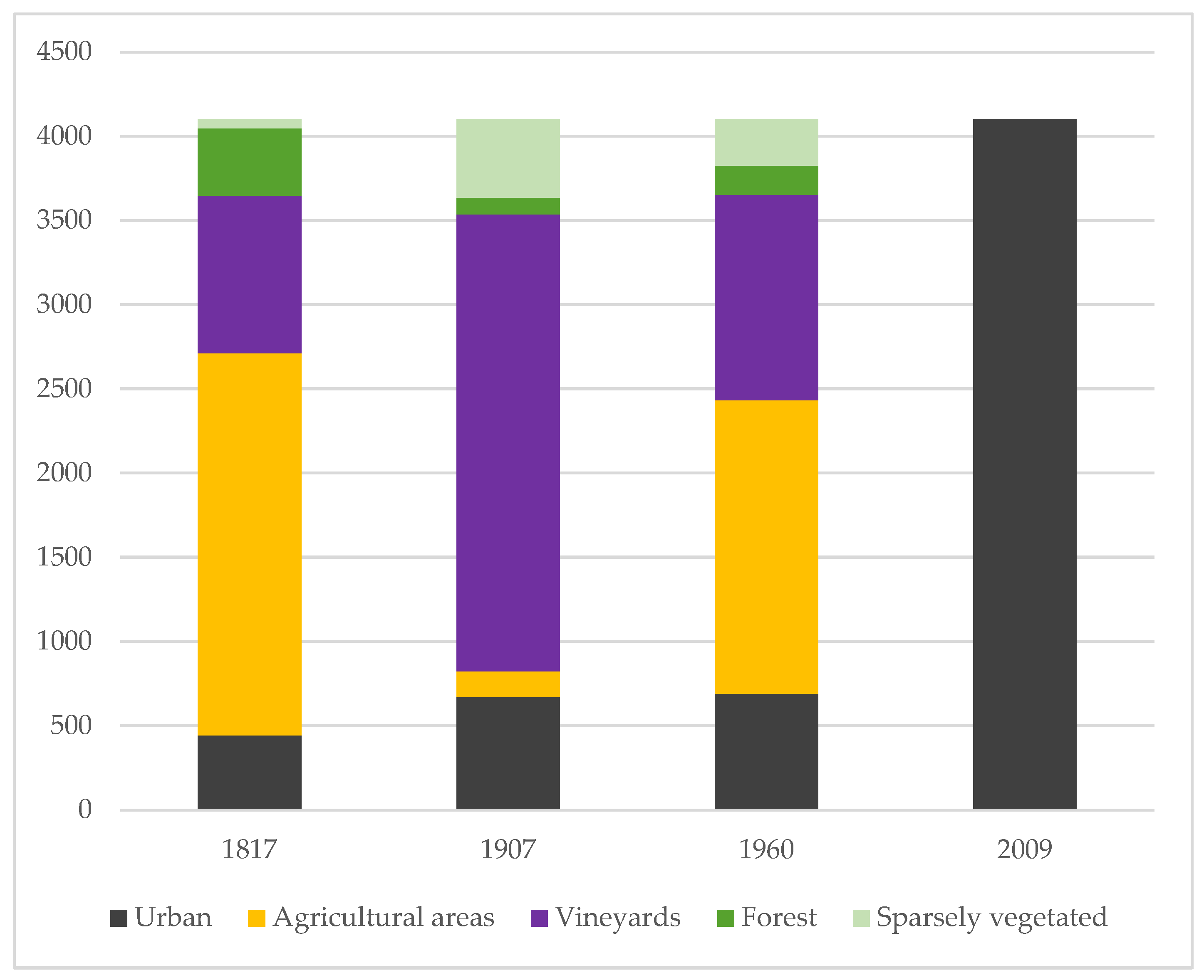
• the LU map of 1817 is characterized by the dominant presence of forests;
• the LU map of 1907 is characterized by the rapid and constant growth of vineyards and sparse vegetation;
• the LU map of 1960 is characterized by an initial reduction in vineyards;
• finally, the LU map of 2009, is characterized by significant anthropogenic pressure and urban sprawl and the almost total disappearance of vineyards.

Figure 7 shows the trend in the amount of areas expressed in ha with reference to each LU type for the whole period of the analysis (from 1817 to 2009). While almost all the LU classes show discontinuous trends over time, the urban class is the only one in constant growth, even when assuming an exponential growth rate since 1960.

Regarding LU trend analysis in urban/peri-urban areas (Figure 8), the comparison was performed by considering each time step map in relation to the year 2009 and each time step map in relation to the subsequent one.

The comparison of the LU map of 2009 with the 1817 one shows that urban expansion has principally affected agricultural areas (72% of which have disappeared, including vineyards in this class), but also a significant amount (10%) of forests have been lost. The comparison of the LU map of 2009 with the 1907 and 1960 ones shows a similar result, highlighting how, until 1960, the composition of the landscape was not subject to substantial variations in the study area. In fact, the strong transformation trend has taken place within the last five decades. The pairwise comparison of land use types, which referred to the urban perimeter of the subsequent period with for each time step (

Table 4. Time steps pairwise comparison in urban areas in terms of land use type.

	Land Uses in 1817 inside the Urban Areas of the 1907 Map		Land Uses in 1907 inside the Urban Areas of the 1960 Map		Land Uses in 1960 inside the Urban Areas of the 2009 Map
Label	ha	%	ha	%	ha	%
Urban	358	46%	401	42%	693	17%
Agricultural uses	331	43%	29	3%	1743	42%
Vineyards	56	7%	477	50%	1222	30%
Forest	10	1%	2	0%	169	4%
Sparse vegetation	17	2%	40	4%	277	7%
TOTAL	772	100%	949	100%	4104	100%

), shows similar trends. For both 1907 compared to 1817 and 1960 compared to 1907, the urban areas grown in agricultural ones (as sum of vineyards and other agricultural uses) represent 50% of new expansions. As seen above, very different conditions characterize the comparison between 2009 and 1960, in which new urban areas increased significantly to the detriment of agricultural areas. The new occupancy rate of the latter by urban sprawl in fact rose up to 70% and 80%, in other words, urban areas came to occupy soils which until that moment were still considered productive.

3.2. Landscape Metrics Analysis

Fragstat software was used for landscape metrics analysis. Fragstat results, in the form of a .csv file, were imported into Microsoft Excel and all values were normalized, except for PLAND, as reported in Figure 9. The results allow for the recognition of landscape development in terms of land composition and configuration.

In terms of the aggregation process, the patches number (PN) metric, which is the simplest measure of aggregation, shows a widespread increase for almost all the LU classes, especially for two time steps (1907 and 2009). Meanwhile, it is interesting to observe that in the 1960 time step, only the urban class grows. When compared with the mean patch size (AREA-MN), this metric also provides other useful information: as shown, in the 2009 time step, almost all the LU class types increase in number, but only the urban class also shows a significant increase in terms of mean size, in the same way that the vineyard class does in the 1907 time step. On the contrary, the 1960 time step is characterized by an increase in size of agricultural uses (both vineyards and other types) and sparse vegetation, as well as a decrease in the size of forest and urban patch types. The percentage of landscape (PLAND) metric, such as the PN one, is a fundamental measure for landscape compositions. The PLAND results show that agricultural uses have been a constant in the study area: by combining agricultural areas with vineyards, it was possible to appreciate their aggregation process, which began to decrease only in the last few decades, in favour of urban uses. These areas (the urban ones), only show an exponential increase in the last time step (2009).

In terms of the compaction process, the SHAPE metric highlights a general tendency to assume more irregular forms for patches of all types in the 2009 land use map. For the previous periods, the compactness of the forms of urban patches in 1960 was noted (probably always due to the lower resolution of the map), as was the compactness of the forms of forests in 1907 and agricultural areas in 1817. The GYRATE metric shows a compaction trend for the urban LU type during the two centuries of analysis. Forest and agricultural areas present, instead, the opposite process, with a reduction in the average amplitude of the radius of gyration. Furthermore, the 1960 map shows the maximum compaction of all the LU classes, except for the urban one, whereas the 1907 map shows lower values of compaction in all LU classes.

Finally, in terms of isolation or dispersion, the Euclidean nearest neighbour distance (ENN-MN) metric allows for the determination of the significant isolation of forests (due to their re-burning) and vineyards (do to their almost total disappearance) in the recent time step, with this taking place against the aggregation of the other LU classes, such as the urban type. It is interesting to observe how this situation is diametrically opposed to the one in 1817, in which urban areas were characterized by isolation, while others, especially agricultural areas and forests, had a strong character of aggregation.

3.3. Land Use Changes Comparison

The MCK software provided four contingency tables. These transformation matrices, reporting the number of cells, provide the cross distribution of the categories on the different pairwise maps.

As a first step, LU change analysis over the two hundred years, from 1817 to 2009, was performed. The main variations affect (

Table 5. Contingency table of land cover change for the period 1817–2009. Results represent the areas under change and are expressed in ha. Cells in orange report a loss in ha, while green ones report a net gain in ha.

LU_1817\LU_2009	1—Urban	2—Agricultural Uses	3—Vineyard	4—Forest	Sparse Vegetated	Sum LU_1817
1—Urban	7067.4	935.5	0.0	158.2	326.2	8487.3
2—Agricultural uses	36,290.1	67,409.9	0.0	789.9	11,028.4	115,518.2
3—Vineyard	14,938.6	21,299.6	0.0	3768.4	15,567.4	55,573.9
4—Forest	6386.2	6171.8	390.4	48,000.2	25,800.5	86,749.1
5—Sparse vegetated	898.5	73.9	0.0	468.8	1415.6	2856.7
Sum LU_2009	65,580.8	95,890.7	390.4	53,185.5	54,138.0

):

• urban areas, which have increased by almost 700% principally at the expense of agricultural areas, vineyards and, moderately, forests.
• sparse vegetation areas, which have increased up to 1800%, mainly producing a reduction in forests, but also in vineyards and agricultural areas.
• vineyards, which have experienced a decrease of 99%, nearly disappearing from the Vesuvius area; it is interesting to note that vineyards have completely disappeared the original areas of the 2009 LU map, while a few hectares were still detectable in areas occupied by forests in the past.

After partial time step analysis for the period of 1817–1907 (

Table 6. Contingency table of land cover change for the period 1817–1907. Results represent the areas under change and are expressed in ha. Cells in orange report a loss in ha, while green ones report a net gain in ha.

LU_1817\LU_1907	1—Urban	2—Agricultural Uses	3—Vineyard	4—Forest	5—Sparse Vegetated	Sum LU_1817
1—Urban	5724.5	343.2	2211.6	8.6	191.3	8479.2
2—Agricultural uses	5277.7	5552.0	100,559.2	578.0	3539.4	115,506.2
3—Vineyard	897.8	1024.5	42,826.9	2303.1	8504.8	55,557.0
4—Forest	165.7	528.6	11,800.7	33,074.6	41,172.0	86,741.6
5—Sparse vegetated	279.8	28.4	349.6	384.6	1930.1	2972.5
Sum LU_1907	12,345.4	7476.7	157,748.0	36,348.9	55,337.6

), we observed:

• a significant increase in sparse vegetation areas, over 1700%, almost exclusively at the expense of forest areas.
• a significant increase in vineyards, equal to nearly 200%, due to changes in land use from other categories of agricultural areas.

The first half of the twentieth century (1907–1960) allowed us to observe (

Table 7. Contingency table of land cover change for the period 1907–1960. Results represent the areas under change and are expressed in ha. Cells in orange report a loss in ha, while green ones report a net gain in ha.

LU_1907\LU_1960	1—Urban	2—Agricultural Uses	3—Vineyard	4—Forest	Sparse Vegetated	Sum LU_1907
1—Urban	6384.7	3758.5	2031.6	33.9	151.7	12,360.4
2—Agricultural uses	470.7	5358.0	1421.5	15.8	211.8	7477.8
3—Vineyard	7547.6	83,295.4	57,263.6	5801.2	3857.6	157,765.4
4—Forest	33.1	725.3	6276.0	21,928.1	7384.9	36,347.4
5—Sparse vegetated	639.0	2562.1	6978.3	12,427.6	32,823.0	55,430.0
Sum LU_1960	15,075.1	95,699.3	73,971.1	40,206.6	44,428.9

) a substantial return to agricultural activities (+1200%). All other land use classes show a partial conversion to agricultural uses, but vineyards were especially affected by these changes (−53%).

The last period examined, the second half of the Twentieth century, shows remarkably different developmental trends (

Table 8. Contingency table of land cover change for the period 1960–2009. Results represent the areas under change and are expressed in ha. Cells in orange report a loss in ha, while green ones report a net gain in ha.

LU_1960\LU_2009	1—Urban	2—Agricultural Uses	3—Vineyard	4—Forest	5—Sparse Vegetated	Sum LU_1960
1—Urban	11,053.0	2831.7	0.0	86.7	1112.9	15,084.3
2—Agricultural uses	27,890.1	59,665.6	0.0	970.2	7097.2	95,623.2
3—Vineyard	19,551.4	27,261.6	0.2	6541.6	20,581.0	73,935.9
4—Forest	2706.9	3521.2	184.2	25,634.7	8169.9	40,216.9
5—Sparse vegetated	4427.8	2633.3	206.0	19,949.4	17,175.4	44,391.8
Sum LU_2009	65,629.2	95,913.5	390.4	53,182.6	54,136.5

):

• the main variation concerns urban areas, which have increased by 330%, subtracting land from agricultural areas and vineyards.
• vineyards have almost completely disappeared (−99.5%); the few hectares still existing are obtained from areas previously affected by forests and sparse vegetation.

Regarding the Kappa statistics [42,43], it is possible to observe the following evidence (

Table 9. Kappa algorithms comparison.

	LU_1817\LU_1907	LU_1907\LU_1960	LU_1960\LU_2009	LU_1817\LU_2009
Kappa	0.18408	0.30037	0.27414	0.30206
KLocation	0.65165	0.55157	0.41714	0.63008
KHisto	0.28248	0.54457	0.65719	0.4794
Fraction correct	0.33094	0.45941	0.42165	0.46025

):

K values allow definition of a poor degree of LU class correspondence overall, which increases, moderately (discrete correspondence values), only in the pairwise comparison of 1907 with 1960.

• Higher K_Loc values in the nineteenth century (the comparison of the 1817 and 1907 maps) show that most categories are in identical positions in both maps.
• Higher K_Histo values in the last half century (the comparison of the 1960 and 2009 maps) show a fair permanence, with the amounts total hectares belonging to the various LU types remaining constant when not considering whether there has been a change in spatial location. This statistic is supported and confirmed by the data reported in Table 8, in which it is possible to recognize the lowest differences in area variation (with the exception of urban areas and vineyards, which offset each other) compared to the other periods considered.
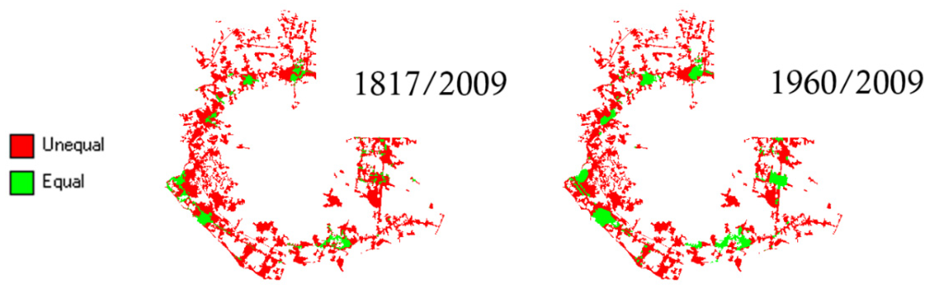
• The fraction correct statistic, which calculates the number of equal cells divided by the total number of cells, shows that the most significant land use transformations occurred between 1817 and 1907.

From the urban/peri-urban scale analysis, taking as its starting point the perimeter of urban areas in 2009, previous land uses in the same areas were determined. Specifically, the analysis referred to:

• a comparison between 2009 and 1960, in order to analyse the development of trends in the last fifty years;
• a comparison between 2009 and 1817, in order to analyse all of the changes affecting the land surrounding urban areas in the last two centuries.

The urban areas of the 2009 map cover 4102 ha, while these same areas were 530 ha in 1817 and 945 ha in 1960. The growth rate of urban areas between 1817 and 2009 is almost 800%. However, this change is distributed over the entire analysis period, which in this case is equal to about 200 years. The 1960 and 2009 comparison, in these terms, has a more significant impact: the growth rate of urban areas in this case is 500% but is spread over a much smaller number of years, about 60. The significant increase of the urban LU type over the last two centuries has inevitably affected other land use classes, as reported in

Table 10. Land uses in 1817 and 1960 maps, inside the perimeter of urban areas in the 2009 map (hectares).

Land Uses	Hectares 1817 Map	Hectares 1960 Map
1—Urban	7067.44	11,053
2—Agricultural uses	36,290.08	27,890.08
3—Vineyard	14,938.6	19,551.44
4—Forest	6386.16	2706.92
5—Sparse vegetated	898.52	4427.76
Sum Map	65,637.96	65,637.96

.

Specifically, the comparison between 1817 and 2009 highlights that more than 50% of current urban areas occupy lands which two centuries ago were destined for agricultural uses. This rises to almost 80% when vineyards are also considered. Of the increase in urban areas, 10% were previously forest areas.

In addition, in the case of the comparison between 1960 and 2009, the urban areas that increased were previously agricultural areas, both vineyards and other types. The urbanization process scarcely affected forests, while it occupied 7% of sparsely vegetated areas, probably due to their increase in surface, in the 1960 map, related to the volcanic eruption of 1944. The Kappa statistics are not noteworthy at a local-urban scale, because the comparisons were made with a 2009 map which present only one class; thus, the statistics are distorted and take values of either 0 or 1.

Figure 10 spatially illustrates the areas in which the urban use type is the same (in green) and the areas in which land use changes occurred (in red).

4. Discussion

The developed analyses, focused on land use in the Vesuvius area over the last two centuries, have made it possible to recognize trends in LUCC using a qualitative–quantitative approach.

The historical cartography available for the study area exhibited a high degree of reliability and the transformations they showed were connected to different anthropogenic and natural driving forces which intertwine and alternate. The graphic land representation/simulation and the process of interpreting the historical cartography effectively supported the comparative diachronic reading of the structure of the landscape in terms of its typological characteristics and invariants.

A first aspect to consider concerns the level of detail on the maps: the resolution of the historical maps (between 1:25,000 and 1:50,000) made almost all of them substantially comparable. The only exception was the 1960 map, whose resolution (1:200,000) made it useful in comparison with other maps in terms of the qualitative definition of land use change trends and in the overall quantification of area amounts, but less significant in terms of landscape metrics, especially for issues related to land configuration.

Accuracy is another interesting aspect to consider in relation to the use of historical maps. In the present work, a high level of accuracy was demonstrated by the low values of RMS error in ESRI ArcMAP and the MPE and SD indicators in the MapAnalyst software.

When it comes observed transformations, overall, the reference period (1817–2009) records a reduction in forest and agricultural areas, to the benefit of urban and sparse vegetation ones:

• the forests that used to make up 32% of the territory currently occupy 20% of it;
• agricultural areas and vineyards previously made up 43% and 21% of the territory, respectively, whereas now they make up 36% of it;
• sparse vegetation areas went from 1% to 20% in 2009;
• urban areas increased from 3% to 24%.

The driving forces behind these changes are closely intertwined. Forest reduction, for example, must be read in the context of increases in both scattered vegetation areas and urban areas and the replacement of soils with agricultural areas.

Almost 30% of the forests of 1817 are today covered by scattered vegetation areas. This ratio rises to 47% in 1907 compared to the 1817 map and stabilizes at 20% in the following two periods. In forestation terms, the last fifty years show a reversal of this trend when compared to the beginning of the century.

The particular “nature” of the national park, with the presence of a volcano, explains the amount of variation (increases and decreases in scattered vegetation areas, which often replace forests) in areas close to the cone. It is possible that, due to the effect of the cessation of Vesuvius activity (the last eruption was in 1944), as well as the effect of the establishment of the natural protected area in 1991 (along with consequent policies of nature protection), in the recent decades, a re-forestation process has taken place near the crater.

Analysis of the replacement of the original (1817) 400 ha of forests with anthropic areas (2009), in the different temporal phases, highlights a process which has unfolded over two centuries. The greatest impact on forests has occurred in the last fifty years, but, in the same period, this aggression has been balanced out by new reforestation in areas previously affected by vineyards and sparse vegetation. Instead, in the previous period (from 1960 to 1817), the process of urban growth had mainly affected agricultural areas and vineyards.

The dynamic of the “urban” LU type, in terms of the overall area amount during the two centuries analysed, shows an increase trend. The comparison of this trend with that of the population (Figure 2) allows for the observation that the growth rate was quite different: urban areas in fact went from 590 ha to 4102 ha, with an increase of 700%, while the population went from 65,000 to 312,000 inhabitants, with a growth rate of 400%. Detailed analysis by historical period (time steps) also highlights that the most substantial population increase in the study area occurred in the first half of the twentieth century (between 1911 and 1961), while the most significant rate of urban expansion during the second half of the twentieth century, between 1960 and 2009. It can be deduced that the increase in the “urban” LU type can be considered to be only partially linked to the population. The consumption (and consequent waterproofing) of soil was certainly conditioned by the spread of new models of urban and infrastructural expansion in the territory as an effect of the Italian economic boom after the Second World War.

Anthropic pressure, and the economic activities associated with it, on the one hand help to shape and characterize the area, but on the other hand they also compromise delicate ecological and environmental balances. In this specific context, the expansion of urban areas has had a significant impact on agricultural and natural soils. Such conditions have certainly also influenced those essential “services” generally provided by natural capital, i.e., the ecosystem services, such as air quality, natural filtration, land conservation, erosion regulation, genetic diversity typical of areas with extensive agriculture, habitat quality and so on. These aspects, strictly connected to LUC studies, may be the subject of further investigation in the near future in order to check trends in the use and protection of ecosystem services and to quantify the current services provided by existing natural capital based on LUC scenarios. All these aspects can be used support the activities of decision-makers, sensitizing administrations and populations towards not only socio-economic development, but also environmental issues. A further aspect that has not been explored here, for reasons of level of detail, but which should be further investigated, is the definition of an objective method for the determination of the urban perimeter, for the purpose then classifying the remaining part of the territory as non- urban. In the last few centuries, the urban perimeter has certainly been better defined, as also underlined by the metrics on the shape. Starting from the 1960s, on the other hand, it became necessary to classify both continuous and discontinuous urban areas. Today, we could talk of different forms of discontinuous urban areas that become new categories and new classes of land uses and coverings.

In the present paper, from a physical/spatial point of view, the landscape metrics highlights the consolidation of a new model of urban expansion (in its structure, composition and configuration). Specifically, the used metrics show the growing tendency towards the aggregation for only of the “urban uses” class. The connective net, the inter-space between one urban settlement and another, has been progressively absorbed by anthropic settlements. Urban areas, particularly in the last half century, are the only land use class that has seen greater compactness, even in the face of the greater articulation of the perimeters. Specific investigations, at a greater level of detail, will have to be carried out in future work to investigate the possible connections between the composition and configuration of the landscape and the socio-economic characteristics of areas of urban expansion.

From a functional point of view, in order to investigate whether this process is characterized as “integration” or rather simple “aggregation”, the previous results were compared with a further database: the URBAN ATLAS map (2018) of the Naples province. This document classifies the land covers with a particular level detail for anthropized areas. Unlike the Corine Land Cover inventory, which in the 2018 version deepens the fourth level classification for “natural and semi-natural areas”, the Urban Atlas of the province of Naples describes urban and anthropic areas up to the fourth level.

Figure 11 and

Table 11. Urban Atlas (2018) land uses in urban expansion areas between 1960–2009.

Code	Item 2018	Area (ha)	%
11210	Discontinuous dense urban fabric (S.L.: 50–80%)	1082.0	31.7%
11220	Discontinuous medium density urban fabric (S.L.: 30–50%)	561.2	16.5%
12100	Industrial, commercial, public, military and private units	360.5	10.6%
11230	Discontinuous low density urban fabric (S.L.: 10–30%)	340.9	10.0%
11100	Continuous urban fabric (S.L.: >80%)	298.3	8.8%
12220	Other roads and associated land	254.6	7.5%
13100	Mineral extraction and dump sites	85.2	2.5%
23000	Pastures	78.8	2.3%
21000	Arable land (annual crops)	60.5	1.8%
32000	Herbaceous vegetation associations (natural grassland, moors)	45.3	1.3%
14100	Green urban areas	42.6	1.3%
14200	Sports and leisure facilities	40.5	1.2%
12230	Railways and associated land	35.5	1.0%
12210	Fast transit roads and associated land	34.7	1.0%
31000	Forests	31.9	0.9%
11240	Discontinuous very low density urban fabric (S.L.: < 10%)	25.0	0.7%
13400	Land without current use	15.1	0.4%
50000	Water	6.7	0.2%
22000	Permanent crops (vineyards, fruit trees, olive groves)	5.4	0.2%
11300	Isolated structures	2.8	0.1%
13300	Construction sites	1.4	0.0%
	TOTAL	3408.8	100.0%

show the spatial articulation of new urban expansions by means of Urban Atlas map. The last urban growth (1960–2009) entails almost 3500 ha and almost 50% of this consists of “discontinuous urban fabric” with medium and dense densities. This percentage rises to 85% when also taking into account the low-density “urban discontinuous” typology, industrial and commercial areas, extraction sites and roads. The only land composition analysis avoiding the issues of environmental and social quality concerning these transformations (issues that will be the subject of future work) shows an urbanization process which has led to the saturation of the territory and the waterproofing of previous agricultural soils. There is the almost total absence of soils destined for public services, such as urban green areas and areas for sport and recreation, although this was foreseen by national urban planning law (of 1942) and urbanistic standards national legislation (1968). It should be further highlighted that within the new urban expansion, about 15 ha (0.5%) is classified as areas without use or abandoned.

This study shows that, historically, urban expansion in the Vesuvius area has mainly occurred at the expense of agricultural areas. The awareness of this must focus the attention of planners and political decision-makers with respect to current suburbs: 95% of the urban buffer areas consist of agricultural land. To avoid new land use changes characterized by strong waterproofing and low social and environmental quality standards, it will be appropriate to adopt new measures and strategies for the protection of agricultural heritage. Specific investigations undertaken at a greater level of detail will have to be carried out in future work to investigate the possible connections between the composition and configuration of the landscape and the socio-economic characteristics of areas of urban expansion.

The present work, which developed a methodology that analyses historical LUCC in the Vesuvius area in terms of landscape metrics, may support local administrators in their attempts to implement possible strategies to mitigate the effects of the rapid urban development. The study contributes to the urban/peri-urban debate, focusing on the use of different methods which can help to highlight the interactions between the physical, functional and visual components of the landscape. The integrated land-use and landscape planning methods belong to a holistic approach which encompasses the definition of driving forces, multi-criteria assessments, spatial modelling, an impact assessment by means of ecosystems services and landscape metrics approaches, and the support of GIS techniques. All of these methods, together with the creation of increasingly articulated and shared databases (also based on historical sources and database), could become important and strategic measures when it comes to supporting decision-makers and for sharing and transferring information with stakeholders.

5. Conclusions

The interdependence between urban and non-urban landscapes, which has been stratified over the centuries, has created a complex network of physical, functional and perceptual connections, which need to be taken into account in the processes of landscape governance. The relationship between anthropic and natural and between urban areas and non-urban landscapes, today characterizes a complex bio-cultural system, which requires a unitary approach which can be successfully implemented by an accurate multi-temporal analysis of the relationships between constituent parts.

The paper intends to contribute to land management by starting from historical analyses, not only for the purpose of increasing knowledge of the current state of the landscape, but also in terms of support when it comes to mitigating or limiting the degradation of phenomena (starting from the recognition of the causes) as well as the enhancement of their potential (working on the valuable elements that still exist). Decisions involving environmental characteristics and issues essentially depend on the landscape and how it evolves in space and in time. In these terms, the developed approach intends to support land-use planning and management with specific attention paid to extra-urban areas: these areas are particularly fragile and vulnerable as they still have a high potential for transformability. The method presents an approach for gaining knowledge about the landscape, the results of which, once shared with stakeholders an decision-makers, will contribute to building a transparent planning process.

Data on land-cover/land-uses and their changes over the last two centuries can constitute important information for decision makers, both as a basis for the implementation of sustainable management strategies for the territory, and as reference in the assessment and monitoring of the effectiveness of policies implemented in the past in terms of environmental and socio-economic (as well as agricultural) activities.

This work aims to contribute to landscape governance, taking as its starting point the correlation between intrinsic landscape characteristics and quantitative indices expressed by the territory according to a space-time approach. The paper intends to support a new approach to the urban–rural dialectic, with a view towards integration rather than opposition. Peripheral areas, peri-urban areas, new types of territories and interface areas, are today often characterized by fragmentation. A specific study of these areas can contribute to a new approach, considering them to be an opportunity rather then a problem, as a place of recomposition in which green infrastructures, ecosystem services also aimed at the urban environment, such as peri-urban forestry, agricultural parks, road networks for “soft mobility” and social gardens, play an important role. These contexts can become the pivot for a new territorial re-birth and re-development which is open to urban as well as non-urban landscapes and which also supports telematics and road networks.

References

- Salvati, L. Agro-forest landscape and the ‘fringe’ city: A multivariate assessment of land-use changes in a sprawling region and implications for planning. Sci. Total Environ. 2014, 490, 715–723. [Google Scholar] [CrossRef] [PubMed]
- Terbeck, F.J. Defining Suburbs: An Evaluation and Comparison of Four Methods. Prof. Geogr. 2020, 72, 586–597. [Google Scholar] [CrossRef]
- Simon, D. Urban environments: Issues on the peri-urban fringe. Ann. Rev. Env. Resour. 2008, 33, 167–185. [Google Scholar] [CrossRef]
- Agarwal, C. A Review and Assessment of Land-Use Change Models: Dynamics of Space, Time, and Human Choice; UFS Technical Report NE-297; U.S. Department of Agriculture Forest Service, Northeastern Forest Research Station: Burlington, VT, USA, 2002. Available online: http://www.fs.fed.us/ne/newtown_square/publications/technical_reports/pdfs/2002/gtrne297.pdf (accessed on 10 May 2021).
- Murray-Rust, D.; Robinson, D.T.; Guillem, E.; Karali, E.; Rounsevell, M. An open framework for agent based modelling of agricultural land use change. Environ. Model. Softw. 2014, 61, 19–38. [Google Scholar] [CrossRef]
- Zhang, L.; Nan, Z.; Yu, W.; Ge, Y. Modeling Land-Use and Land-Cover Change and Hydrological Responses under Consistent Climate Change Scenarios in the Heihe River Basin, China. Water Resour. Manag. 2015, 29, 4701–4717. [Google Scholar] [CrossRef]
- Pindozzi, S.; Cervelli, E.; Recchi, P.F.; Capolupo, A.; Boccia, L. Predicting land use change on a broad area: Dyna-CLUE model application to the Litorale Domizio-Agro Aversano (Campania, South Italy). J. Agric. Eng. 2017, 48, 27. [Google Scholar] [CrossRef]
- Cervelli, E.; di Perta, E.S.; Pindozzi, S. Energy crops in marginal areas: Scenario-based assessment through ecosystem services, as support to sustainable development. Ecol. Indic. 2020, 113, 106180. [Google Scholar] [CrossRef]
- Pindozzi, S.; Cervelli, E.; Capolupo, A.; Okello, C.; Boccia, L. Using historical maps to analyze two hundred years of land cover changes: Case study of Sorrento peninsula (south Italy). Cartogr. Geogr. Inf. Sci. 2015, 43, 250–265. [Google Scholar] [CrossRef]
- Uuemaa, E.; Antrop, M.; Roosaare, J.; Marja, R.; Mander, U. Landscape Metrics and Indices: An Overview of Their Use in Landscape Research. Liv. Rev. Landsc. Res. 2009, 3, 1–28. [Google Scholar] [CrossRef]
- Frank, S.; Fürst, C.; Koschke, L.; Makeschin, F. A contribution towards a transfer of the ecosystem service concept to land-scape planning using landscape metrics. Ecol. Indic. 2012, 21, 30–38. [Google Scholar] [CrossRef]
- Gustafson, E.J. Minireview: Quantifying Landscape Spatial Pattern: What Is the State of the Art? Ecosystems 1998, 1, 143–156. [Google Scholar] [CrossRef]
- McGarigal, K. Landscape pattern metrics. In Encyclopedia of Environmetrics; El-Shaarawi, A.H., Piegorsch, W.W., Eds.; John Wiley & Sons: Chichester, UK, 2002; pp. 1135–1142. [Google Scholar]
- McGarigal, K. Fragstats Help. Amherst: Department of Environmental Conservation University of Massachusetts. 2015. Available online: https://www.umass.edu/landeco/research/fragstats/documents/fragstats.help.4.2.pdf (accessed on 10 May 2021).
- Geoghegan, J.; Wainger, L.; Bockstael, N.E. Spatial landscape indices in a hedonic framework: An ecological economics analysis using GIS. Ecol. Econ. 1997, 23, 251–264. [Google Scholar] [CrossRef]
- Alberti, M.; Marzluff, J.M. Ecological resilience in urban ecosystems: Linking urban patterns to human and ecological functions. Urban. Ecosyst. 2004, 7, 241–265. [Google Scholar] [CrossRef]
- Liu, M.; Hu, Y.-M.; Li, C. Landscape metrics for three-dimensional urban building pattern recognition. Appl. Geogr. 2017, 87, 66–72. [Google Scholar] [CrossRef]
- Madanian, M.; Soffianian, A.R.; Koupai, S.S.; Pourmanafi, S.; Momeni, M. Analyzing the effects of urban expansion on land surface temperature patterns by landscape metrics: A case study of Isfahan city, Iran. Environ. Monit. Assess. 2018, 190, 189. [Google Scholar] [CrossRef]
- Cervelli, E.; Scotto Di Perta, E.; Di Martino, A.; Faugno, S.; Pindozzi, S. Historical land use change and landscape pattern evolution study. In Environmental and Territorial Modelling for Planning and Design; Smart City, Urban Planning for a Sustainable Future; Leone, A., Gargiulo, C., Eds.; FedOAPress: Napoli, Italy, 2018; Volume 4, pp. 189–197. [Google Scholar]
- Vesuvian Observatory. The Eruptions from 1631 to 1944. Available online: www.ov.ingv.it/ov/it/catalogo-1631-1944.html (accessed on 12 July 2021).
- Vianello, G.; Antisari, L.V. Pedo-environmental evolution and agricultural landscape transformation. Ital. J. Agron. 2009, 4, 5–12. [Google Scholar] [CrossRef] [Green Version]
- Pelorosso, R.; Leone, A.; Boccia, L. Land cover and land use change in the Italian central Apennines: A comparison of as-sessment methods. Appl. Geogr. 2009, 29, 35–48. [Google Scholar] [CrossRef]
- Brovelli, M.A.; Minghini, M. Georeferencing old maps: A polynomial-based approach for Como historical cadastres. e-Perimetron 2012, 7, 97–110. [Google Scholar]
- Mori, A. Le Carte Geografiche. Costruzione Interpretazione e Applicazioni Pratiche [The Maps. Construction Inter-Pretation and Practical Applications]; Libreria Goliardica: Pisa, Italy, 1989. (In Italian) [Google Scholar]
- Petit, C.; Scudder, T.; Lambin, E. Quantifying processes of land-cover change by remote sensing: Resettlement and rapid land-cover changes in south-eastern Zambia. Int. J. Remote Sens. 2001, 22, 3435–3456. [Google Scholar] [CrossRef]
- Rhemtulla, J.M.; Mladenoff, D.J.; Clayton, M.K. Regional land-cover conversion in the U.S. upper Midwest: Magnitude of change and limited recovery (1850–1935–1993). Landsc. Ecol. 2007, 22, 57–75. [Google Scholar] [CrossRef]
- Wan, L.; Zhang, Y.; Zhang, X.; Qi, S.; Na, X. Comparison of land use/land cover change and landscape patterns in Honghe National Nature Reserve and the surrounding Jiansanjiang Region, China. Ecol. Indic. 2015, 51, 205–214. [Google Scholar] [CrossRef]
- Ferreira, H.; Botequilha-Leitão, A. Integrating landscape and water resources planning with focus on sustainability. In From Landscape Research to Landscape Planning. Aspects of Integration, Education and Application; Tress, B., Tress, G., Fry, G., Opdam, P., Eds.; Springer: Dordrecht, The Netherlands, 2005; pp. 143–159. [Google Scholar]
- Frank, S.; Fürst, C.; Lorz, C.; Koschke, L.; Abiy, M.; Makeschin, F. Chances and limits of using landscape metrics within the interactive planning tool “Pimp Your Landscape”. In Proceedings of the Land Mod 2010, Montpellier, France, 3–10 February 2010; p. 13. [Google Scholar]
- Uuemaa, E.; Mander, Ü.; Marja, R. Trends in the use of landscape spatial metrics as landscape indicators: A review. Ecol. Indic. 2013, 28, 100–106. [Google Scholar] [CrossRef]
- Dematteis, G. Suburbanización y periurbanización. Ciudades anglosajonas y ciudades Latinas, English cities and Latin cit-ies. In La Ciudad Dispersa. Suburbanización y Periferias, The Dispersed City. Suburbanization and Outlying Areas; Monclús, J., Ed.; Centre de Cultura Contemporánea de Barcelona: Barcelona, Spain, 1998; pp. 17–33. [Google Scholar]
- Franco, D.; Bombonato, A.; Mannino, I.; Ghetti, P.; Zanetto, G. The evaluation of a planning tool through the landscape ecology concepts and methods. Manag. Environ. Qual. Int. J. 2005, 16, 55–70. [Google Scholar] [CrossRef] [Green Version]
- Dematteis, G.; Governa, F. Urban form and governance: The new multi-centred urban patterns. In Change and Stability in Urban Europe; Andersson, H., Jorgensen, G., Joye, D., Ostendorf, O., Eds.; Routledge: London, UK, 2017; pp. 27–44. [Google Scholar]
- Aguilera-Benavente, F.; Valenzuela, L.M.; Botequilha-Leitao, A. Landscape metrics in the analysis of urban land use patterns: A case study in a Spanish metropolitan area. Landsc. Urban Plan. 2011, 99, 226–238. [Google Scholar] [CrossRef]
- Nong, D.H.; Lepczyk, C.A.; Miura, T.; Fox, J.M. Quantifying urban growth patterns in Hanoi using landscape expansion modes and time series spatial metrics. PLoS ONE 2018, 13, e0196940. [Google Scholar] [CrossRef] [Green Version]
- McGarigal, K.; Cushman, S.A.; Ene, E. FRAGSTATS v4: Spatial Pattern Analysis Program for Categorical and Continuous Maps. University of Massachusetts, Amherst. Computer Software Program Produced by the Authors at the University of Massachusetts. 2012. Available online: https://www.umass.edu/landeco/research/fragstats/fragstats.html (accessed on 15 July 2021).
- Map Comparison Kit Software. Available online: http://mck.riks.nl/ (accessed on 10 May 2021).
- Visser, H.; De Nijs, T. The map comparison kit. Environ. Modell. Softw. 2006, 21, 346–358. [Google Scholar] [CrossRef]
- Pontius, R.G., Jr. Comparison of categorical maps. Photogr. Eng. Rem. S 2000, 66, 1011–1016. [Google Scholar]
- Hagen, A. Multi-Method Assessment of Map Similarity. In Proceedings of the Fifth AGILE Conference on Geographic Information Science, Palma, Spain, 25–27 April 2002; pp. 171–182. [Google Scholar]
- Available online: http//:www.esri.com (accessed on 12 July 2021).
- Pontius, R.G., Jr.; Millones, M. Death to Kappa: Birth of quantity disagreement and allocation disagreement for accuracy assessment. Int. J. Remote Sens. 2011, 32, 4407–4429. [Google Scholar] [CrossRef]
- Sadeghbeygi, A.; Moravej, K.; Delavar, M.A. Replacing kappa index with quantitative and spatial agreement and disa-greement components for the accuracy assessment of different thematic maps. Sci. Res. Quart. Geogr. Data 2021, 29, 77–87. [Google Scholar]