Article

Learning Human Strategies for Tuning Cavity Filters with Continuous Reinforcement Learning

1
Shenzhen Institute of Advanced Technology, Chinese Academy of Sciences, Shenzhen 518055, China
2
Guangdong Provincial Key Laboratory of Robotics and Intelligent System, Shenzhen Institute of Advanced Technology, Chinese Academy of Sciences, Shenzhen 518055, China
3
Guangdong-Hong Kong-Macao Joint Laboratory of Human-Machine Intelligence-Synergy Systems (2019B121205007), Shenzhen Institute of Advanced Technology, Chinese Academy of Sciences, Shenzhen 518055, China
*
Author to whom correspondence should be addressed.
Appl. Sci. 2022, 12(5), 2409; https://doi.org/10.3390/app12052409
Submission received: 12 January 2022 / Revised: 10 February 2022 / Accepted: 21 February 2022 / Published: 25 February 2022
(This article belongs to the Special Issue New Trends in the Control of Robots and Mechatronic Systems)

Abstract

:
Learning to master human intentions and behave more humanlike is an ultimate goal for autonomous agents. To achieve that, higher requirements for intelligence are imposed. In this work, we make an effort to study the autonomous learning mechanism to solve complicated human tasks. The tuning task of cavity filters is studied, which is a common task in the communication industry. It is not only time-consuming, but also depends on the knowledge of tuning technicians. We propose an automatic tuning framework for cavity filters based on Deep Deterministic Policy Gradient and design appropriate reward functions to accelerate training. Simulation experiments are carried out to verify the applicability of the algorithm. This method can not only automatically tune the detuned filter from random starting position to meet the design requirements under certain circumstances, but also realize the transfer of learning skills to new situations, to a certain extent.

1. Introduction

As dominators of the earth, human beings have higher intelligence than any other biological species. Humans are skilled in summarizing rules from observed phenomena, forming knowledge, and applying it to understanding new things. Throughout history, the evolution of humans is basically the process by which new methods and techniques are created to alleviate human labor, thus promoting the development of science and technology. As one of the greatest inventions in the 20th century, robotics has made great progress since the late 1950s. The emergence of robots is the inevitable trend of social and economic development, and its rapid growth has been improving the level of social production and the quality of human life.
Although people are eager to have robots in their homes, there is no doubt that the impact of robots on manufacturing is even greater, especially in the last decade when traditional manufacturing has undergone unprecedented changes. Due to the yearning for a better life, many people are unwilling to choose dangerous or boring jobs, which makes different types of human jobs face labor shortages. In this context, industrial robots show extraordinary ability in replacing human labor and improving productivity. However, some tasks that rely heavily on human dexterity or intelligence remain difficult to replace by robots. On one hand, while most industrial robots are adept at repetitive tasks, they are not flexible enough to manipulate forces, especially for some precision or fine machining; on the other hand, most robots today and fully automated production lines are not very good at understanding human intentions or learning sequential strategies from human behavior. Therefore, these automated devices are very sensitive to changes in context. To solve these problems, intelligent learning algorithms and human demonstrations aimed at improving robot autonomy have been studied [1,2].
In this work, we mainly consider the second aspect mentioned above. The tuning process of microwave cavity filter is studied in detail. Tuning is the last step of the cavity filter before it leaves the factory. It is usually a boring and complicated work, which is completed manually by experienced tuning technicians. Our goal is to automate tuning.
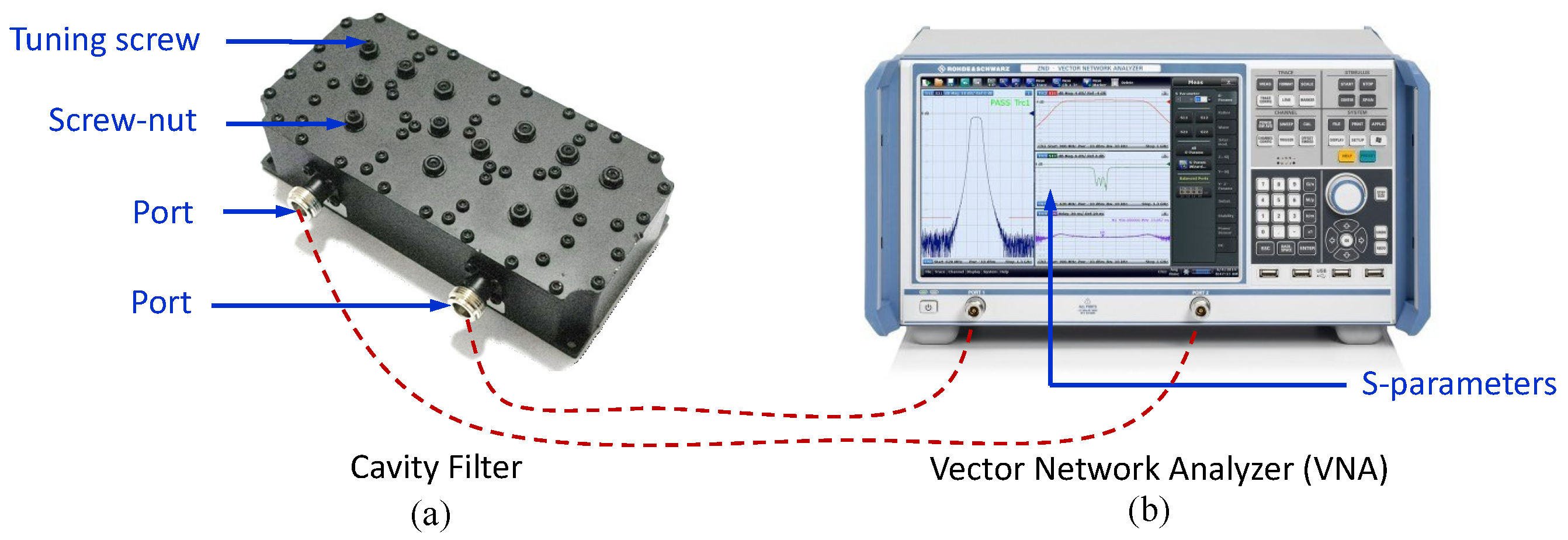
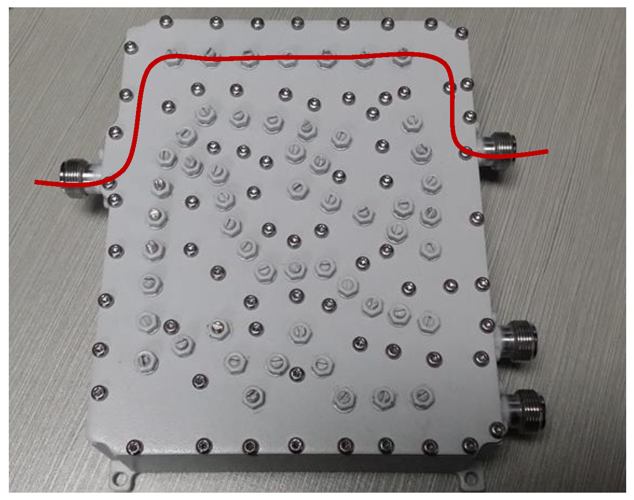
The cavity filter is a metal device for filtering signals and suppressing noises, which is often used in microwave, satellite, radar, electronic countermeasure (ECM), and various electronic testing devices. A cavity filter is mainly composed of cavities with resonators, inserted tuning screws, locking screw-nuts, and a covering plate; see 
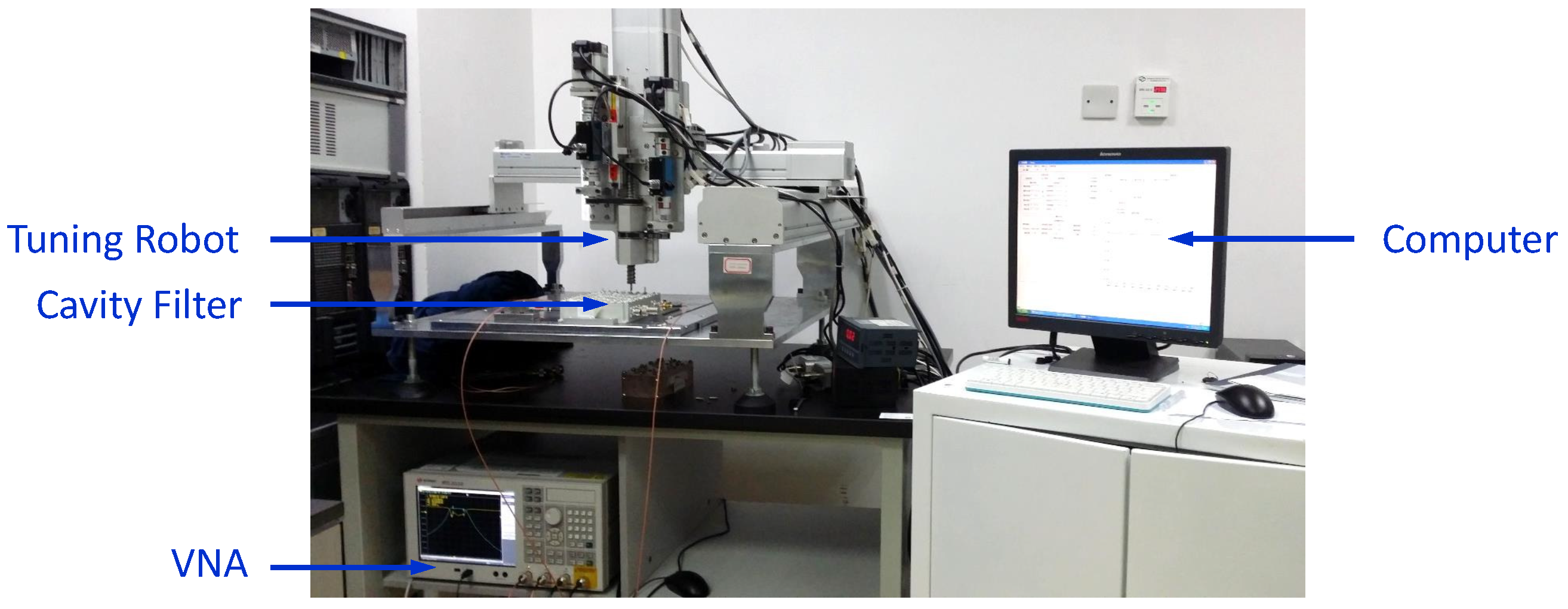
Figure 1a. A cavity filter is a product that passes or eliminates microwave signals in specific frequency bands. Due to high working frequencies and inevitable manufacturing errors, unfortunately, almost every cavity filter product needs to be manually adjusted to meet its design specifications. During the tuning process, the measured cavity filter is connected to a Vector Network Analyzer (VNA) (
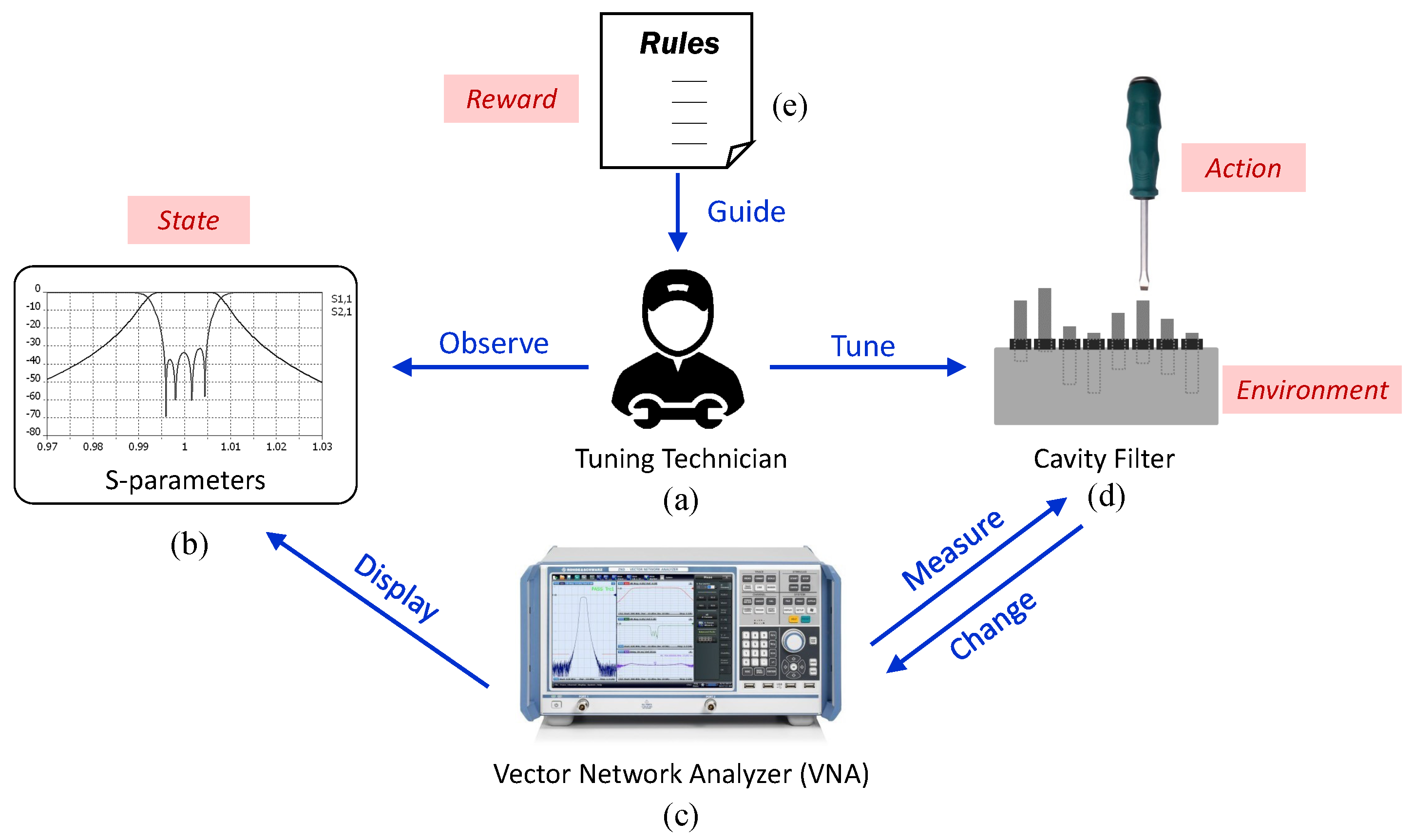
Figure 1b) and iteratively adjusted by a technician with a screwdriver. Almost every inserted screw will be tuned according to the S–parameter curves shown in the VNA. The curves indicate the current tuning state of the product and give guidance to the tuning technician to perform the next action such that the curves are gradually optimized until reaching the desired targets. Figure 2 shows the overall manual tuning process.
There are numerous possible difficulties during the task of cavity filter tuning. First, the relations between tuning screws and S–parameters would be complex. Theoretical analysis does not ensure validity since the manufacturing errors are not considered. In fact, each screw has its physical function in adjusting the S–parameter curves, but the actual product differs a lot from the designed pattern. Second, the cavity filter products have the feature of small-batch multiple varieties, which means that the tuning strategy for one filter category is not necessarily valid for another, even though they may have similar structures or tuning elements. Even for the same product type, differences would be obvious between individuals. Therefore, it is futile to simply copy the inserted screw positions of a tuned filter to a detuned one.
The above challenges make experienced technicians very critical. These “experts” are usually trained for several months to master the tuning strategies before they can handle real tuning tasks. An untrained person may get lost in the mazelike tuning task and never reach the target. On the basis of our investigations, experienced tuning technicians differ in two aspects from ordinary people with no experience. The first significant difference is that experienced technicians can accurately identify and evaluate the current situation, i.e., whether a curve’s change is good or bad. This is the foundation of all success. On this basis, they are also expertized in mastering the tuning amount. In other words, they know which screw to tune, and to what extent. However, all of these experiences are usually perceivable but indescribable.
To automate the tuning process, a powerful and stable automated tuning robot is essential. More importantly, a tuning algorithm should be designed that can accurately provide a tuning strategy at each tuning stage to successfully tune the filter as quickly as possible. In previous studies, automatic tuning methods based on time-domain response [3], model parameter extraction [4], and data-driven modeling techniques (i.e., Neural Network [5], Support Vector Regression [6], fuzzy logic control [7], etc.) have been investigated; however, these methods either rely heavily on individual product models or require data collection, and have limited generalization capabilities. In this work, we still focus on the tuning algorithm but pay more attention to the autonomy of the algorithm. To easily implement the algorithm, a computer-aided tuning robot system has also been developed, but the details are not the focus of this article.
As a breathtaking achievement in recent years, Reinforcement Learning (RL) has attracted extensive attention worldwide. From the perspective of bionics and behavioral psychology, RL can be seen as a manipulation of the conditioned reflex. Thorndike proposed the Law of Effect, which indicates that the strength of a connection is influenced by the consequences of a response [8]. Such a biological intelligence model allows animals to learn from the rewards or punishments they receive for trying different behaviors to choose the behavior that the trainer most expects in that situation. Therefore, the agent using RL is able to autonomously discover and select the actions that generate the greatest returns by experimenting with different actions. Intuitively, the manual tuning process is very similar to RL in many ways. To tune the screws of a cavity filter is equivalent to exploring the environment while watching the S–parameters curve from the VNA, which relates closely to obtaining environmental observations. The reward is instantiated in the personal evaluation of the current situation. For these reasons, plenty of studies have exploited RL for automatic tuning [9]. In this work, we utilize an actor–critic RL method to search for the optimal tuning policy.
Compared with the related work, the contributions of this paper are as follows. First, instead of simply fitting the screw positions to the S–parameters curves, we paid more attention to the process of tuning. In particular, the cavity filter tuning problem was formulated as a continuous RL problem and an effective solution was proposed based on Deep Deterministic Policy Gradient (DDPG). Second, we appropriately designed a reward function inspired by the experienced tuning processes, which stabilizes and accelerates the RL training. The proposed method was tested on a real cavity filter tuning issue and positive results were received. Third, we presented a framework to transfer the learned tuning policy to a new detuned product individual of the same type. With limited steps of exploration on the new product, a data-driven mapping model was built, and the relationship between the new and the old product could be learned. With this framework, the policy learned from RL can be generalized.
The remainder of the article is structured as follows. Section 2 introduces the tuning method of cavity filter and the basic principles of RL. In Section 3, our approach to autonomic tuning using continuous reinforcement learning is developed and presented. We first illustrate the framework of the algorithm and then explain the reward shaping through human inspirations. We also consider the generalization issue to make the algorithm more adaptable. A set of simulation experiments are carried out and the results to verify the validity of the framework are given in Section 4. In Section 5, some relevant issues are discussed in depth. Finally, Section 6 concludes the paper and makes a plan for future work.

2. Related Work

2.1. Automatic Cavity Filter Tuning

Research on automatic tuning algorithms has been going on for a long time. Studies in [3,10] utilized the time-domain response of the input reflection characteristics of the filter. This technique requires an optimal response as a template and relies on accurate estimates of features, which is not realistic in some cases. A sequential adjusting method based on Group Delay was proposed by [11]. This technique depends on the hypothetical computation of the group delay for each resonator. Notwithstanding, when processing the group delay of some resonator, other resonators should be short-circuited, which is infeasible in practice. Other methods based on model parameter extraction [4], poles and zeros [12], coupling matrix decomposition and extraction [13], etc. are also theoretical but almost invalid in most practical cases.
Another set of technologies utilize state-of-the-art artificial intelligence. Michalski proposed a novel tuning strategy building a data-driven model for the cavity filter product [5]. A feed-forward neural network was constructed to model the relationship between S–parameters and the screw deviations Δ Z , i.e., to train a nonlinear mapping f : S Δ Z . When tuning a detuned filter, the model is used to predict the screw deviations so that the desired S–parameters are approximated. Similarly, Zhou et al. exploited Support Vector Regression (SVR) to construct metamodels between screw rotations and coupling matrix change [6,14]; the screw rotations are not measured but obtained from two optimization procedures, and the calculation of coupling matrix also brings uncertainties. Furthermore, fuzzy logic control [7,15], neural-fuzzy control [16], Extreme Learning Machine (ELM) [17], and regularized deep belief network (R-DBN) [18] have also been applied in modeling cavity filters. These data-driven methods learn models simply from pregathered data without analyzing the complex theoretical and physical characteristics of the filter product, eliminating the error produced by the difference between the ideal model and the real product. However, these data-driven modeling techniques have constraints in generalization. In other words, to build a data-driven model of a cavity filter, a large number of data pairs should be collected; further, for every filter product type, data pairs should be recollected. Furthermore, the trained model cannot always adapt to the difference between individuals of the same product type, which limits the practicability. Wu et al. proposed new methods by integrating intelligent algorithms with filter theories, which also had good tuning effects [19,20], but the essence of the method is still fitting the screw and the scattering parameters, which might have the same problem as previous methods.
Different from the literature, we do not focus on any specific cavity filter model but make more efforts to study the tuning process. The tuning process of an expert is a typical exploration and exploitation process. The tuning expert interacts with the environment by adjusting the screws and observes the resulting S–parameter curves from the VNA. Then, a new tuning action is taken and the S–parameters are changed accordingly. Iterations are repeated until the filter is fully tuned. In [9], reinforcement learning (RL) approach was first tried to model the tuning process in the framework of Deep Q-Learning (DQN). However, this work only considered two screws, and the action was discretized for Q-learning. In [21], a novel automatic fine-tuning approach using DQN was proposed for planar bandpass filters. A forward model was trained by supervised learning to construct the environment and then interact with the agent in a DQN setting. As an improvement of DQN in handling with continuous state and action spaces, DDPG has been applied for tuning cavity filters with more tuning elements [22]. In [23], a new learning algorithm called Deep Imitation-Reinforcement learning for Tuning (DIRT) was proposed. By using the policy learned from behavior cloning, DIRT improved the performance of DDPG.
Based on the past achievements, in this work, we also explore the extension of RL algorithms in the tuning task with a carefully-designed reward function to accelerate training.

2.2. Reinforcement Learning and Reward Shaping

Reinforcement learning (RL) is a highly intelligent machine learning method. It does not rely on specific supervision, but purely on the learning strategy of starting from scratch by exploring the environment. RL has been proposed and created for some time, and more and more application domains see the key role of RL. However, most RL algorithms are still in their infancy and show very limited possibilities for real-world practical tasks. The high dimension of action space and state space and the difficulty of convergence hinder the development of RL. Represented by Deep Q-Learning (DQN), the combination of deep learning and RL has changed these. DQN uses a deep structure for value function approximation and designs two important techniques called the Experience Replay and the Target Network to make the learning more stable [24,25]. Since then, the study in [26] proposed DDPG algorithm to handle continuous action spaces. In DDPG, the Experience Replay and the Target Network are preserved from DQN, but DDPG uses the actor–critic mechanism for simultaneously updating a policy network and a value network.
RL is always time-consuming. In most practical situations, finding the optimal strategy through a lot of trial and error is unacceptable. In addition, it is important to evaluate the agent’s behavior during exploration. Since the RL algorithm only updates the strategy according to the reward, the definition of the reward function is of great concern. Reward shaping provides a solution by shaping an additional reward that is often designed by human experts or extracted from human demonstrations. Ng proposed an efficient potential-based reward shaping function and proved that it would not affect the convergence to the optimal policy [27,28]. Long-term studies have been conducted in shaping with human advice or demonstrations [29,30,31].
In this work, we designed a shaping reward inspired by experienced human tuning processes. In particular, the shaping term evaluates the tuning performance according to the changing trend of the S–parameters curve. Therefore, an instant reward will be obtained at each training step, and the reward will not be sparse anymore; thus, the learning is accelerated.
As a whole, the method proposed in this work is also based on RL, which means we consider the tuning process rather than the filter model. Furthermore, we consider effective ways to improve the performance of RL in accelerating and transferring.

3. Intelligent Tuning Based on DDPG

3.1. Preliminaries

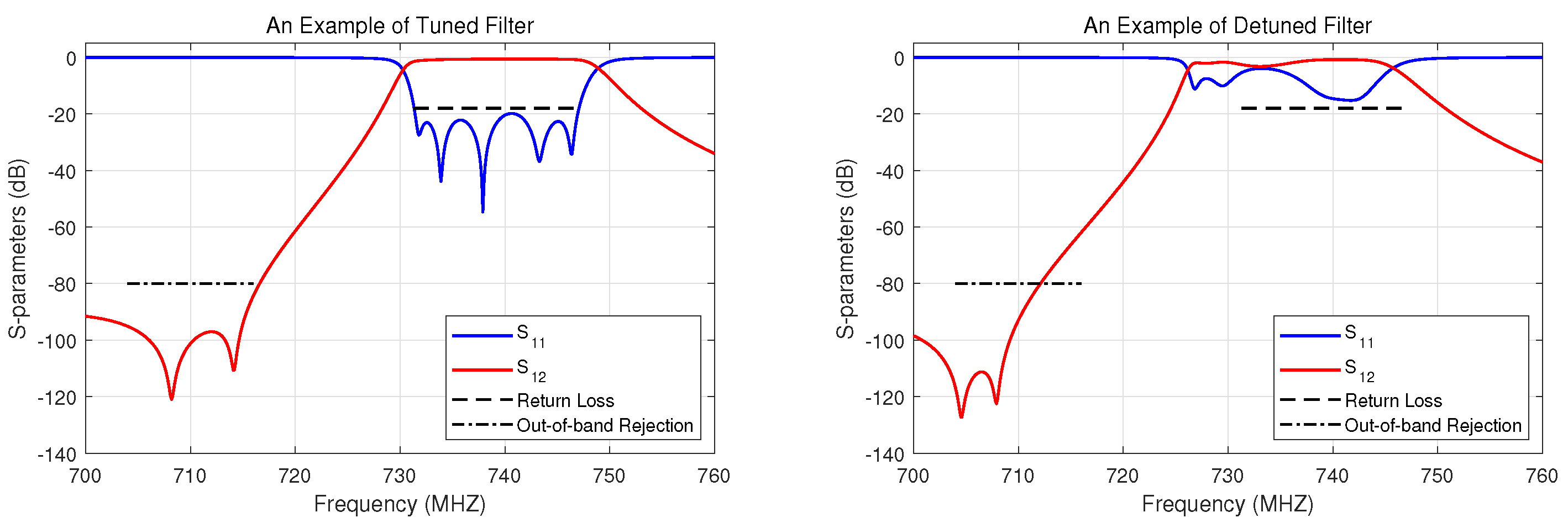
The observed states from the VNA are S–parameters curves, as shown in 
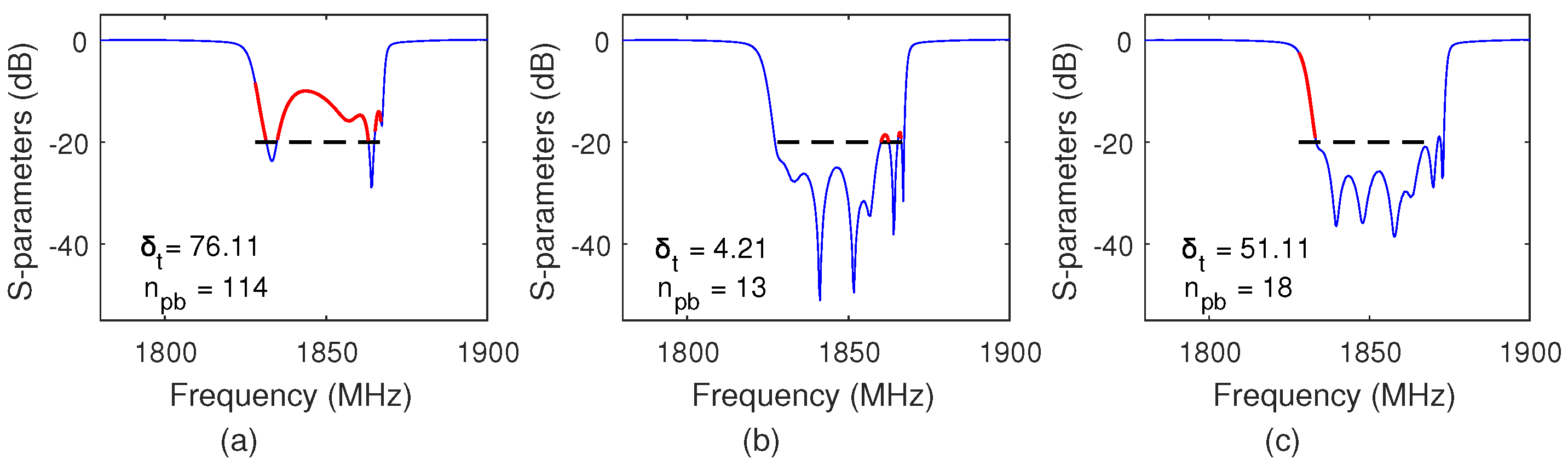
Figure 3. Since the cavity filter is a passive device, all signals passing through it come from external sources. During the test, the cavity filter device under test (DUT) is connected to a VNA through input/output ports. The VNA then sends the signal to the DUT to observe the received signal in the form of scattering parameter, or S–parameter for short. To meet the designed requirements of a cavity filter product, it is necessary to examine some test data, including the Return Loss, the Insertion Loss, the Pass-band Fluctuation, and the Out-of-band Rejection. S i j is the common notation of S–parameters, indicating the energy measured at port i injecting to port j. The return loss of port 1 is represented by S 11 , indicating the energy measured at port 1 after injecting from port 1 and returning to port 1. Similarly, the insertion loss of port 1 is always represented by S 12 , representing the energy measured at port 1 after injecting from port 1 to port 2 and returning to port 1. It is always required that the value of the return loss should be minimized within the passband (always less than or equal to 20 dB). In other words, the values of S 11 in Figure 3 must be under the black dashed benchmark line within the specified frequency range. For insertion losses, the value should be maximized within the same passband (always close to 0 dB).
In this work, we only consider the value of return loss, namely, the S 11 curve in the passband, as the state of RL, and ignore the other specifications, such as insertion loss. Therefore, the goal of tuning is to adjust the screw to control the S 11 curve to the target line. It is important to note that our tuning method can be applied to any filter class of radio frequency (RF) devices, including cavity filters, combiners, duplexers, and multiplexers.

3.2. Formulations

The RL method in this work follows the basic Markov Decision Process (MDP) settings. At each time step t, the agent observes a state s t from the environment. Then, it takes an action a t to interact with the environment and the state of the agent is transferred to s t + 1 . At the same time, the reward r t reflecting the current state and action pairs is obtained from the environment or specified by a human teacher. With the transition set ( s t , a t , r t , s t + 1 ) , the agent learns the policy with some optimization process, so that the expected future reward is maximized.
In our previous work, the framework of DQN was applied. A value function Q is defined based on the Bellman equation to compute the expected future reward. Then, the optimal action to take at each time step is the one that maximizes the Q values,
Q s t , a t = r t + γ max a t + 1 Q s t + 1 , a t + 1 ,
where s t , a t , and r t are the state, action, and reward, respectively, at step t; γ is a discounting factor. In DQN, a replay memory D is used to save transition sequences state, action, reward, new state. At each time step, a minibatch of transitions will be randomly selected from the replay buffer D for training the Q–network by minimizing the distance between the target Q-network and the current hypothesis model:
min θ y i Q s i , a i θ ,
where the target is
y i = r i + γ max a Q ^ s i + 1 , a ; θ .
Instead of using Deep Convolutional Neural Networks to approximate the value function, we extracted a feature set from the original S–parameters as the state. We follow the Experience Replay and the Target Network of DQN to ensure the stability of the algorithm. We also used the Euclidean distance between the S–parameters curves as a reward function. In particular, if the current curve is getting closer to the target, the reward is large, and vice versa. This definition of this reward is somewhat coarse and should be modified in the light of human experience.
In this work, the tuning algorithm is based on another important RL framework—DDPG—in which continuous actions are valid. Experience replay and Target Q-Network are preserved from DQN. DDPG is based on the actor–critic mechanism, where a critic function Q ( s , a ) and an actor function μ s θ μ are parameterized by two separate neural networks. The actor network is also called the policy network, which updates the policy with policy gradient. The critic network is similar to the value function in Q-learning, which evaluates the action from the actor network by updating the Q-values [26].
We define the tuning task as an MDP with the following settings. At each time step t, the agent is in a state s t S . In the tuning problem, the state s t is defined as the S–parameters ( S 11 ) curve (or some extracted features) drawn from the VNA. The agent performs an action a t A at each time step t to transfer state s t to a new state s t + 1 . The action is defined as the tuning amount we can take, i.e., the adjustment of each screw element. Unlike our previous work [9], screw lengths are continuous values instead of discrete values, which is more accurate and reasonable. Thus, the action at any time step can be represented as a vector of dimension m, where m is the number of valid tuning screws. The reward function consists of three parts, which take into account the process of tuning target and human experience.
The main algorithm is concluded in Algorithm 1. For details of the DDPG algorithm, readers can refer to [26].

3.3. Reward Shaping Inspired by Human Knowledge

After taking the action a t , a reward r t will be obtained. The value of the reward is an evaluation of the action taken, and the goal of RL is to learn a policy π ( s ) a so that the expected future reward is maximized. In some cases, the reward value can be derived directly from interaction with the environment, such as playing Atari games. In other cases, the reward function should be defined manually, such as the self-driving problem. Other tasks have reward functions that are difficult to define, such as robot manipulations. In these cases, the reward is always learned by demonstration. In this work, we use the experience of human tuning to manually design the reward function to make RL have better performance.
The reward r t of each step consists of three parts. r t goal directly describes the cost of each step taken by an action. Any step other than reaching the goal is rewarded with 0.01 . If the action results in an eligible S–parameters curve, i.e., reaching the tuning target, the reward will be added by + 10 .
r t goal s t , a t , s t + 1 = r target if s t + 1 = s goal r penalty otherwise .
Algorithm 1 Intelligent Tuning Based on DDPG
1:  Randomly initialize critic network and actor network with weights Q s , a θ Q and μ s θ μ .
2:  Initialize the target network Q and μ with the same weights as above.
3:  Initialize the replay buffer D.
4:  Randomly initialize inserted screw positions.
5:  for episode = 1,M do
6:     Read S–parameters from the VNA and formulate the initial state s 1 .
7:     for step = 1,T do
8:         Select action a t according to the current policy and exploration noise.
9:         Tune corresponding screws to execute action a t and compute reward r t , and observe new S–parameters to formulate new          state s t + 1 .
 
10:         Store the transition ( s t , a t , r t , s t + 1 ) in D.
11:         Sample a random minibatch of N transitions ( s i , a i , r i , s i + 1 ) from D.
12:         Set y i = r i + γ Q s i + 1 , μ s i + 1 θ μ θ Q .
13:         Update the critic network by minimizing the loss: L = 1 N i = 1 N y i Q s i , a i θ Q 2 .
14:         Update the actor network using the sampled policy gradient: θ μ J 1 N i = 1 N a Q s , a θ Q s = s i , a = μ s i θ μ μ s θ μ s i .
15:         Update the target networks:
            θ Q τ θ Q + 1 τ θ Q θ μ τ θ μ + 1 τ θ μ
 
16:     end for
17:  end for
To impose a penalty for one or more screws exceeding the length limit, a total reward of 0.1 is added. More specifically, if the action causes the screw to exceed its limit, the screw will remain unchanged and the agent will be rewarded with 0.1 / m , where m is the number of valid screws. The reward r t limit is formulated as
r t limit s t , a t , s t + 1 = 0.1 m · i = 1 m 1 z t + 1 ( i ) z max ( i ) , + , z min ( i ) ,
where 1 [ · ] is the indicator function with
1 x = 1 if x is True 0 otherwise ,
and z t ( i ) denotes the insertion position of the i-th tuning screw at the time step t. z max ( i ) and z min ( i ) denote, respectively, the maximum and minimum insertion position of the i-th screw.
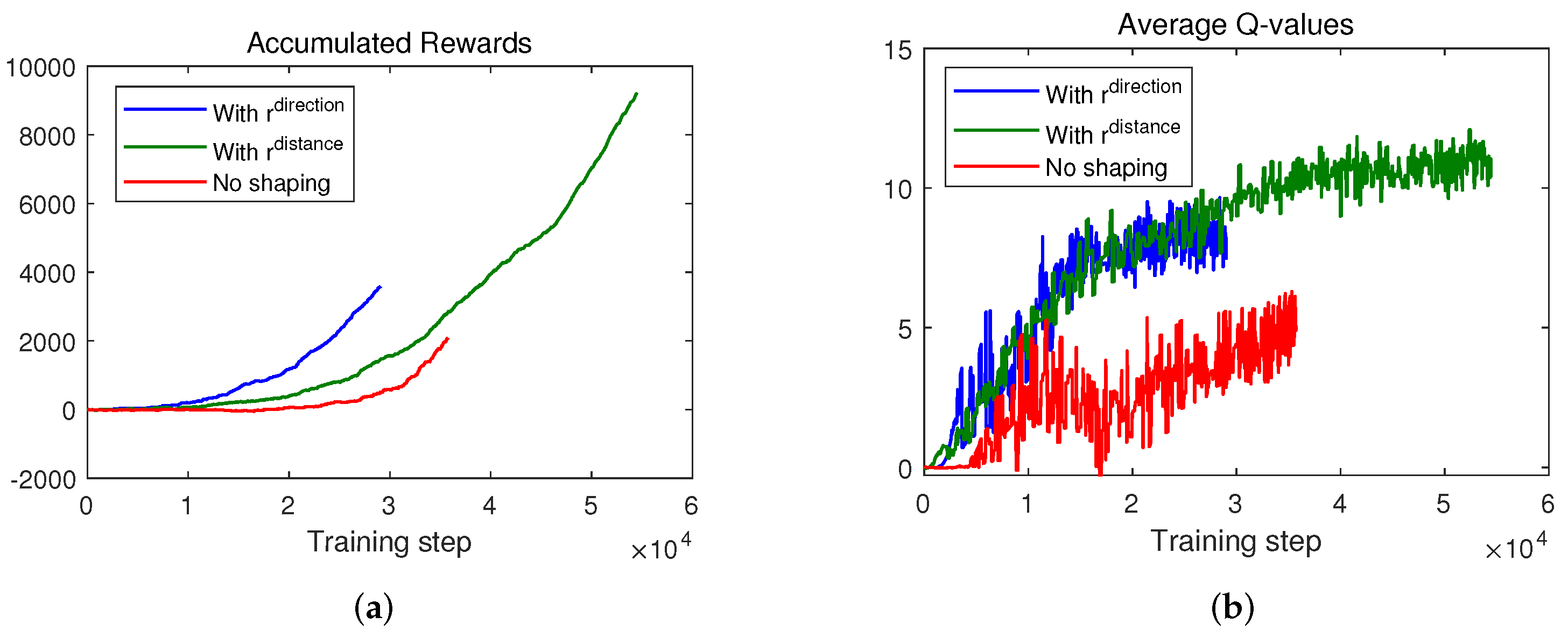
The third part is the most important reward r t direction 
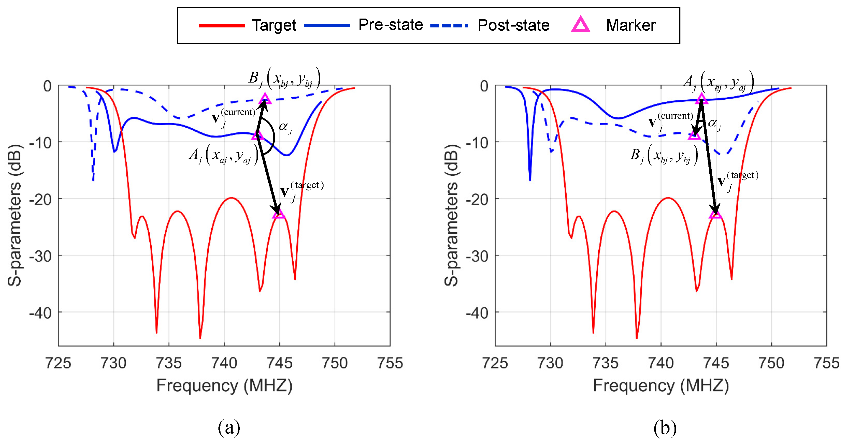
, which is formed in the evaluation of transitions from the current state to the next state, inspired by human tuning experience. Take into account the experienced tuning process. Technicians are able to optimize the S–parameters curve because they can evaluate changes to the curve. In other words, they do their best to make the S–parameters curve always move in the right direction. Therefore, the change direction of the S–parameters curve to the new curve can be expressed as a set of vectors. Each S 11 curve is truncated first, leaving only the central core area. The two curves are then discretized into the same number of sampling points. Thus, the vectors connecting two corresponding points of the curves can form a vector field. See Figure 4 for more details. In Figure 4a, the vector v j ( current ) represents the moving direction of the point A j on the blue curve (current state) to the point B j on the green dashed curve (a new state).
v j ( current ) = x b j x a j y b j y a j .
Similarly, to represent the changing direction of a curve to a target line, a set of vectors connecting each two corresponding points on the curve and the target line can be applied, as shown in Figure 4, denoted by v j ( target ) .
Therefore, we can use the sum of each cosine value of the angle α j between v j ( current ) and v j ( target ) to calculate the directional difference of two S–parameters curves, i.e.,
cos α j = v j ( current ) · v j ( target ) v j ( current ) v j ( target ) ,
where
α j = v j ( current ) , v j ( target ) .
The intuition to use cosine values is pretty simple. In order to adjust screws to maximally drive the current S–parameters curve to reach the target, we want each point on the curve to move as far as possible toward the goal. The cosine value of two vectors within the range [ 1 , 1 ] describes the similarity between the current direction and the target direction. The closer the current vector is to the target, the higher the value. More specifically, the cosine value of angle α j in Figure 4a is larger than 0 because α j is less than 90 , representing that v j ( current ) and v j ( target ) almost share the same direction. Conversely, the value of angle α j in Figure 4b will be less than 0 since α j is larger than 90 , which indicates that the two vectors have opposite directions. Therefore, the third shaping reward is formulated as
r t direction s t , a t , s t + 1 = j = 1 n cos α t , j ,
where
cos α t , j = v j ( t ) · v j ( target ) v j ( t ) v j ( target ) ,
in which v j ( t ) denotes the vector connecting the point j on the S 11 curve before and after tuning at time step t.
The cosine value only describes the direction of movement of each point on the curve. In addition, the length of each vector represents the extent of the movement. So, we multiply the cosine value by the moving amount of that point in the target direction. Therefore, the human-experience-shaped reward can be improved by
r t direction s t , a t , s t + 1 = 1 n j = 1 n v j ( t ) v j ( target ) · cos α t , j .
Therefore, the generated shaping reward inspired by human experience naturally shows the overall degree to which the curve changes in the direction of the target. The overall reward function is the sum of these three parts:
r t + 1 = λ 1 · r t + 1 goal + λ 2 · r t + 1 limit + λ 3 · r t + 1 direction ,
where λ 1 , λ 2 , and λ 3 are weights for a trade-off.

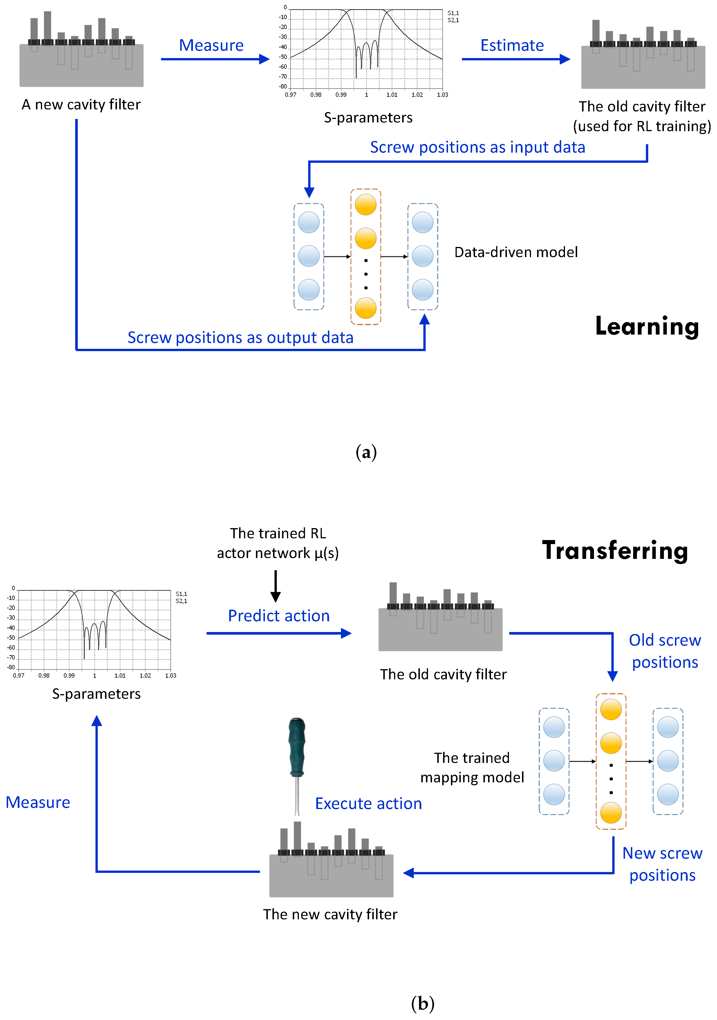
3.4. Generalize the Learned Policy

To learn how to tune a filter with RL is only a first and basic step. Since RL training always takes a long time to converge, and every product individual is different, how to adapt the individual differences is a challenging issue. If the trained policy cannot be generalized, RL loses its significance and will have no more advantage than supervised learning. In this work, we present a framework to tackle the generalization problem after RL training. Specifically, our aim is to tune a new detuned cavity filter to its target within as few steps as possible, after RL training on a benchmark product of the same type.
The framework contains two phases: learning and transferring. In the learning phase, we randomly explore the new filter product, collect enough data pairs, and build a data-driven mapping model between the new filter product and the old one. To achieve this, an inverse estimation model needs to be first built, i.e., a mapping from the S–parameters to the screw positions of the old filter product. The inverse estimation model could be built with data examples collected during the RL training process. Once we have a new product individual, we first randomly place the screws and record their corresponding S–parameters curves. Then, the inverse estimation model is used to predict the screw positions on the old filter product (which has already been trained). Finally, the two sets of screw data are used for constructing the data-driven mapping model. The learning phase is concluded in Figure 5a.
In the transferring phase, the learned data-driven mapping model is used to transfer the trained RL policy to the new product. When connecting the new product to the VNA, S–parameters could be measured. The trained RL policy network μ ( s ) predicts the best action to take. However, since the policy network is based on the old filter product, the predicted action cannot be directly applied. The mapping model learned in the learning phase should be used to transfer screw positions from the old to the new. The action on the new product is executed. The process is shown in Figure 5b.
It is worth noting that to build the inverse estimation model, data pairs including screw positions and S–parameters curves should be collected. Fortunately, the data could be collected at the same time with RL training. A way to correctly record screw positions is necessary.

4. Experiment

4.1. Settings

To evaluate the proposed tuning algorithm, simulation experiments are carried out on a four-screw cavity filter. Since frequent adjustment of screws on real products can cause damage to filter products and the tuning robot, we use a data-driven simulation model for experiments instead. The screw positions and S–parameters data collected randomly by the automatic tuning robot were used to build the model (Figure 6). In total, 2400 data pairs were collected. The robot tuning system is composed of a three-axis robotic arm, an industrial personal computer, and a control cabinet. Five servomotors are used for moving in the x, y, and z-direction, as well as the rotation for tuning the screw and the screw-nut. The robot can output specified rotation angles, so that desired tuning amount on the filter can be recorded. The S 11 curve is observed from the VNA as the state for RL. To calculate the shaping reward, the central region of the S 11 curve is first truncated. The cavity filter model is a combiner with four channels, and only one channel is considered for the test (Figure 7). The channel has four cavities with seven tuning screws, but for the sake of simplicity, only the tuning screws of four resonators are used in the experiment, indicating that the action dimension of RL is 4. Other screws remain in their standard position.
The DDPG model used in our experiments is similar to the low-dimensional network structure in [26]. We extracted the S–parameters into a 20-dimensional feature set with Principle Component Analysis (PCA) as the input to the value network (critic) and the policy network (actor). The output of the policy network was a 4-dimensional set of continuous actions, representing actions taken on four screws. Both networks are feed-forward neural networks with the extracted feature set as the input. Both of them have two hidden layers, with 300 units on the first hidden layer and 600 units on the second. The activation function for the two hidden layers is Relu, while the output layer uses tanh as the activation function. The learning rate is 0.0001 for the actor network and 0.001 for the critic network. Weights are randomly initialized. For the filter product we used, the effective screw insertion position values were normalized and limited to [ 3 , + 3 ] , representing the rotation performed to the screw from a standard position by [ 540 , + 540 ] degrees. For each tuning step, the action value output by the policy network is multiplied by a small size length to calculate the final tuning amount on each screw, i.e., the update of the screw positions would be
z t + 1 ( i ) : = z t ( i ) + a t ( i ) · Δ z ( i ) ,
where z t ( i ) is the position of the i-th tuning screw at time step t, a t ( i ) is the output action of the policy network at time step t, and Δ z ( i ) is a small step-size. The Δ z ( i ) of all four screws were set to the value of 0.25 in the experiment of this proposed work.
To avoid getting stuck, we only trained the DDPG model with a maximum of 200 steps per episode and tested the model after every four episodes. In other words, if the algorithm has already tuned the filter 200 times but the filter has not yet been fully tuned, this episode will be stopped. At the beginning of each episode, the screw insertion positions were randomly initialized. The ratios for the three reward terms were set with λ 1 = λ 2 = 1 , λ 3 = 10 . The ratio values were selected based on experience or practical tests. r target and r penalty were set to + 10 and 0.01 , respectively. Other parameter values related to RL training are listed in Appendix A.
To validate the effectiveness of the proposed, human-inspired reward shaping, three sets of experiments with different reward settings were conducted. The three cases are (1) with the human-inspired shaping reward r t direction , (2) with a Euclidean distance shaping reward r t distance , and (3) without any shaping reward. Specifically, r t distance measures the distance between the S–parameter values and the tuning target:
r t distance s t , a t , s t + 1 = 1 if δ t > δ t + 1 0 otherwise ,
where δ t is the Euclidean distance between the S 11 values and the return loss within the passband:
δ t = k = 1 n p b S 11 t , k R L 2 with S 11 t , k R L > 0 ,
where R L is the return loss target (e.g., 20 dB), n p b denotes the number of points sampled on the curve within the passband (only considering the points where S 11 > R L ). The reason to use r t distance for comparison is that the Euclidean distance is intuitive and simple for evaluating the curve state, and has been used in previous related work [9,22]; however, it has limitations in handling the horizontal shift of the curve, which will be analyzed later.
The algorithm was implemented in Python language and compiled in Anaconda. The environment of RL was a neural network model, pretrained by Keras in Anaconda with randomly collected data pairs. Some parameter values related to RL training are listed in Appendix A.

4.2. Results

Figure 8 describes the corresponding results in three cases, respectively. The figures on the left show the tuning steps during training, while the figures on the right show the tuning steps during testing (i.e., simply run after every four training episodes). The vertical axes show the number of tuning steps in each episode. At the beginning of the explorations, the agent can hardly make the filter be fully tuned in 200 steps. As the exploration goes on, the agent takes fewer steps to succeed. In other words, the fewer steps in one episode, the better; further, the fewer episodes used to converge, the better. When applying the knowledge-inspired shaping reward r t direction , the algorithm almost succeeded in finding the optimal tuning strategy in about 100 episodes. In contrast, using the Euclidean distance reward r t distance and without any shaping reward (i.e., r consists only of r goal and r limit ), it takes more than 250 episodes for the algorithm to converge to an optimal policy.
The results indicate the following: (i) By applying the DDPG algorithm with and without reward shaping, the cavity filter can both be fully tuned. This indicates that the proposed RL method is effective to learn how to tune a detuned filter to its target from scratch. (ii) By using a carefully prescribed shaping reward r t distance , the RL agent takes fewer episodes to converge to the optimal policy than using no shaping reward. This is because, without any shaping reward, the agent can only receive feedback when the cavity filter is finely tuned, which always takes a long period of time. On the contrary, adding an extra shaping reward provides instant feedback at each training step; thus, the total reward will not be sparse anymore and the learning is accelerated. (iii) An inappropriate shaping reward will not accelerate learning. Simply computing the Euclidean distance to the target for shaping the reward has no obvious advantage over without any shaping reward.
Although it seems reasonable to use the distance for evaluating the tuning state, it is not good at handling the cases when the S–parameters curve has a horizontal shift. Figure 9 illustrates the computation of the Euclidean distance of three different S–parameter curves. Only the points above −20 dB are considered for computing the distance, which have been marked red. In Figure 9a, the curve is shifted away from the target vertically. A total of 114 points are included for calculation, and the computed Euclidean distance is 76.11. In Figure 9b, the curve almost reaches the target, and only 13 points are included for calculation, with a final distance value of 4.21. In Figure 9c, the curve also seems to be approaching the target and only 18 points do not meet the requirement, but the corresponding distance value reaches 51.11, which is relatively high. Compared with the curve in Figure 9b, the shape of the curve in Figure 9c is almost the same, but has a slight shift to the right. This indicates that a small horizontal shift will cause a large distance value. Therefore, simply using the Euclidean distance for evaluating the reward is not always appropriate.
Figure 10 shows the learning curves of the RL process. Figure 10a shows the accumulated rewards. We can find that with knowledge-inspired reward r t direction or the Euclidean distance reward r t distance , the reward value is accumulated faster than without any shaping reward because the agent obtains shaping reward values more frequently, and a sparser reward value of + 10 will be added if the filter is successfully tuned. A steep rise in accumulated reward denotes a more frequently added + 10 . We also reserved a set of randomly obtained states and computed their average Q values after each training episode. The blue and green curve in Figure 10b increase more quickly and steadily than the red one, which also reflects the effectiveness of the shaping reward. However, when using r t distance , the total number of training steps reaches about 55,000, which indicates more failed episodes (i.e., 200 training steps have been fully used but the filter has not been fully tuned) during training. Therefore, using an inappropriate shaping reward does not accelerate training but reduces the exploration performance.
Some S–parameters curves are also obtained during the experiment. In Figure 11, the curves of S 11 for four different tuning processes are given. Most tuning tests could be finished in about 10 steps (depending on the starting position and the step size). As the target of RL is not a fixed S 11 but a range, the end states of the experiment are different in shape. In other words, the shape of the final curve does not matter. Any curve is acceptable as long as the value of S 11 in the passband is less than 20 dB.

4.3. Generalization Test

Finally, the generalization framework proposed in Section 3.4 was tested. We manually constructed new filter products based on the trained product by making alterations to the screw positions. Specifically, we linearly scaled each screw of the old cavity filter by multiplying with a set of factors [ 0.5 , 1.0 , 1.5 , 0.25 ] to simulate a new one. Then, the mapping model was learned as the learning phase described in Section 3.4. It is important to reduce the number of collected data pairs because frequently adjusting the screws on a new filter product should be avoided. We collected 50, 100, and 1000 data examples, respectively, on the new filter product for training and comparison. Afterwards, the trained mapping models Mapping 50, Mapping 100, and Mapping 1000 were applied directly in the transferring phase. At each tuning step, the action is predicted by the RL policy network and then mapped to the corresponding value in the new filter. Then, the mapped action is executed on the new filter product.
For each of the three models—i.e., Mapping 50, Mapping 100, and Mapping 1000—100 episodes with a maximum of 50 tuning steps in each episode have been tested. Figure 12 provides some test results. In Figure 12 (left), the number of tuning steps in each episode for each mapping model has been shown. Figure 12 (right) quantitatively compares the three mapping models. With Mapping 50 model, only in 65 episodes among 100 could the new constructed filter be successfully tuned, while with Mapping 1000 model, 82 episodes are target-reached. It is evident that with more training data, the new product could be more accurately transferred to the old trained model. In practice, to find a good trade-off between data size and performance should be carefully treated.
It should also be noted that, in this work, we simulate the new filter product by simply rescaling the screws of the old. However, constructing other kinds of differences should also be possible, such as by shifting or adding noises to screws of the old one. In practice, the differences between individuals could be more nonlinear and complicated, which is also another important topic to be studied in the future.

5. Discussions

It seems a fuss to use RL, since other methods, such as training supervised learning models [5,6,14,16,32] or to study the physical characteristics of the cavity filter [3,10,11,12], can still achieve the same goal; in most cases, those methods also do not need a large number of iterations. However, these methods always need a pretuned filter model as a benchmark or experienced tuning experts for guidance. In addition, they have weak potential in generalization. As explained in Section 1, cavity filters have a wide range of types, and they are different in structure and design specifications. Therefore, simply modeling one filter product may fail in adapting to others. In contrast, humans can learn strategies from experience and extract useful information for further use, no matter how the filter type changes. Therefore, it is more reasonable to study the tuning strategies rather than a cavity filter sample.
RL algorithms do not depend on any explicit guidelines or supervision but autonomously learn the tuning strategies from scratch. More importantly, the learned strategies are expected to be generalized to other cases, i.e., to different individuals of the same type or even totally different types. This work is an extension to [9,33]. In [9], DQN is used for the first time to solve the tuning problem but the state and action spaces are both very limited. In [33], DDPG first shows its effectiveness for tuning. The methods proposed in [21,22,34] also utilize DQN, double DQN, or DDPG, and based on previous studies, these works attempt more filter orders (screw numbers) or more elaborate reward functions, but have little consideration of generalization or transfer problems. In this work, we have considered the issue of transferring the learned knowledge, even though the differences between individuals are man-made, which does not necessarily accord with reality. Therefore, the problem related to generalization or transfer is still demanding work to be addressed in the future. It is also worth noting that some other methods such as Particle Filtering and Particle Swarm Optimization [35] can also be considered in our future work to focus on the tuning process.
Our current study is somewhat limited by the difficulty of the experiment. Although we have a robotic tuning system, it is not enough efficient, and thus, has not been directly used for executing RL training for safety reasons. Without an effective tuning machine, either a simulation model or manual tuning can be used for the experiment. By comprehensive consideration, we use the robot tuning system for collecting data pairs to build the simulation environment, then train the RL model in simulation.
Another popular way to integrate human experience with RL is to use imitation learning (also called learning from demonstration), which provides a straightforward way for the agent to master flexible policies. Studies in [36,37] integrate DQN and DDPG with human demonstrations by pretraining on the demonstrated data. However, this idea is somewhat hard for our task. First, in order to use demonstration data, a tuning expert should be always available, which is not guaranteed. Second, data acquisition is also important. The tuning action is continuous, and the tuning amount directly determines the change amount of the S–parameters. To record the demonstration data, both screw positions and S–parameters should be discretized; it also needs collaboration with tuning technicians. Finally, the recorded data might highly depend on the skills of the tuning technician. Different people perform differently, and even the same person may differ in the process of tuning the same product, which brings additional noise. Due to these reasons, imitation learning is currently not appropriate for this task. Instead of directly using human demonstration, we integrate human intelligence into the design of the reward function, which performs much better than simply learning from human demonstrated data.

6. Conclusions

Humans can handle plenty of complicated tasks that are difficult for robots. How to extract and learn from human strategies is a key issue for making robots more intelligent. Tuning cavity filters generally relies on the rules of thumb and can only be operated by highly skilled technicians. The automation of cavity filter tuning is a challenge. In this paper, the tuning task of cavity filters is defined as a continuous RL problem, and a possible solution for autonomous tuning is presented under the DDPG framework. We designed an appropriate reward function with a shaping term inspired by the human tuning experience. At any time, the S–parameters curve is driven in the desired direction as much as possible. We successfully verified our algorithm on a four-screw cavity filter product. The algorithm can adjust the filter to the desired target from any random starting position of the screw within a certain range of screw positions. We also proposed a framework for generalizing the trained policy on a new detuned product individual and tested its validity on products with simulated differences.
Nevertheless, the proposed method for automatically tuning cavity filters still needs to be extended. The filter model used in the experiment is simple and the curve always changes in the vertical direction. The environment used for DDPG training was a simulation model rather than a real product, which also leaves room for improvement. The simulation environment cannot be completely consistent with the real situation and cannot accurately reflect individual differences when tackling the generalization problem. One possible future direction is to try more tuning screws and a wider range of screw positions, with the help of a powerful tuning robot. Another future orientation is to continue to explore the transfer problem, which is to consider the transfer of learned skills to more complex but more practical new environments. It is also considerable to use domain randomization, i.e., to train the RL model directly on different filter models so that the generalization ability of the trained policy could be increased.

Author Contributions

Conceptualization, Z.W.; methodology, Z.W. and Y.O.; software, Z.W.; validation, Z.W.; formal analysis, Z.W.; investigation, Z.W.; resources, Y.O.; writing—original draft preparation, Z.W.; writing—review and editing, Z.W.; visualization, Z.W.; supervision, Y.O.; project administration, Y.O.; funding acquisition, Y.O. All authors have read and agreed to the published version of the manuscript.

Funding

This work was jointly supported by Key-Area Research and Development Program of Guangdong Province (2019B090915002), National Natural Science Foundation of China (Grants U1813208, 62173319, and 62063006), Guangdong Basic and Applied Basic Research Foundation (2020B1515120054), and Shenzhen Fundamental Research Program (JCYJ20200109115610172).

Institutional Review Board Statement

Not applicable.

Informed Consent Statement

Not applicable.

Data Availability Statement

Not applicable.

Conflicts of Interest

The authors declare no conflict of interest.

Appendix A

The parameter values for DDPG training in the experiment is provided in Table A1. We conducted several rounds of experiments and recorded the best set of parameter values we think. The concrete values are closely related to the selected cavity filter model. Since we only considered four tuning screws and the input states were not images, the exploration space was not necessarily huge. So the size of the replay buffer was set to 100,000. The explore rate and discount factor were set to 1 and 0.9 for an appropriate trade-off between exploration and exploitation. The number of steps in successful tuning episodes is usually around 20. So the maximum number of steps for exploration in each episode was set to 200, which is 10 times of 20.
Table A1. Parameter values.
ParameterValueDescription
BUFFER_SIZE100,000size of reply buffer D
N32size of minibatch
EXPLORE100,000frames over which to anneal epsilon
epsilon1explore rate
γ 0.9discount factor
M_train400training episode count
M_test100testing episode count
T200maximum steps

References

  1. Xu, S.; Liu, J.; Yang, C.; Wu, X.; Xu, T. A Learning-Based Stable Servo Control Strategy Using Broad Learning System Applied for Microrobotic Control. IEEE Trans. Cybern. 2021, 1–11. [Google Scholar] [CrossRef] [PubMed]
  2. Xu, S.; Ou, Y.; Wang, Z.; Duan, J.; Li, H. Learning-Based Kinematic Control Using Position and Velocity Errors for Robot Trajectory Tracking. IEEE Trans. Syst. Man Cybern. Syst. 2022, 52, 1100–1110. [Google Scholar] [CrossRef]
  3. Dunsmore, J. Tuning band pass filters in the time domain. In Proceedings of the 1999 IEEE MTT-S International Microwave Symposium Digest, Anaheim, CA, USA, 13–19 June 1999; Volume 3, pp. 1351–1354. [Google Scholar] [CrossRef]
  4. Harscher, P.; Vahldieck, R.; Amari, S. Automated filter tuning using generalized low-pass prototype networks and gradient-based parameter extraction. IEEE Trans. Microw. Theory Tech. 2001, 49, 2532–2538. [Google Scholar] [CrossRef]
  5. Michalski, J.J. Artificial neural networks approach in microwave filter tuning. Prog. Electromagn. Res. M 2010, 13, 173–188. [Google Scholar] [CrossRef] [Green Version]
  6. Zhou, J.; Duan, B.; Huang, J. Influence and tuning of tunable screws for microwave filters using least squares support vector regression. Int. J. Rf Microw. Comput.-Aided Eng. 2010, 20, 422–429. [Google Scholar] [CrossRef]
  7. Moreira-Tamayo, O.; Pineda de Gyvez, J.; Sanchez-Sinencio, E. Filter tuning system using fuzzy logic. Electron. Lett. 1994, 30, 846. [Google Scholar] [CrossRef] [Green Version]
  8. Thorndike, E.L. Animal intelligence: An experimental study of the associative processes in animals. Psychol. Rev. Monogr. Suppl. 1898, 2, i-109. [Google Scholar] [CrossRef] [Green Version]
  9. Wang, Z.; Yang, J.; Hu, J.; Feng, W.; Ou, Y. Reinforcement Learning Approach to Learning Human Experience in Tuning Cavity Filters. In Proceedings of the 2015 IEEE International Conference on Robotics and Biomimetics (ROBIO), Zhuhai, China, 6–9 December 2015; pp. 2145–2150. [Google Scholar] [CrossRef]
  10. HP Application. Simplified Filter Tuning Using Time Domain; Technical Report; HP Application: Santa Rosa, CA, USA, 1999. [Google Scholar]
  11. Ness, J.B. A unified approach to the design, measurement, and tuning of coupled-resonator filters. IEEE Trans. Microw. Theory Tech. 1998, 46, 343–351. [Google Scholar] [CrossRef] [Green Version]
  12. Hsu, H.T.; Yao, H.W.; Zaki, K.A.; Atia, A.E. Computer-aided diagnosis and tuning of cascaded coupled resonators filters. IEEE Trans. Microw. Theory Tech. 2002, 50, 1137–1145. [Google Scholar] [CrossRef]
  13. Das, R.; Member, S.; Zhang, Q.; Member, S. Computer-Aided Tuning of Highly Lossy Microwave Filters Using Complex Coupling Matrix Decomposition and Extraction. IEEE Access 2018, 6, 57172–57179. [Google Scholar] [CrossRef]
  14. Zhou, J.; Duan, B.; Huang, J.; Cao, H. Data-driven modeling and optimization for cavity filters using linear programming support vector regression. Neural Comput. Appl. 2013, 24, 1771–1783. [Google Scholar] [CrossRef]
  15. Miraftab, V.; Mansour, R. Computer-aided tuning of microwave filters using fuzzy logic. IEEE Trans. Microw. Theory Tech. 2002, 50, 2781–2788. [Google Scholar] [CrossRef]
  16. Kacmajor, T.; Michalski, J.J. Neuro-fuzzy approach in microwave filter tuning. In Proceedings of the IEEE MTT-S International Microwave Symposium Digest, Baltimore, MD, USA, 5–10 June 2011; pp. 2–5. [Google Scholar] [CrossRef]
  17. Wu, S. Parametric model for microwave filter by using multiple hidden layer output matrix extreme learning machine. IET Microwaves Antennas Propag. 2019, 13, 1889–1896. [Google Scholar] [CrossRef]
  18. Pan, G.; Wu, Y.; Yu, M.; Fu, L.; Li, H. Inverse Modeling for Filters Using a Regularized Deep Neural Network Approach. IEEE Microw. Wirel. Components Lett. 2020, 30, 457–460. [Google Scholar] [CrossRef]
  19. Wu, S.; Liu, C.; Cao, W.; Wu, M. A new method for hybrid diagnosis and tuning of coaxial cavity filter. In Proceedings of the 36th Chinese Control Conference, Dalian, China, 16–28 July 2017; pp. 9692–9696. [Google Scholar]
  20. Wu, S.; Cao, W.; Wu, M.; Liu, C. Microwave Filter Modeling and Intelligent Tuning. J. Adv. Comput. Intell. Intell. Inform. 2018, 22, 924–932. [Google Scholar] [CrossRef]
  21. Ohira, M.; Takano, K.; Ma, Z. A Novel Deep-Q-Network-Based Fine-Tuning Approach for Planar Bandpass Filter Design. IEEE Microw. Wirel. Components Lett. 2021, 31, 638–641. [Google Scholar] [CrossRef]
  22. Larsson, H. Deep Reinforcement Learning for Cavity Filter Tuning. Master’s Thesis, Uppsala University, Uppsala, Sweden, 2018. [Google Scholar]
  23. Lindståh, S.; Lan, X. Reinforcement Learning with Imitation for Cavity Filter Tuning. In Proceedings of the 2020 IEEE/ASME International Conference on Advanced Intelligent Mechatronics (AIM), Virtual Conference, 6–10 July 2020; pp. 1335–1340. [Google Scholar] [CrossRef]
  24. Mnih, V.; Kavukcuoglu, K.; Silver, D.; Graves, A.; Antonoglou, I.; Wierstra, D.; Riedmiller, M. Playing Atari with Deep Reinforcement Learning. In Proceedings of the 2013 Annual Conference on Neural Information Processing Systems (NIPS 2013) Deep Learning Workshop, Lake Tahoe, NV, USA, 5–10 December 2013; pp. 1–9. [Google Scholar]
  25. Mnih, V.; Kavukcuoglu, K.; Silver, D.; Rusu, A.a.; Veness, J.; Bellemare, M.G.; Graves, A.; Riedmiller, M.; Fidjeland, A.K.; Ostrovski, G.; et al. Human-level control through deep reinforcement learning. Nature 2015, 518, 529–533. [Google Scholar] [CrossRef]
  26. Lillicrap, T.P.; Hunt, J.J.; Pritzel, A.; Heess, N.; Erez, T.; Tassa, Y.; Silver, D.; Wierstra, D. Continuous control with deep reinforcement learning. In Proceedings of the 2016 International Conference on Learning Representations, San Juan, PR, USA, 2–4 May 2016. [Google Scholar]
  27. Ng, A.Y.; Harada, D.; Russell, S.J. Policy Invariance Under Reward Transformations: Theory and Application to Reward Shaping. In Proceedings of the Sixteenth International Conference on Machine Learning, Los Angeles, CA, USA, 27–30 June 1999; pp. 278–287. [Google Scholar]
  28. Ng, A.Y. Shaping and Policy Search in Reinforcement Learning. Ph.D. Thesis, University of California, Berkeley, CA, USA, 2003. [Google Scholar]
  29. Brys, T.; Harutyunyan, A.; Suay, H.B.; Chernova, S.; Taylor, M.E.; Nowe, A. Reinforcement learning from demonstration through shaping. In Proceedings of the International Joint Conference on Artificial Intelligence (IJCAI), Buenos Aires, Argentina, 25–31 July 2015; pp. 3352–3358. [Google Scholar]
  30. Harutyunyan, A.; Brys, T.; Vrancx, P.; Nowé, A. Shaping Mario with Human Advice ( Demonstration ). In Proceedings of the 14th International Conference on Autonomous Agents and Multiagent Systems (AAMAS 2015), Istanbul, Turkey, 4–8 May 2015; pp. 1913–1914. [Google Scholar]
  31. Wang, G.; Fang, Z.; Li, P.; Li, B. Shaping in Reinforcement Learning via Knowledge Transferred from Human-Demonstrations. In Proceedings of the 34th Chinese Control Conference, Hangzhou, China, 28–30 July 2015; pp. 3033–3038. [Google Scholar]
  32. Michalski, J.J.; Gulgowski, J.; Kacmajor, T.; Mazur, M. Artificial Neural Network in Microwave Cavity Filter Tuning. In Microwave and Millimeter Wave Circuits and Systems: Emerging Design, Technologies, and Applications, 1st ed.; John Wiley & Sons, Ltd.: Hoboken, NJ, USA, 2013; Chapter 2. [Google Scholar]
  33. Wang, Z.; Ou, Y.; Wu, X.; Feng, W. Continuous Reinforcement Learning with Knowledge-Inspired Reward Shaping for Autonomous Cavity Filter Tuning. In Proceedings of the 2018 IEEE International Conference on Cyborg and Bionic Systems, Shenzhen, China, 25–27 October 2018; pp. 53–58. [Google Scholar] [CrossRef]
  34. Sekhri, E.; Kapoor, R.; Tamre, M. Double Deep Q-Learning Approach for Tuning Microwave Cavity Filters using Locally Linear Embedding Technique. In Proceedings of the 2020 International Conference Mechatronic Systems and Materials (MSM), Bialystok, Poland, 1–3 July 2020; pp. 1–6. [Google Scholar] [CrossRef]
  35. Bi, L.; Cao, W.; Hu, W.; Wu, M. Intelligent Tuning of Microwave Cavity Filters Using Granular Multi-Swarm Particle Swarm Optimization. IEEE Trans. Ind. Electron. 2021, 68, 12901–12911. [Google Scholar] [CrossRef]
  36. Hester, T.; Vecerik, M.; Pietquin, O.; Lanctot, M.; Schaul, T.; Piot, B.; Sendonaris, A.; Dulac-Arnold, G.; Osband, I.; Agapiou, J.; et al. Learning from Demonstrations for Real World Reinforcement Learning. arXiv 2017, arXiv:1704.03732. [Google Scholar]
  37. Večerík, M.; Hester, T.; Scholz, J.; Wang, F.; Pietquin, O.; Piot, B.; Heess, N.; Rothörl, T.; Lampe, T.; Riedmiller, M. Leveraging Demonstrations for Deep Reinforcement Learning on Robotics Problems with Sparse Rewards. arXiv 2017, arXiv:1707.08817. [Google Scholar]
Figure 1. The overview of cavity filter tuning task: (a) A cavity filter with screws and screw-nuts to be tuned. (b) An R&S ZND Vector Network Analyzer (VNA) displays the S–parameter curves. Red dashed splines indicate cables for connecting the cavity filter device under test and the VNA.
Applsci 12 02409 g001
Figure 2. The process of manually tuning a cavity filter. The tuning technician (a) observes the S–parameters curve ( S 11 ) (b) as shown in a Vector Network Analyzer (c) and adjusts the screws inserted into the cavity filter with a screwdriver (d) based on his own experience and tuning strategies (e). The whole process is very much similar to a reinforcement learning problem.
Applsci 12 02409 g002
Figure 3. S–parameter curves: the states observed during tuning. In this example, the design specifications require that, within the passband (731∼747 MHz), the S 11 curve should be less than 18 dB (Return Loss), and the S 12 curve should be no less than 2 db (Insertion Loss). For the Out-Of-Band Rejection, it requires that the S 12 curve should be less than 80 dB within the range (704∼716 MHz). These are the targets for cavity filter tuning.
Applsci 12 02409 g003
Figure 4. Formulate the change of S–parameter curves with vector fields: (a) The angle α j is obtuse denoting that the current change direction is moving away from the target. (b) The angle α j is acute denoting that the current change direction is approaching the target.
Applsci 12 02409 g004
Figure 5. The policy generalization framework: (a) The learning phase: learning the filter mapping model. (b) The transferring phase: transferring the learned RL policy to a new individual with the mapping model.
Applsci 12 02409 g005
Figure 6. The automatic tuning robot system used for experiment.
Applsci 12 02409 g006
Figure 7. The combiner with four channels to be tuned in the experiment. The red spline denotes the channel used for experiment.
Applsci 12 02409 g007
Figure 8. Tuning steps of the training and test episodes in three different reward settings: (a) The knowledge-inspired reward. (b) The Euclidean distance reward. (c) Without any shaping reward. We conduct a test episode after every four training episodes. The maximum tuning step is set to 200 for both training and test episodes.
Applsci 12 02409 g008
Figure 9. Simply computing the Euclidean distance is not appropriate to evaluate the case when the S–parameters curve has a horizontal shift. The curve in (a) has the largest distance since the central part is far from the target line. The curve (b) has the smallest distance since only small portion of the points are above the target line. The S 11 curve in (c) has a slight shift to the right but the computed distance becomes relatively high. Red parts indicate the points involved in the calculation of r t distance .
Applsci 12 02409 g009
Figure 10. Analysis of the performance with learning curves: (a) Accumulated rewards during training episodes. (b) Q-values of the fixed set of states randomly initialized before training and evaluated after each training episode. Curves are recorded from one of the experiments for comparing the three reward functions but similar trends were observed from different experiments.
Applsci 12 02409 g010
Figure 11. Test experimental results of a trained model for the four-screw filter. The frequency passband is within the range of [ 883 , 956 ] MHz. The initial screw positions are randomly set. In most test episodes, the filter could be successfully tuned to meet the target in no more than 20 steps.
Applsci 12 02409 g011
Figure 12. Performance of the transfer framework. (Left) Test tuning steps of the three mapping models trained with 1000, 100, and 50 data pairs. (Right) Bar charts quantitatively show the results of the three mapping models.
Applsci 12 02409 g012
Publisher’s Note: MDPI stays neutral with regard to jurisdictional claims in published maps and institutional affiliations.

