
An Implementation of the HDBSCAN* Clustering Algorithm


Abstract
:Featured Application
Abstract
1. Introduction
2. Background and Literature Review
2.1. DBSCAN
2.2. HDBSCAN*
2.2.1. Other Methods
2.2.2. The HDBSCAN* Algorithm
| Algorithm 1: HDBSCAN* main steps. |
|
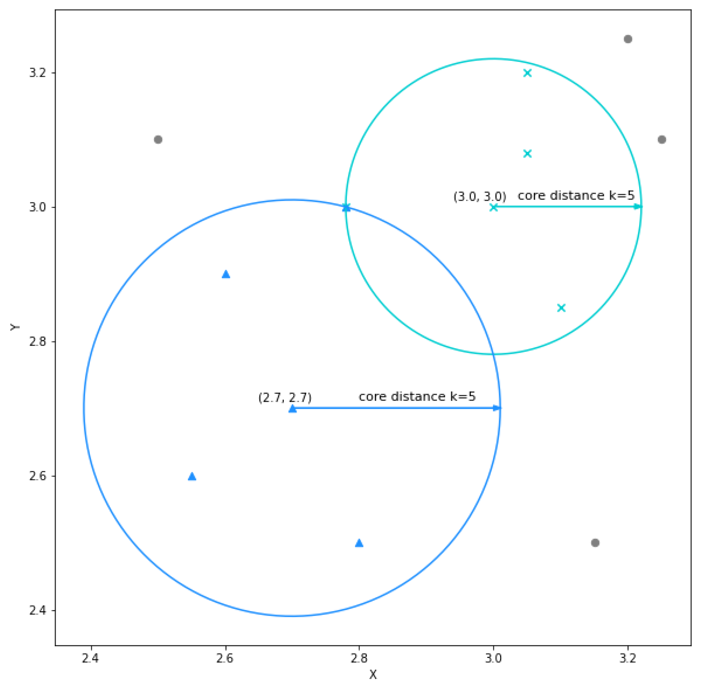
Compute the core distance for the k nearest neighbors for all points in the dataset; Compute the extended minimum spanning tree from a weighted graph, where the mutual reachability distances are the edges; Build the HDBSCAN* hierarchy from the extended minimum spanning tree; Find the prominent clusters from the hierarchy; Calculate the outlier scores; |
2.3. HDBSCAN* Implementations
2.3.1. Python HDBSCAN* Implementation
2.3.2. Java HDBSCAN* Implementation
- There are cases where important results are written to disk and subsequently read in again using customized file offset logic. Machine learning libraries do not commonly require access to the file system to persist results. Further, I/O can lead to performance issues;
- No unit tests. The reference implementation has no self-contained unit tests to verify the algorithm;
- There is some constraints functionality present in the reference implementation which adds complexity to several steps of the algorithm. This feature is not required;
- None of the logic leverages parallelization. There are several blocks of logic with high asymptotic complexity which could cause performance issues.
2.4. Tribuo Machine Learning Library
Tribuo Project Source Code
3. Materials and Methods
3.1. Study the HDBSCAN* Algorithm
3.1.1. The Theoretical Approach
3.1.2. The Practical Approach
3.2. Initial Development Phase
3.2.1. Add Unit Tests
3.2.2. Remove Unneeded File Input and Output
3.2.3. Remove Constraints Functionality
3.3. Review the Tribuo Project
3.4. Main Development Phase
3.4.1. Add the Tribuo Hdbscan Module
3.4.2. Implement the HDBSCAN* Core Logic
3.4.3. Develop a Novel Prediction Technique
| Algorithm 2: Compute cluster exemplars. |
 |
3.4.4. Add Concurrency
3.5. Compare the HDBSCAN* Implementations
3.5.1. Cluster Assignments and Outlier Scores
3.5.2. Predictions
3.5.3. Performance
4. Results and Discussion
4.1. Cluster Assignments and Outlier Scores
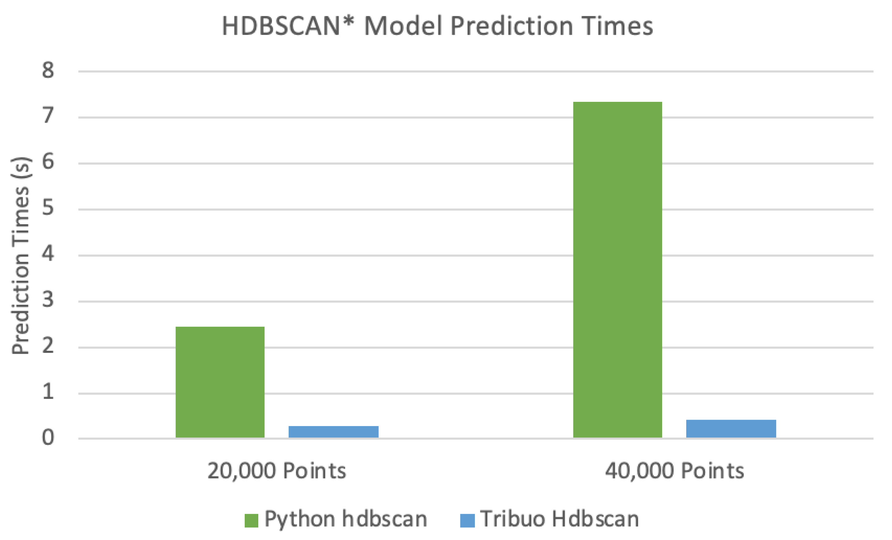
4.2. Predictions
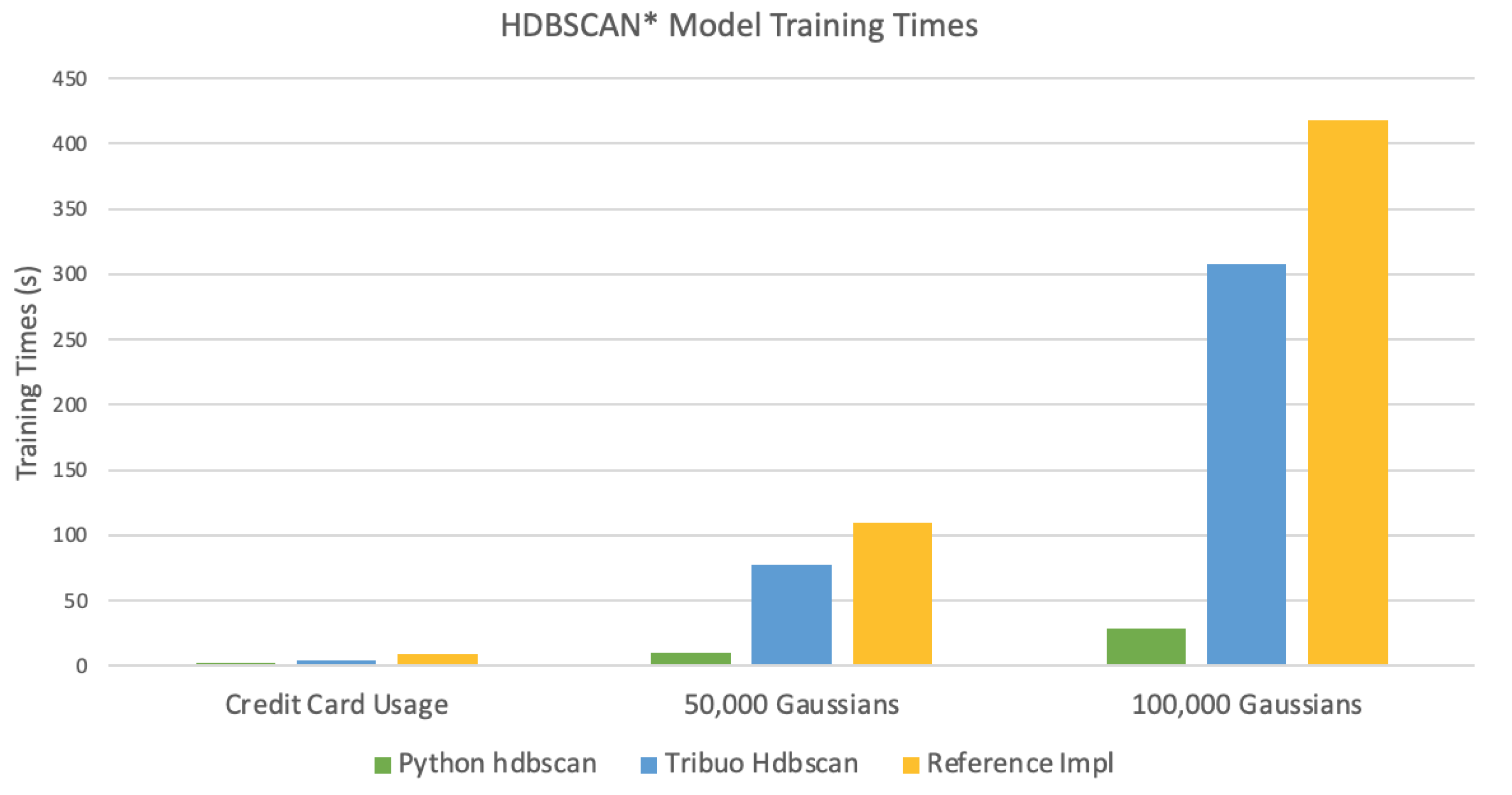
4.3. Performance
5. Conclusions and Future Work
Author Contributions
Funding
Institutional Review Board Statement
Data Availability Statement
Conflicts of Interest
References
- Al-sharoa, E.; Al-khassaweneh, M.A.; Aviyente, S. Detecting and tracking community structure in temporal networks: A low-rank+ sparse estimation based evolutionary clustering approach. IEEE Trans. Signal Inf. Process. Over Netw. 2019, 5, 723–738. [Google Scholar] [CrossRef]
- Al-Sharoa, E.; Al-khassaweneh, M.; Aviyente, S. Low-rank estimation based evolutionary clustering for community detection in temporal networks. In Proceedings of the ICASSP 2019–2019 IEEE International Conference on Acoustics, Speech and Signal Processing (ICASSP), Brighton, UK, 12–17 May 2019; IEEE: Piscataway, NJ, USA, 2019; pp. 5381–5385. [Google Scholar]
- Campello, R.J.; Moulavi, D.; Sander, J. Density-based Clustering Based on Hierarchical Density Estimates. In Advances in Knowledge Discovery and Data Mining, Proceedings of the Pacific-Asia Conference on Knowledge Discovery and Data Mining; Pei, J., Tseng, V.S., Cao, L., Motoda, H., Xu, G., Eds.; Springer: Berlin, Germany, 2013; pp. 160–172. [Google Scholar]
- McInnes, L.; Healy, J.; Astels, S. hdbscan: Hierarchical density based clustering. J. Open Source Softw. 2017, 2, 205. [Google Scholar] [CrossRef]
- Machine Learning in Java—Tribuo. Available online: https://tribuo.org/ (accessed on 24 July 2021).
- HDBSCAN* Clustering Tutorial. Available online: https://tribuo.org/learn/4.2/tutorials/clustering-hdbscan-tribuo-v4.html (accessed on 22 January 2022).
- Ester, M.; Kriegel, H.; Sander, J. A Density-Based Algorithm for Discovering Clusters in Large Spatial Databases with Noise. In Proceedings of the Second International Conference on Knowledge Discovery and Data Mining, Portland, OR, USA, 2 August 1996; pp. 226–231. [Google Scholar]
- Campello, R.J.; Moulavi, D.; Zimek, A.; Sander, J. Hierarchical Density Estimates for Data Clustering, Visualization, and Outlier Detection. ACM Trans. Knowl. Discov. Data (TKDD) 2015, 10, 5–56. [Google Scholar] [CrossRef]
- Ankerst, M.; Breunig, M.; Kriegel, H.; Sander, J. OPTICS: Ordering Points To Identify the Clustering Structure. In Proceedings of the 1999 ACM SIGMOD International Conference on Management of Data, United States, Philadelphia, PA, USA, 1–3 June 1999; ACM: New York, NY, USA, 1999; pp. 49–60. [Google Scholar]
- Maimon, O.; Rokach, L. Clustering methods. In Data Mining and Knowledge Discovery Handbook, 2nd ed.; Springer: Berlin/Heidelberg, Germany, 2006; pp. 321–352. [Google Scholar]
- Dinh, D.T.; Fujinami, T.; Huynh, V.N. Estimating the Optimal Number of Clusters in Categorical Data Clustering by Silhouette Coefficient. In KSS 2019: Knowledge and Systems Sciences; Chen, J., Huynh, V., Nguyen, G.N., Tang, X., Eds.; Communications in Computer and Information Science; Springer: Singapore, 2019; Volume 1103. [Google Scholar]
- McInnes, L.; Healy, J. Accelerated Hierarchical Density Based Clustering. In Proceedings of the 2017 IEEE International Conference on Data Mining Workshops (ICDMW), New Orleans, LA, USA, 18–21 November 2017; pp. 33–42. [Google Scholar]
- JavaVsPythonMLlibs. Available online: https://github.com/geoffreydstewart/JavaVsPythonMLlibs (accessed on 15 September 2021).
- Pedregosa, F.; Varoquaux, G.; Gramfort, A.; Michel, V.; Thirion, B.; Grisel, O.; Blondel, M.; Prettenhofer, P.; Weiss, R.; Dubourg, V.; et al. Scikit-learn: Machine Learning in Python. J. Mach. Learn. Res. 2011, 12, 2825–2830. [Google Scholar]
- Sia, W.; Lazarescu, M. Clustering Large Dynamic Datasets Using Exemplar Points. In Machine Learning and Data Mining in Pattern Recognition, Proceedings of the 4th International Conference on Machine Learning and Data Mining in Pattern Recognition, Leipzig, Germany, 18–20 July 2005; Springer: Berlin/Heidelberg, Germany, 2005; pp. 163–173. [Google Scholar]
- TribuoHdbscan. Available online: https://github.com/geoffreydstewart/TribuoHdbscan (accessed on 10 November 2021).
- IJava. Available online: https://github.com/SpencerPark/IJava (accessed on 22 September 2021).
- Credit Card Dataset for Clustering. Available online: https://www.kaggle.com/arjunbhasin2013/ccdata (accessed on 10 September 2021).
- Curtin, R.; March, W.; Ram, P.; Anderson, D.; Gray, A.; Isbell, C. Tree-Independent Dual-Tree Algorithms. In Proceedings of the 30th International Conference on Machine Learning, Atlanta, GA, USA, 17 June 2013; pp. 1435–1443. [Google Scholar]
- March, W.; Ram, P.; Gray, A. Fast Euclidean Minimum Spanning tree: Algorithm, Analysis, and Applications. In ACM SIGKDD International Conference on Knowledge Discovery and Data Mining, Proceedings of the 16th ACM SIGKDD International Conference on Knowledge Discovery and Data Mining, Washington, DC, USA, 24–27 July 2010; Association for Computing Machinery: New York, NY, USA, 2010; pp. 603–612. [Google Scholar]


| Algorithm | Strengths | Weaknesses |
|---|---|---|
| DBSCAN | Faster than the HDBSCAN* algorithm. | The algorithm requires an obscure, data dependent, distance parameter. |
| Discovers the clusters in a dataset. | Not effective at identifying clusters of varying density. | |
| Identifies outlier points. | ||
| HDBSCAN* | Identifies clusters of varying density | The algorithm has higher complexity compared to DBSCAN. |
| Discovers the clusters in a dataset. | ||
| Identifies outlier points. |
| Dataset Size | Number of Clusters | Exemplar Number |
|---|---|---|
| 100 | 5 | 12 |
| 2000 | 4 | 35 |
| 2000 | 8 | 39 |
| 5000 | 4 | 54 |
| 5000 | 8 | 60 |
| 9000 | 100 | 167 |
| 10,000 | 4 | 74 |
| 50,000 | 3 | 161 |
| 100,000 | 200 | 423 |
| Dataset | Ref Impl | Tribuo Hdbscan | Python hdbscan |
|---|---|---|---|
| 4 Centroids, 3 Features, 2000 points | 0.80 | 0.80 | 0.79 |
| 3 Centroids, 7 Features, 4000 points | 1.0 | 1.0 | 1.0 |
| Credit Card Data, 8949 points | N/A | N/A | N/A |
| Dataset | Tribuo Hdbscan | Python Hdbscan |
|---|---|---|
| 4 Centroids, 3 Features, 20 points | 0.87 | 0.87 |
| 3 Centroids, 4 Features, 1000 points | 1.0 | 1.0 |
| 5 Centroids, 4 Features, 1000 points | 1.0 | 1.0 |
Publisher’s Note: MDPI stays neutral with regard to jurisdictional claims in published maps and institutional affiliations. |
© 2022 by the authors. Licensee MDPI, Basel, Switzerland. This article is an open access article distributed under the terms and conditions of the Creative Commons Attribution (CC BY) license (https://creativecommons.org/licenses/by/4.0/).
Share and Cite
Stewart , G.; Al-Khassaweneh, M. An Implementation of the HDBSCAN* Clustering Algorithm. Appl. Sci. 2022, 12, 2405. https://doi.org/10.3390/app12052405
Stewart G, Al-Khassaweneh M. An Implementation of the HDBSCAN* Clustering Algorithm. Applied Sciences. 2022; 12(5):2405. https://doi.org/10.3390/app12052405
Chicago/Turabian StyleStewart , Geoffrey, and Mahmood Al-Khassaweneh. 2022. "An Implementation of the HDBSCAN* Clustering Algorithm" Applied Sciences 12, no. 5: 2405. https://doi.org/10.3390/app12052405
APA StyleStewart , G., & Al-Khassaweneh, M. (2022). An Implementation of the HDBSCAN* Clustering Algorithm. Applied Sciences, 12(5), 2405. https://doi.org/10.3390/app12052405