Abstract
A simple and robust methodology for plant disease diagnosis using images in the visible spectrum of plants, even in uncontrolled environments, is presented for possible use in mobile applications. This strategy is divided into two main parts: on the one hand, the segmentation of the plant, and on the other hand, the identification of color associated with diseases. Gaussian mixture models and probabilistic saliency segmentation are used to accurately segment the plant from the background of an image, and HSV thresholds are used in order to achieve the identification and quantification of the colors associated with the diseases. Proper identification of the colors associated with diseases of interest combined with adequate segmentation of the plant and the background produces a robust diagnosis in a wide range of scenarios.
1. Introduction
Early and reliable diagnoses are important for the adequate treatment of any of the diseases that are present in plants. Even more, a correct diagnosis of diseases in plants has the potential to be very important for environmental conservation and for agricultural efficiency; both are aspects that are crucial for the general well-being of the population. FAO estimates that annually, up to 40% of global crop production is lost to pests. Each year, plant diseases cost the global economy over $220 billion.
Chlorosis, necrosis, and white spots are the diseases considered for the automatic diagnosis generation in this work, because they have a strong association with the coloration of the leaves of the plants when they have these diseases. A brief description of the mentioned diseases is presented.
- Chlorosis is a condition in which leaves produce insufficient chlorophyll. As chlorophyll is responsible for the green color of leaves, chlorotic leaves are pale, yellow, or yellow-white.
- Necrosis is a condition when a living organism’s cells or tissues die or degenerate. It causes leaves, stems, and other parts to darken and wilt. Necrosis weakens the plant and makes it more susceptible to other diseases and pests.
- White spots: Plants infected with powdery mildew have powdery white spots, which can appear on leaves, stems, and sometimes fruit. Leaves turn yellow and dry out. The fungus might cause some leaves to twist, break, or become disfigured.
To monitor the health of the plant, manual checks are normally performed to make diagnoses, but those are costly and prone to errors due to fatigue and variation in the diagnoses performed by different individuals. Therefore, automatic diagnosis is an excellent alternative; this work has the potential to be used as a mobile application to assist in the diagnosis. In our proposal, the problem is divided into two parts. The first is to carry out a segmentation; two methods, Gaussian mixture models (GMM) and probabilistic saliency (PS), were used. The second part is carried out through the use of HSV thresholds. The methodology has been tested on a dataset of 4977 images.
In several of the works on mobile applications, the identification of plant diseases and agricultural problems in general use large databases for training by using Convolutional Neural Networks (CNN) [1,2,3,4]. A system for the automated recognition of plants based on leaves images using CNNs was presented in [5]. A simple and powerful NN for the identification of three different species of legumes based on the morphological patterns of the leaf veins was presented in [6]. Two well-known CNN architectures applied to the identification of plant diseases using an open database and pictures of 14 plants in experimental laboratory setups were compared in [7], while a similar methodology but for 13 diseases and five different plants was developed in [8]. CNN models for the detection of nine different tomato species were developed in [9].
Another limitation of some works on the automatic identification of plant diseases is the use of images with controlled backgrounds and even use different algorithms to identify each disease [10].
There is a vast literature on segmentation methods in general. There are some papers that address general image segmentation by means of Gaussian mixture models (GMM) [11], other methods focus on the development of features of the image and models of features that get to be as informative as possible, some of those studies combine the intensity, shape, and texture in order to generate features that mimic the behavior of human beings [12]. Classic examples are those based on Gabor filters [13], based on wavelet transformations [14], on co-occurrence matrices [15], and derived features from Markov models for random fields of models of local textures [16,17]. The literature of the models that incorporate texture features is very vast, and a thorough summary is available in [18]. There are some methodologies for image segmentation that impose some type of spatial regularization, for example, the integration of local characteristics; methods based on graphs reach that objective by formulating the segmentation as the partition of a graph [19,20,21]. In addition, vegetation indices have been used for image segmentation problems in agricultural settings [22].
Other proposals for achieving the segmentation of an image are based on the concept of saliency [23], given that a salient object is clearly differentiated from the background. Commonly, background subtraction is done by the detection of moving objects against a static background [24,25,26,27]. These techniques are effective in certain contexts, but this approach has problems when the scenes are dynamic or when the camera is not static; these situations have been treated with some compensations of the camera movements and with the updating of the background of the model [28,29]. Another approach for image segmentation is the use of methods that allow the detection of specific objects or shapes such as human beings, with promising results in [30,31,32].
Many of the segmentation methods based on saliency measure the contrast of a local area with respect to its surroundings using features such as the scale of grays, color, and gradient orientation [33,34,35]. Some novel methods use low-level features of color and illumination with promising results in [36]. Other types of saliency detectors implement the phase spectrum of the Fourier transform of an image [37,38].
The contribution of this paper is twofold. First, the methodology works in a wide variety of environments; these are not controlled as in most related work. Second, an extensive database is not necessary to perform the diagnosis.
The remaining of the paper is organized as follows. In Section 2, we explain the objective of the work and the work plan. In Section 3, a detailed description of the methods is presented. In Section 4, we perform an analysis of a small set of the dataset that we call the special set and an analysis of the remainder that is taken from the PlantVillage dataset, and the results are compared with a benchmark from the current literature. Section 5 corresponds to the discussion of the results, and Section 6 presents the conclusions.
2. Objective and Work Plan
2.1. Objective
Our objective is to generate a robust and effective proposal for plant disease diagnosis, which can operate with different species of plants and background focusing on the diseases that are strongly associated with colors considered in this work.
2.2. Work Plan
In order to reach the objective, we divide the task of generating a diagnosis into two steps. First, there is the segmentation of the plant in order to separate it from the background, and then, there is quantification of the presence of colors associated with the scope of diseases considered to generate the diagnosis expressed as the portion of the surface of the plant exhibiting a specific disease. Then, we analyze a set of images to provide the sufficient evidence to evaluate whether the objective is attained.
For the segmentation step, we adapted two techniques depending the type of background: for low-noise GMM segmentation and for high-noise probabilistic saliency segmentation.
Once the segmentation is achieved, the color quantification is done by using thresholds for the considered colors in this work; the colors not satisfying those thresholds are labeled as unidentified, the result of the identification and quantification of colors is the diagnosis.
In order to verify if the objective is achieved, a total of 4977 images are analyzed, a special set of 23 images, which were selected because of the challenging background, complement 4954 images of the public dataset PlantVillage, which is used to compare the performance of the proposal to a benchmark. The analysis of the 23 images has the purpose of evaluating the performance when subject to challenging backgrounds, and the analysis of the PlantViallage dataset has the purpose of comparing the effectiveness of the proposal against previous works.
Lastly, as the final part of the work plan, a discussion of the results in order to identify the weaknesses and strengths of the proposal was performed coupled with the conclusions in order to reflect on the most important aspects of the study and the attainment of the objective.
3. Materials and Methods
A methodology is proposed to carry out a diagnosis of plant diseases by estimating the percentage of color associated with the diseases considered: chlorosis, necrosis, or white spots. The proposal is carried out in two steps,
- Segmentation of the plant using GMM or PS.
- Color identification and quantification of the portion of the plant that has pixels with colors related to any of the considered diseases using HSV thresholds.
A diagram to visualize the overall strategy is presented in Figure 1. The segmentation of the plant is performed using two methods.
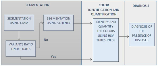
Figure 1.
Diagram describing the general strategy.
A GMM method is used in the first place because it is faster and has better segmentation in the case of images with low noise; if a high-noise background is detected, a subsequent segmentation using the PS method is performed, as that method is more robust.
For this methodology, we analyzed a total of 4977 images; a special set of 23 images, which were selected because of the challenging background, complement the 4954 images of the public dataset PlantVillage, which is used to compare the performance of the proposal to a benchmark. The analysis of the 23 images has the purpose of evaluating the performance when subject to challenging backgrounds, and the analysis of the PlantViallage dataset has the purpose of comparing the effectiveness of the proposal against previous works.
3.1. Segmentation Using GMM
In order to achieve the segmentation of the plant from the background, the intensity level of each pixel is used, that is the scale of grays; for the case of backgrounds that are solid or with low noise, the process is the following.
- Prepare the image using Gaussian Blur.
- Classify the pixels in two segments using a GMM model.
- Identify the segment that belongs to the plant.
- Closure of the segment that belongs to the plant.
3.1.1. Prepare the Image Using Gaussian Blur
Gaussian Blur is applied to the image in order to incorporate information of the surrounding pixels into each of the pixels of an image.
3.1.2. Classify the Pixels in Two Segments Using a GMM Model
A GMM model is used to separate the plant from the background, and the model is the following.
where and are the weight, mean, and variance, respectively, for the distribution that represents the plant, and are the weight, mean, and variance respectively for the distribution that represents the background.
In order to find the optimal value of the parameters of the model, given n pixels , the log likelihood function is used; in order to be maximized with the objective of finding the value of the parameters that best fit into the data, the log likelihood function is the following
The Expectation Maximization (EM) algorithm is used to find the optimal (local) values of the parameters.
- Expectation StepIn this step, the weights that the distributions belonging to the plant or the background have for each of the observations , is a latent binary variable that takes the value of 1 when it is understood that is the result of sampling from the distribution that belongs to the plant, with a probability or weight , and the same applies to the background.where is the weight that the (p) distribution of the plant has for the n observation, and is the weight that the (b) distribution of the background has for the n observation.
- Maximization StepThe means are calculatedNew variances are calculated.The values of the weights of each distribution are updated.where,
- Log likelihood evaluationWith the new parameters, the log likelihood function is evaluated, and the Expectation and Maximization steps are repeated until reaching convergence or a stop criteria.
3.1.3. Identify the Segment That Belongs to the Plant
Given the fact that a plant is a continuous entity, samples of pixels in both segments are obtained, and an average distance is obtained for both samples; the sample with the lower average distance is determined to be the one that represents the plant.
3.1.4. Closure of the Segment That Belongs to the Plant
Closure operation, a mathematical morphology operation of image analysis, is applied in order to close small gaps.
Figure 2 is presented in order to visualize the evolution of the segmentation process using GMM.
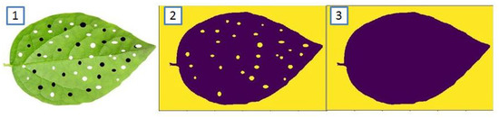
Figure 2.
Evolution of the segmentation process: (1) Original Image, (2) Segmentation obtained by GMM, (3) Segmentation obtained after closure.
3.2. Variance Ratio Evaluation
In order to evaluate if an image has a low or high-noise background, the variance of the pixels that belong to the segment associated with the background is divided over the variance of the pixels of the complete image. The variance ratio evaluation incorporates the assumption that a low-noise background is going to have a very small variance compared to the variance of the complete image; a threshold of 0.016 is selected because it optimally classifies the initial set of 23 images considered in this work and was later used in a subsequent set of 4954 images.
where,
- = Variance ratio;
- = Variance of the background;
- = Variance of the complete image.
3.3. Segmentation with Probabilistic Saliency
In the image analysis context, a salient region of the image is the part of the image that clearly stands out from the rest, and probabilistic saliency is a technique that aids in detecting the part of an image that is salient. It is expected that even when analyzing images with backgrounds with large noise, the salient object will be the plant; therefore, the following process is presented.
- Codify the image with the HSV thresholds.
- Obtain the saliency map.
- Segment the saliency map with Otsu’s method.
- Apply opening and closure operations to the segmented image.
3.3.1. Codify the Image with the HSV Thresholds
With the objective of reducing or homogenizing the background noise of the image and to increase the accuracy of the segmentation and reduce computational operations, the image is codified passing from an RGB image to a binary codification in which 1 is for the pixels that a priori may be part of the plant and 0 is for the pixel that are might not be part of the plant, and the codification criteria is the following. In this case, we expect that the black and brown colors of a plant are going to appear as holes that will be closed in the final step of the proposed process.
- White—0.
- Black—0/1 (Depending on the case).
- Green—1.
- Yellow—1
- Brown—0/1 (Depending on the case).
- Unidentified color—0 (Noise).
3.3.2. Obtain the Saliency Map
A saliency map is a representation in which to any pixel of an image that has a probability that the pixel is salient assigned, the pixels with high probabilities could be considered salient while the ones with low values may not be considered. In order to begin, a probability of 0.15 is assigned to all of the pixels.
In order to update those values, a group of windows are used to compare the salient and non-salient regions, arranged in a 15-saliency windows grid that is centered in the average x coordinate and y coordinate of all of the pixels that were considered a priori salient as a result of the codification with the neural net; this step is crucial in the reduction of processing time as we are incorporating the assumption that the place with the higher concentration of a priori salient pixels may contain the overall salient object. The dimension of each side of the grid is of the largest side of the image, and the separation between the center of a window and the next one is of the largest side of the image.
As mentioned earlier, a saliency window is used to contrast the value that a pixel has related to the rest of the pixels inside of the saliency windows vs. the values outside of the saliency window; in this research, we consider local and global saliency. Figure 3 and Figure 4 offer a visual representation of the mentioned concepts.
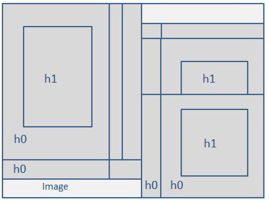
Figure 3.
Grid of saliency windows.
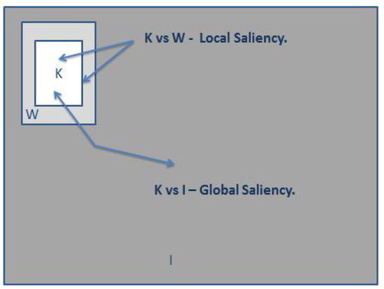
Figure 4.
Illustration of local and global saliency.
K is considered to be the salient region, W is considered to be the non-salient local region of the window, and I is considered to be the non-salient global region.
The model is the following.
- The pixel is not considered salient; it is associated with I and W,
- The pixel is considered salient; it is associated with K.
Therefore, for the case of local saliency, the salient probability is calculated as follows.
where
- is the a priori probability that the pixel is not salient;
- is the a priori probability that the pixel is salient;
- is the probability to observe the specific value of the pixel given that it is not salient;
- is the probability of observing the value of the pixel given that it is salient.
The conditional probabilities are expressed and calculated in the following way.
where
- is the number of pixels with codification 1 in W;
- is the total number of pixels in W;
- is the total number of pixels with the codification 1 in K;
- is the total number of pixels in K.
For the case of the global saliency, the process is the similar, but for the calculation of the conditional probabilities, the region I is taken into account.
Therefore, the updated saliency value after a specific window is the following.
The process is repeated for the total of 15 saliency windows that are part of the grid, and it is important to overlap the saliency windows, so the values of a specific pixel are updated several times.
It is important to state that only the pixels that were codified with “1” by the the HSV thresholds are updated. The idea is to take those a priori pixels that may be part of the segment that represents the plant and to discard those that do not belong to the salient object. By doing so, the computational efforts are vastly reduced, as all the pixels codified with a “0” are not considered and will not likely be part of the salient object.
3.3.3. Segment the Saliency Map with Otsu’s Method
Otsu’s method, a popular method for the binarization of images, is applied in order to segment the saliency map and generate a binarized image by calculating the threshold value for the saliency probabilities.
3.3.4. Apply Opening and Closure Operations to the Segmented Image
Opening and closure operations, two important mathematical morphology operations of image analysis are applied in order to close small gaps and to erase dots in the background.
Figure 5 and Figure 6 are presented in order to visualize the evolution of the segmentation process using probabilistic saliency.
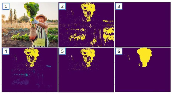
Figure 5.
Evolution of the segmentation process: (1) Original image, (2) First guess codified by HSV thresholds, (3) Initial saliency map, (4) Final saliency map, (5) Segmentation after Otsu’s method, (6) Final segmentation after opening and closure.
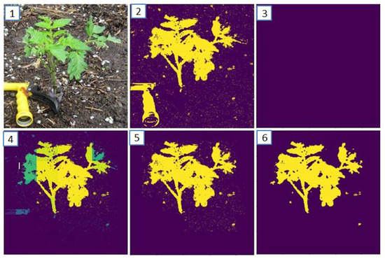
Figure 6.
Evolution of the segmentation process: (1) Original image, (2) First guess codified by HSV thresholds, (3) Initial saliency map, (4) Final saliency map, (5) Segmentation after Otsu’s method, (6) Final segmentation after opening and closure.
3.4. Color Identification and Quantification
3.4.1. Identification of Colors Using HSV Thresholds
HSV thresholds were established for the identification of white, black, green, yellow, and brown colors. Those colors were considered because they are strongly associated with plant diseases and the vast majority of plants are green; when a color that does not satisfy any of the threshold criteria, it is classified as “unidentified”.
3.4.2. Color Quantification
Once the segment belonging to the plant has been identified, the quantification of the pixels that have colors associated to the diseases is executed using the following criteria.
- White portion
- Black portion
- Green portion
- Yellow portion
- Brown portion:
where
- is the number of white pixels;
- is the number of black pixels;
- is the number of green pixels;
- is the number of yellow pixels;
- is the number of brown pixels;
- is the total number of pixels of the segment that represents the plant.
With the portions calculated now, it is possible to estimate the portion of the tissue of the plant that has the presence of the following diseases.
- White spots: White.
- Necrosis: Black portion + Brown portion.
- Healthy: Green portion.
- Chlorosis: Yellow portion.
3.5. Plantvillage Dataset and Benchmarking
In order to compare the performance of our method, we used a set of 4954 images selected from the PlantVillage dataset analyzed in [1], which employed a deep learning approach specifically trained on the dataset, which is considered the benchmark.
This dataset is composed of images of 256 × 256 dimension that belong to different classes, which are labeled as either healthy or as having only one specific disease; therefore, those images that belong to a class associated with a disease presenting colors similar to any of the three diseases considered in this work were selected.
As the proposed methods generate a diagnosis of the portion of the plant that has a specific disease, different levels of thresholds were used to transform the original portion diagnosis into a binary diagnosis. If the portion of the plant that has colors associated with a specific disease is larger or equal to a threshold, the plant is classified as having that disease.
Since the dataset is composed of classes of both healthy and diseased plants, we propose two metrics to evaluate the accuracy of the diagnosis.
- Diseased class. In the case of having a class associated to a disease, the accuracy is calculated as follows,whereACCD is the accuracy;DI is the umber of images classified as diseased;TI is the total number of images belonging to that class.
- Healthy class. In the case of having a class associated with healthy plants, the accuracy is calculated as follows,where,ACCH is accuracy,DI is number of images classified as diseased,TI is the total number of images belonging to that class.
Table 1 presents the results achieved with different levels of thresholds; the following is necessary to be specified.

Table 1.
Evaluation of some results for the PlantVillage dataset and comparison with benchmark.
- Class is the name of the class.
- SZ is the number of images belonging to that class.
- T is the average processing time in milliseconds recorded using a machine with Intel i7 @ 1.90 GHz 2.40 GHz and 8 GB RAM.
- When using a threshold of , the accuracy achieved is . If the portion of the plant that has colors associated to a disease is larger or equal to , the plant is considered diseased.
- When using a threshold of , the accuracy achieved is . If the portion of the plant that has colors associated to a disease is larger or equal to , the plant is considered diseased.
- When using a threshold of , the accuracy achieved is . If the portion of the plant that has colors associated to a disease is larger or equal to , the plant is considered diseased.
- When using a threshold of , the accuracy achieved is . If the portion of the plant that has colors associated to a disease is larger or equal to , the plant is considered diseased.
- MAX is the maximum accuracy achieved per class.
- BM is the accuracy achieved by the benchmark.
4. Results
Some of the test images and the results generated by the methods are presented in Figure 7, Figure 8 and Figure 9 in order to visually appreciate the results.
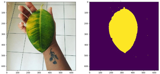
Figure 7.
White spots: , Necrosis: , Chlorosis: , Healthy: .
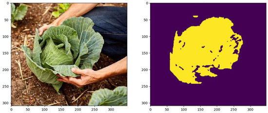
Figure 8.
White spots: , Necrosis: , Chlorosis: , Healthy: .
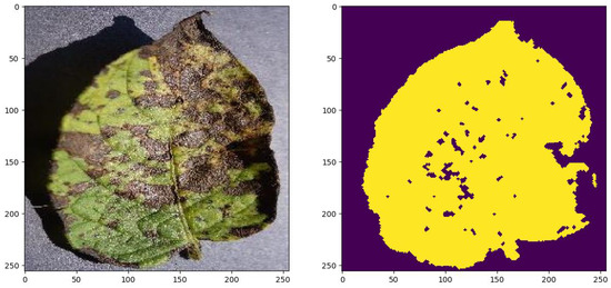
Figure 9.
White spots: , Necrosis: , Chlorosis: , Healthy: .
5. Discussion
The processing times are very competitive with all of the test images processed under 160,000 ms and an average of 22,000 ms for the special set and 5600 ms for the subsequent set. From the results obtained, it can be seen that the GMM method is more efficient on images with a controlled background, while the PS method is more efficient on images with high background noise. Future work could consider using a neural network to perform this classification of low/high noise background instead of using the variance ratio evaluation.
The results belonging to the evaluation of the performance in a generalized scenario using the PlantVillage dataset are very interesting. Considering the best accuracy per class, an overall accuracy of is achieved compared to the overall accuracy of of the benchmark, which was specifically trained for this dataset [1].
6. Conclusions
A simple proposal for the problem generating a robust diagnosis of the presence of chlorosis, necrosis, and white spots was presented; in order to do so, the task was divided in the segmentation of the plant and subsequent quantification of colors.
Compared to the benchmark, our proposal was able to outperform in 10 classes, which was an indicator of sustained performance in an untrained scenario, as intended. The benchmark [1] was selected because it provided easy and open access to the database used and the codes, and it offered an outstanding overall performance of . In addition, it was recently published in 2021, therefore representing the state of the art for this subject of study.
It is relevant to highlight that simple and generalizable assumptions were incorporated in the segmentation process for the cases of segmentation using GMM and PS models; those assumptions mostly function as a way to encode prior beliefs to the model, such as the expected colors to be present in the vast majority of plants (green) and the colors associated with the diseases. It is important to note that even though the ability to correctly produce a segmentation in several backgrounds with different types of plants was clearly achieved, at least judging by the test images included in this paper, there are cases in which those assumptions may have to be modified in order to incorporate the best fitting a priori information or beliefs into the models. In addition, the incorporation of assumptions reduced the number of computations, therefore reducing processing time, so in essence, the work presented in this paper serves as a clear statement of the power that a priori information has in order to achieve good results for a task in which that type of information is available.
Author Contributions
Conceptualization, L.G. and C.P.; Methodology, L.G. and C.P.; Software, O.M.; Data Curation, O.M.; Validation O.M.; Writing—Original Draft Preparation, L.G., C.P. and O.M.; Writing—Review and Editing, L.G., C.P. and O.M. All authors have read and agreed to the published version of the manuscript.
Funding
This research received no external funding.
Data Availability Statement
Acknowledgments
Special thanks to CIMAT Aguascalientes and the Artificial Vision Laboratory CIO Aguascalientes for their support in the generation of this work, allowing the contributors to work in their facilities.
Conflicts of Interest
The authors declare no conflict of interest.
References
- Ahmed, A.A.; Reddy, G.H. A mobile-based system for detecting plant leaf diseases using deep learning. AgriEngineering 2021, 3, 478–493. [Google Scholar] [CrossRef]
- Ferentinos, K.P. Deep learning models for plant disease detection and diagnosis. Comput. Electron. Agric. 2018, 145, 311–318. [Google Scholar] [CrossRef]
- Carranza-Rojas, J.; Goeau, H.; Bonnet, P.; Mata-Montero, E.; Joly, A. Going deeper in the automated identification of Herbarium specimens. BMC Evol. Biol. 2017, 17, 1–14. [Google Scholar] [CrossRef] [PubMed] [Green Version]
- Yang, X.; Guo, T. Machine learning in plant disease research. Eur. J. Biomed. Res. 2017, 31, 1. [Google Scholar] [CrossRef] [Green Version]
- Lee, S.H.; Chan, C.S.; Wilkin, P.; Remagnino, P. Deep-plant: Plant identification with convolutional neural networks. In Proceedings of the 2015 IEEE International Conference on Image Processing (ICIP), Quebec City, QC, Canada, 27–30 September 2015; pp. 452–456. [Google Scholar]
- Grinblat, G.L.; Uzal, L.C.; Larese, M.G.; Granitto, P.M. Deep learning for plant identification using vein morphological patterns. Comput. Electron. Agric. 2016, 127, 418–424. [Google Scholar] [CrossRef] [Green Version]
- Mohanty, S.P.; Hughes, D.P.; Salathé, M. Using deep learning for image-based plant disease detection. Front. Plant Sci. 2016, 7, 1419. [Google Scholar] [CrossRef] [PubMed] [Green Version]
- Sladojevic, S.; Arsenovic, M.; Anderla, A.; Culibrk, D.; Stefanovic, D. Deep Neural Networks Based Recognition of Plant Diseases by Leaf Image Classification. Comput. Intell. Neurosci. 2016, 2016, 3289801. [Google Scholar] [CrossRef] [PubMed] [Green Version]
- Fuentes, A.; Yoon, S.; Kim, S.C.; Park, D.S. A robust deep-learning-based detector for real-time tomato plant diseases and pests recognition. Sensors 2017, 17, 2022. [Google Scholar] [CrossRef] [Green Version]
- Petrellis, N. A smart phone image processing application for plant disease diagnosis. In Proceedings of the 2017 6th International Conference on Modern Circuits and Systems Technologies (MOCAST), Thessaloniki, Greece, 4–6 May 2017; pp. 1–4. [Google Scholar]
- Figueiredo, M.A. Bayesian image segmentation using Gaussian field priors. In Proceedings of the International Workshop on Energy Minimization Methods in Computer Vision and Pattern Recognition, St. Augustine, FL, USA, 9–11 November 2005; pp. 74–89. [Google Scholar]
- Singh, C.; Kaur, K.P. A fast and efficient image retrieval system based on color and texture features. J. Vis. Commun. Image Represent. 2016, 41, 225–238. [Google Scholar] [CrossRef]
- Luan, S.; Chen, C.; Zhang, B.; Han, J.; Liu, J. Gabor convolutional networks. IEEE Trans. Image Process. 2018, 27, 4357–4366. [Google Scholar] [CrossRef] [Green Version]
- Jiang, S.; Luo, J.; Ruiz-Pava, G.; Hu, J.; Magee, C.L. Deriving design feature vectors for patent images using convolutional neural networks. J. Mech. Des. 2021, 143, 061405. [Google Scholar] [CrossRef]
- Dong, X.; Meng, Z.; Wang, Y.; Zhang, Y.; Sun, H.; Wang, Q. Monitoring Spatiotemporal Changes of Impervious Surfaces in Beijing City Using Random Forest Algorithm and Textural Features. Remote Sens. 2021, 13, 153. [Google Scholar] [CrossRef]
- Eslami, D.; Di Angelo, L.; Di Stefano, P.; Guardiani, E. A Semi-Automatic Reconstruction of Archaeological Pottery Fragments from 2D Images Using Wavelet Transformation. Heritage 2021, 4, 76–90. [Google Scholar] [CrossRef]
- Wang, Z.; Badiu, M.A.; Coon, J.P. A Framework for Characterising the Value of Information in Hidden Markov Models. arXiv 2021, arXiv:2102.08841. [Google Scholar]
- Nemati, R.J.; Riaz, F.; Hassan, A.; Abbas, M.; Rehman, S.; Hussain, F.; Rubab, S.; Azad, M.A. A Framework for Classification of Gabor Based Frequency Selective Bone Radiographs Using CNN. Arab. J. Sci. Eng. 2021, 46, 4141–4152. [Google Scholar] [CrossRef]
- Paredes-Orta, C.A.; Mendiola-Santibañez, J.D.; Alvarado-Robles, G.; Terol-Villalobos, I.R. Ultimate opening: Invariants, anamorphoses, and filtering. J. Electron. Imaging 2018, 27, 063015. [Google Scholar] [CrossRef]
- Rocha Neto, J.F.; Felzenszwalb, P.; Vazquez, M. Direct Estimation of Appearance Models for Segmentation. arXiv 2021, arXiv:2102.11121. [Google Scholar] [CrossRef]
- Ahmadi, R.; Ekbatanifard, G.; Bayat, P. A Modified Grey Wolf Optimizer Based Data Clustering Algorithm. Appl. Artif. Intell. 2021, 35, 63–79. [Google Scholar] [CrossRef]
- Santos, J.F.B.; Junior, J.D.D.; Backes, A.R.; Escarpinati, M.C. Segmentation of Agricultural Images using Vegetation Indices. In Proceedings of the VISIGRAPP (4: VISAPP), Online Streaming, 8–10 February 2021; pp. 506–511. [Google Scholar]
- Heikkila, M.; Pietikainen, M. A texture-based method for modeling the background and detecting moving objects. IEEE Trans. Pattern Anal. Mach. Intell. 2006, 28, 657–662. [Google Scholar] [CrossRef] [Green Version]
- Sheikh, Y.; Shah, M. Bayesian modeling of dynamic scenes for object detection. IEEE Trans. Pattern Anal. Mach. Intell. 2005, 27, 1778–1792. [Google Scholar] [CrossRef] [Green Version]
- Xiang, P.; Song, J.; Qin, H.; Tan, W.; Li, H.; Zhou, H. Visual Attention and Background Subtraction with Adaptive Weight for Hyperspectral Anomaly Detection. IEEE J. Sel. Top. Appl. Earth Obs. Remote Sens. 2021, 14, 2270–2283. [Google Scholar] [CrossRef]
- Jadhav, D.A.; Sharma, Y.; Arora, P.S. Adaptive Background Subtraction Models for Shot Detection. In Advances in Signal and Data Processing; Springer: Berlin/Heidelberg, Germany, 2021; pp. 249–258. [Google Scholar]
- Montero, V.J.; Jung, W.Y.; Jeong, Y.J. Fast background subtraction with adaptive block learning using expectation value suitable for real-time moving object detection. J. Real-Time Image Process. 2021, 18, 967–981. [Google Scholar] [CrossRef]
- Mo, S.; Deng, X.; Wang, S.; Jiang, D.; Zhu, Z. Moving object detection algorithm based on improved visual background extractor. Acta Opt. Sin. 2016, 36, 0615001. [Google Scholar]
- Zhang, T.; Kang, H. An Algorithm for Motion Estimation Based on the Interframe Difference Detection Function Model. Complexity 2021, 2021, 6638792. [Google Scholar] [CrossRef]
- Chen, Y.; Hu, W. A Video-Based Method with Strong-Robustness for Vehicle Detection and Classification Based on Static Appearance Features and Motion Features. IEEE Access 2021, 9, 13083–13098. [Google Scholar] [CrossRef]
- Ghasemi, M.; Varshosaz, M.; Pirasteh, S.; Shamsipour, G. Optimizing Sector Ring Histogram of Oriented Gradients for human injured detection from drone images. Geomat. Nat. Hazards Risk 2021, 12, 581–604. [Google Scholar] [CrossRef]
- Ye, C.; Slavakis, K.; Nakuci, J.; Muldoon, S.F.; Medaglia, J. Online Classification of Dynamic Multilayer-Network Time Series in Riemannian Manifolds. In Proceedings of the ICASSP 2021–2021 IEEE International Conference on Acoustics, Speech and Signal Processing (ICASSP), Toronto, ON, Canada, 6–11 June 2021; pp. 3815–3819. [Google Scholar]
- Tortorici, C.; Berretti, S.; Obeid, A.; Werghi, N. Convolution operations for relief-pattern retrieval, segmentation and classification on mesh manifolds. Pattern Recognit. Lett. 2021, 142, 32–38. [Google Scholar] [CrossRef]
- Singh, V.K.; Kumar, N. SOFT: Salient object detection based on feature combination using teaching-learning-based optimization. Signal Image Video Process. 2021, 15, 1777–1784. [Google Scholar] [CrossRef]
- Kousik, N.; Natarajan, Y.; Raja, R.A.; Kallam, S.; Patan, R.; Gandomi, A.H. Improved salient object detection using hybrid Convolution Recurrent Neural Network. Expert Syst. Appl. 2021, 166, 114064. [Google Scholar] [CrossRef]
- Wang, H.; Zhu, C.; Shen, J.; Zhang, Z.; Shi, X. Salient object detection by robust foreground and background seed selection. Comput. Electr. Eng. 2021, 90, 106993. [Google Scholar] [CrossRef]
- Jian, M.; Wang, J.; Yu, H.; Wang, G.; Meng, X.; Yang, L.; Dong, J.; Yin, Y. Visual saliency detection by integrating spatial position prior of object with background cues. Expert Syst. Appl. 2021, 168, 114219. [Google Scholar] [CrossRef]
- Guo, C.; Ma, Q.; Zhang, L. Spatio-temporal saliency detection using phase spectrum of quaternion fourier transform. In Proceedings of the 2008 IEEE Conference on Computer Vision and Pattern Recognition, Anchorage, AK, USA, 23–28 June 2008; pp. 1–8. [Google Scholar]
Publisher’s Note: MDPI stays neutral with regard to jurisdictional claims in published maps and institutional affiliations. |
© 2022 by the authors. Licensee MDPI, Basel, Switzerland. This article is an open access article distributed under the terms and conditions of the Creative Commons Attribution (CC BY) license (https://creativecommons.org/licenses/by/4.0/).