Abstract
Virtual reality (VR) is increasingly important for exploring the real world, which has partially moved to virtual workplaces. In order to create immersive presence in a simulated scene for humans, VR needs to reproduce spatial audio that describes three-dimensional acoustic characteristics in the counterpart physical environment. When the user moves, this reproduction should be dynamically updated, which provides practical challenges because the bandwidth for continuously transmitting audio and video scene data may be limited. This paper proposes an interpolation approach for dynamic spatial audio reproduction using acoustic characteristics of direction and reverberation at limited numbers of positions, which are represented using a first order Ambisonics encoding of the room impulse response (RIR), called the directional RIR (DRIR). We decompose two known DRIRs into reflection components, before interpolating early dominant components for DRIR synthesis and utilizing DRIR recordings for accuracy evaluation. Results indicate that the most accurate interpolation is obtained by the proposed method over two comparative approaches, particularly in a simulated small room where most direction of arrival estimation errors of early components are below five degrees. These findings suggest precise interpolated DRIRs with limited data using the proposed approach, which is vital for dynamic spatial audio reproduction for VR applications.
1. Introduction
Virtual reality (VR) is one of the most fundamental efforts of humans to explore the real world using a simulated environment. With the outbreak of the unprecedented coronavirus disease (COVID-19), the world has progressively and partially changed to virtual workplaces, making VR-related technologies increasingly vital for applications, such as teleconferencing, remote teaching, telemedicine and so on. VR is only viable when creating an immersive experience for people as if they were physically present in the target real-world place. To implement this, VR sessions are required to reproduce the spatial audio that is perceived to provide the three-dimensional (3D) acoustic characteristics of the real environment, including sound source direction and reverberation. This is typically achieved using binaural reproduction techniques over headphones. As VR users are inclined to move around the virtual space, the spatial audio needs to be reproduced dynamically to match the user’s location relative to the sound source. Due to the limited storage in real-world products, the dynamic reproduction usually requires continuously transmitting binaural signals through telecommunication to match the user position, which provides practical challenges because the transmission bandwidth can also be limited. Thus, an efficient and effective method is urgently needed for dynamic spatial audio reproduction.
Rather than continuously transmitting binaural signals, current approaches reproduce the binaural signals at the user using knowledge of the sound source, the user’s head related transfer function (HRTF) and the room impulse response (RIR), both of which describe the acoustic transfer function between a sound source and a receiver, depending on their relative position and depending also on the unique characteristics of the listener for HRTF. In this paper, we assume the sound source is known (e.g., through transmission of dry audio source signals at the start of a VR session) and the HRTF is accurately known for a user. To reproduce the spatial audio, the RIR needs to be convolved with the sound source for all possible positions that the user can walk through, so all RIRs at such positions need to be known. This still presents practical challenges in bandlimited environments. Therefore, this paper focuses on using interpolation approaches that can estimate RIRs at unknown positions using a limited set of known RIRs.
A conventional RIR is measured either by recording an impulse signal [1] or synthesized using approaches, such as the well-known image method [2], but these are one-dimensional signals in the time domain and do not contain spatial information, such as the direction of arrival of the source. Hence, researchers have investigated approaches to interpolating RIRs using 3D representations of the RIR, such as first order Ambisonics (FOA) encodings, which are known here as directional RIRs (DRIRs). Mariette and Katz [3] utilized a virtual FOA microphone array to achieve a simple implementation, which calculated the weighted average of recorded B-format signals to estimate unknown DRIRs with the weights decided by distances from the source to each microphone. Southern et al. also applied a similar linear approach to real-time acoustic space auralizations [4]. These algorithms require no assumptions or priori knowledge and are straightforward to use, whereas their interpolation accuracy is limited due to the spectral distortion and large localization errors occurring particularly when the sound source is close to both microphones or closer to one microphone than to another [5]. Typical solutions to address this limitation utilize higher order Ambisonics (HOA) representations of the soundfield, which provide improved accuracy over a larger spatial region. Approaches based on HOA representations include extrapolation-based algorithms [6,7,8,9,10], which extrapolate a finite set of spatial parameters based on measured RIRs and thus allow the RIR to be synthesized outside the region covered by microphones. While such extrapolation approaches can introduce inaccurate source localization and audible processing artifacts, such as spectral coloration [11], a number of interpolation-based approaches using HOA microphone array recordings are prone to mitigate these effects, such as the regularized least-squares interpolation approaches using spherical harmonic translation coefficients [12,13,14,15]. More recent related work [16,17] utilized frequency-dependent regularization to limit spectral variation and exclude any microphones closer to a sound source than to the target listening position in order to obtain accurate results for near-field sources. While promising, HOA representations require many more channels compared to FOA representations, which may not be desirable in low bandwidth applications.
Hence, this paper focuses on FOA representations for improving the accuracy of interpolation and localization in limited bandwidth scenarios, which considers parametric approaches to interpolate known DRIR signals to reproduce the DRIR at a new position. The approach is inspired from earlier research that identifies, localizes, and isolates discrete sound sources in the time-frequency domain before treating them as virtual sound sources to achieve soundfield navigation [18,19]. While the previous work separated anechoic FOA recordings of sound mixtures into multiple virtual sources, this paper centers on separating FOA DRIR recordings into virtual components representing the directional and reverberant components, focusing on the early specular reflections. The approach assumes the DRIR is recorded or represented as an FOA (B-format) encoding at a finite number of known positions within a virtual environment, for example covering a grid of locations across the room. Based on knowledge of the user position, the known DRIR signals at the two closest positions in the grid are decomposed into the FOA representations of the direct sound, specular reflection, and diffuse signals. The specular reflection FOA signals are analyzed in the time domain to estimate individual specular reflections and their corresponding directions of arrival (DOAs) and time of arrival (TOA); these components are then formed into FOA signals representing virtual image sources. At the new listening position, direct sound and early specular reflections are estimated using the corresponding DOA and TOA of these virtual sources and a known FOA signal. The motivation of using the DOA and TOA information of early specular reflections is that sounds arriving up to 50 ms are inclined to be perceived as mixed together instead of as individual echoes. Their timing and directions impact spatial perception significantly on the depth and broadening of sources, as well as the size of the space and the distance to surfaces [20]. In addition, including the DOA of the early reflections allows their direction to be adjusted as the listener turns their head during a VR session. Hence this information can enable increased immersive perception, as if users are in the real target environment. The approach is compared with two representative navigational methods based on FOA representations [4,16] and working on guaranteeing the high accuracy in estimating the DOA and TOA of the direct sound and estimated early specular reflections.
The remainder of this paper is organized as follows. Section 2 analyzes the signal model and decomposition of FOA recordings, before introducing an approach to extract the DOA information and interpolate DRIRs at positions where microphones are not available. Section 3 conducts experiments using both real-world and simulated DRIR recordings to validate the proposed algorithm, and Section 4 compares the experimental results with that of two previous representative approaches. Contributions and discussions are concluded in Section 5.
2. DRIR Interpolation Framework
The interpolation framework assumes that the DRIR has been recorded or synthesized at multiple locations in a room. An example is shown in Figure 1a, which illustrates a grid of FOA recordings obtained within a classroom at the University of London [21] and used in this paper. Figure 1b illustrates the interpolation approach using two of the known FOAs. This section describes the signal model and approach used to decompose the DRIR into estimated direct sound and specular reflection components.
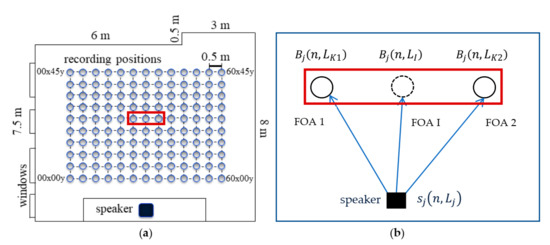
Figure 1.
FOA interpolation based on a grid of known FOAs for a single source where j = 1: (a) locations of known FOAs; (b) example FOA interpolation using every second known FOAs (FOA 1 and FOA 2) to find the interpolated FOA (FOA I). Red rectangles indicate chosen grid points.
2.1. Overview of the Interpolation Approach
The FOA at location (assuming a 3D acoustics model) at discrete time and in a noise-free environment is assumed to be:
where is the jth (j = 1, 2, …, J) source originating at location , is the corresponding RIR between the source at location and recording location , and is the convolution operator. For recording the RIR signal as A-format using four microphones in the standard tetrahedral arrangement [22] surrounding the central location , we assume the RIR for source j at each of the four channels are given by , , , and (labeled as , , , and for short in the following descriptions), where the relative locations of each microphone can be found by standard equations for B-format. The resulting B-format channel signals converted from the A-format recordings are represented as [22]:
In a compact form, the FOA signals can be represented as:
Figure 1 illustrates the DRIR interpolation approach for a single source (j = 1) when using two FOA recordings at locations and to find the interpolated FOA signal at location . The proposed method can be summarized as follows:
- Separate the FOA signals of DRIR into the direct sound, the specular reflection signals and the chaotic diffuse components;
- Analyze the W channel of the separated direct sound and specular reflection FOA signals to locate peaks corresponding to estimated image sources;
- Form a new FOA signal for this image source using a segment of the signal surrounding this peak for the W channel and corresponding X, Y, and Z channels;
- Repeat until a desired number of image sources (peaks) have been extracted;
- Interpolate such FOA signals and their extracted DOA information at two closest recording positions to the listening position using a weighted average approach;
- Synthesize the FOA signal of DRIR at the listening position utilizing the interpolated parameters and a known FOA signal recorded closely.
2.2. Separating FOA Signals into Specular and Diffuse Components
The approach we propose here is based on analyzing the FOA signals to find short segments of signals containing local peaks that are compared against energy thresholds. This is inspired by approaches to tracking noise levels in audio signal processing and, in particular, the approach of [23], which aims to distinguish between short-duration impulsive noise and longer duration increases in the noise level. Here, this approach is used to separate the DRIR into the direct sound, specular components (similar to impulsive noise components, including the direct sound) and diffuse components (similar to noise signals) through the comparison of the output power from two tracking filters: a fast and a slow tracker filter applied to shorter and longer duration segments, respectively. For each FOA impulse response in this paper, a RIR cleaner is firstly applied to remove the direct current components (achieved by designing a high pass filter with cut-off frequency set to 20 Hz, corresponding to the minimum audible frequency by the human listening system). The four-channel FOA DRIR is then normalized with any silence parts removed.
The cleaned FOA DRIR is then decomposed into the direct sound, several specular components and diffuse components. This is achieved by analyzing the power of the W channel with a fast and a slow tracker as follows:
where is the power of the W channel of the DRIR signal, is the convolution operator, and and are filters that derive the average short-term and longer-term power within the region centered at time n, respectively. These signals will be analyzed to find short-term peaks in the average RIR power relative to the longer-term average RIR power and as explained further below. Note that this approach is most suited to the direct sound and early specular reflections where it is assumed that these are adequately separated in time. Later sections of the DRIR, where individual components are located closer in time and not extracted by the specular analysis approach, are assumed diffuse and would be synthesized using existing decorrelation techniques [24] or a decaying noise model rather than interpolation. These filters are based on window functions, and are defined as follows:
where and are Hanning windows centered at sample time n, with their lengths corresponding to the chosen discrete time constants of and , respectively. Both and denote the continuous time lengths selected for the two weighted average filters in (6) and (7), separately, with being the sampling frequency of the DRIR recording. By looking into the ratio of the resultant filtered power to from (4) and (5), the salience of their difference can be measured for peak detection, which is highly related to the ratio of to . In this paper, 0.0003 (s) and 0.002 (s) were chosen based on informal experiments, which generally mean fine-tuning parameters for finding the optimal around a measured or empirical value of parameters that are not well-determined for a practical application. Similar experiments have been conducted for two other thresholds in this section. For the ratio of to , there is an empirical value of 0.1 for peak detection applications, and the magnitude of a few milliseconds of matches the time length of specular reflections considering the employed dataset [21] in this paper. Thus, based on the two conditions, a series of tests on different values indicate that the elected and present the most salient power difference between and , which is used to find the direct sound and specular reflections:
where the peak of the ith specular reflection (with the 1st peak being the direct sound) is detected at time when the followings are met:
- is greater than a pre-defined threshold (in this work = 4 dB was chosen, under which ). Informal experiments found that should be in the range from 4 dB to 6 dB to avoid sensitivity of the approach to this threshold. For an smaller than 4 dB, this can lead to a few false peaks being extracted and if is greater than 6 dB it can lead to some clear peaks not being detected. This was initially verified by analyzing results from a sub-set of DRIR recordings, whilst the TOA results in Section 4 analyze this more thoroughly.
- is a local maximum.
- is greater than a pre-defined threshold , which distinguishes the peak from background noise, so the selection of depends on the noise floor level of specific DRIR recordings (in this work = −50 dB was chosen to match the noise floor of the chosen recordings [21], but in practice this could be adjusted to match the estimated noise floor level for recordings in another room).
Considering the W channel as an example, the ith specular reflection signal for source j recorded at location , , can be extracted from the samples of corresponding to where is larger than around each position of the specular reflection peaks. Note that decides the length of specific specular reflections in the time domain and, according to our informal experiments, a range of from 3 dB to 4 dB was found to maintain good decomposition of specular reflections. If is outside this range, it may lead to combining two specular reflections into a single component. We found that an of 4 dB, chosen for peak detection in (8), leads to specular reflections of around 0.002 s duration. For convenience, we utilize a time constant of 0.002 s for the resultant specular reflections. Thus, is found as
where , . is the time corresponding to the detected peak of the ith specular reflection , M corresponds to the chosen number of specular reflections to extract, and is a pre-defined time duration (0.002 s) that decides the length of this specular reflection in the time domain. In this way, the specular reflections are obtained as segments of DRIR recordings of the jth source. The whole diffuse signal, can be derived by removing all specular components :
where for , and for for all i. Note that if , then we assume the extracted segments would be perceived as diffuse components rather than individual specular reflections. This would require appropriate choice of the threshold based on perception, which will be considered as part of future work. Here, we focus on extracting less than 10 specular reflections, which are dominant components in DRIRs and are generally sufficiently separated in time for the DRIR databases considered.
Figure 2 shows an example of the direct sound component of the DRIR that is extracted from the FOA W channel, sampled at 48 kHz, using this approach. Shown in Figure 2a are the original RIR and the power from the fast and slow trackers, whilst in Figure 2b, the resulting direct sound is illustrated as well, which is overlaid on top of the RIR recording. Figure 3 shows an example of the early reflections extracted from the FOA W channel for the same RIR corresponding to Figure 2. To clarify the blue curve in Figure 2b, the extracted direct sound is the received copy of the RIR signal at the W channel microphone, so the orange-colored curve is overlaid on top of the blue curve, as indicated in the legend. In Figure 3b, three main orange-colored peaks are found as specular reflections, which are received later than the direct sound in Figure 2b and are also on top of the blue curve. Figure 2a and Figure 3a are plotted to make the blue curves observable.
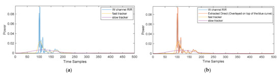
Figure 2.
Direct sound component extracted from the W channel of the FOA RIR recording. Plotted are the power of the original RIR (blue), extracted component (orange), fast tracker (yellow), and slow tracker (purple): (a) without the direct sound (orange); (b) with the direct sound that is overlaid on top of the W channel RIR recording (blue curve).
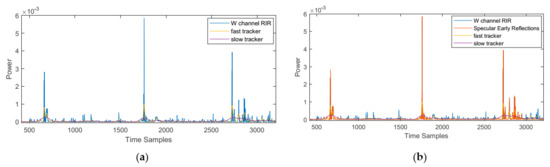
Figure 3.
Early reflections extracted from the W channel of the FOA RIR recording. Plotted are the power of the original RIR (blue), extracted reflections (orange), fast tracker (yellow), and slow tracker (purple): (a) without the specular reflections (orange); (b) with the specular reflections that are overlaid on top of the W channel RIR recording (blue curve).
Once the specular reflection signals have been extracted, these can be separated into individual specular reflections, . From each of the four channels of the FOA signal, a new FOA signal can then be formed for this image source. For a given sound source, j, the FOA signals for each corresponding specular reflection (denoted by i) are described as:
where corresponds to the specular reflection i extracted using (9) and , , and are found by extracting the samples corresponding to the same samples of the specular reflections of .
2.3. Deriving the DOA for the FOA Encoded Image Sources
Once the FOA signals at the two known locations have been decomposed into direct sound and specular reflections, these are analyzed to find the corresponding DOA of the direct sound and virtual image sources. Using this information, the DOA of the direct sound and reflections at the new location can be obtained using interpolation.
The DOA of each FOA-encoded image source is determined using an existing approach to DOA estimation from B-format recordings [18] that has been found to provide accurate results when used for finding the DOA of multiple sources. Here, this method is applied to the FOA recordings of the specular reflections. The FOA encoding of the specular reflections of (11) is first converted to the time-frequency domain using the short-term Fourier transform (STFT), resulting in (labeled as a simplified version of in (12) and (13)), where k denotes discrete frequency. Here, a 1024-long STFT with 50% overlapping Kaiser-Bessel derived windows are used. The azimuth and elevation of each time-frequency instant, (, are given by:
where the operator (Re) fetches the real part of a complex number, and the bar above a complex number () represents the conjugation operation. The time-frequency DOA estimates of (12) and (13) are calculated across the duration of the FOA signals and formed into a histogram, where the histogram bar represent the count of each DOA value and each histogram bin represents one degree resolution. Analyzing the histogram peaks provides an estimated DOA for the virtual image source (for full details, see [18]).
2.4. Deriving the Interpolated FOA Signals at the Virtual Listening Location
The framework considered in this paper assumes the two closest FOA signals recorded at positions and are used to find the interpolated FOA at an arbitrary interpolation position , with the listener looking towards the source of interest (see Figure 1). As an initial exploration, the interpolated DOA in this work is found using a linear interpolation approach that calculates the weighted average, formulated as follows:
where and are the distance from to and , separately. This method is applied to interpolate for the direct sound and specular components using corresponding extracted DOAs from the W channels of the two FOA recordings (FOA 1 and FOA 2 in Figure 1). Note that the formulations consider the scenario where the listening position is closer to one of the two known positions. The closer recording contributes more than the other in the interpolated result, so the proportion defined for and at is the distance from to , , divided by the overall distance .
Next, the TOAs corresponding to the peak of the direct sound and specular reflections are found by using linear interpolation of the TOAs of the direct sound and specular reflections found in the two known FOA recordings as:
where is the interpolated time (in samples) for one window, and and are the TOAs (in samples) of peaks in the direct sound and specular reflections extracted from the two FOA microphones, respectively. With this information, the interpolated FOA signal can be found using the two known FOA recordings along with the interpolated TOA and DOA. This is achieved by taking the direct sound and specular reflections extracted from the known FOA recordings and encoded as individual FOA signals (see Equation (11)) and creating new FOA encodings of these reflections using the interpolated DOA and standard B-format encoding functions. The process is repeated up to the desired number of image sources. The peaks of these interpolated specular reflections are shifted so that they are located at the interpolated TOA of (16); this ensures that they are correctly located in time relative to the direct sound component. The final interpolated DRIR signal is obtained by summing the direct sound and time-shifted interpolated reflections. The final interpolated FOA signal is obtained by adding the interpolated specular component to the diffuse component, which is based on the diffuse component extracted from one known FOA recording and as derived in (10).
When extracting the specular reflections from two FOA recordings, it is important that the reflections corresponding to the same image source (e.g., same first order reflection from the same wall) are used in the interpolation. If not, there is a risk that the DOAs used from both specular reflection components will correspond to different wall reflections and so result in an incorrect reflection DOA at the interpolated location. One approach to address this is to check the TOA of both specular reflections extracted from the two known FOA recordings. Provided that the known locations are not too far from each other, the amplitude of the extracted specular reflections will be similar (within a threshold), and the TOA can be used solely to identify any matching specular reflections.
To first evaluate if this was a problem in practice, an analysis was conducted for 500 interpolated DRIRs corresponding to 15 different positions in the classroom to be introduced in Section 3. This analysis compared the TOA for interpolated specular reflections with the TOA for the same specular reflection in the known (ground truth) DRIR at the same location. It was found from this analysis that there were only 10 cases (2%) where the TOA differences indicated a possible mismatch in the specular reflections. For these 10 mismatch cases, it is found that the TOA of the interpolated specular reflection is closer to the TOA of the next specular reflection in the known DRIR (e.g., the first interpolated specular reflection corresponds to the second specular reflection in the known DRIR), which is automatically corrected in the proposed algorithm. Hence, for the dataset to be experimented in Section 3, it was determined that the vast majority of early reflections extracted from the known DRIR locations were matched, and the few mismatched specular reflections in this paper have been automatically corrected.
Further research can be conducted to evaluate this issue for a wider variety of locations in the room utilizing more information of the recording environment. For example, if knowledge of the wall locations is available, it will be possible to use the estimated DOAs of two specular reflections extracted at two locations to check if they triangulate at the expected virtual image source location. It is noted that an alternative approach to interpolating the TOA for the specular reflection that takes account of differences in path length may also lead to improved accuracy and will be considered in future work.
The proposed method is highly efficient because rather than having to transmit a large set of densely located DRIRs, a smaller set of more widely spaced DRIRs can be transmitted to cover the current region where a user is located within a virtual room. Hence, rather than transmitting a new DRIR to the end device to match the new listening position, interpolation is used to find the new DRIR from the smaller set of transmitted DRIRs. To further evidence the high efficiency, it is worth analyzing the time computational complexity (TCC) of the algorithm.
- Signal decomposition: the convolution operation in (4) and (5) is implemented using an overlap-add approach based on Fast Fourier Transform, which possesses a TCC of with being the window length [25]. The weighted average filters in (6) and (7) show a TCC of , followed by the peak salience calculation in (9) and value assignments in (10) and (11), with all having a TCC of where is the length of recording.
- Deriving DOA and TOA information: (12) and (13) include STFT calculations and thus have a TCC of with being the length of the window adopted.
- Interpolating and synthesizing FOA signals: the summation in signal synthesis shows a TCC of , which is not increased by the efficient interpolation operation.
Therefore, the proposed algorithm concatenated by the three steps has an overall TCC of , which is highly efficient and suitable for end VR devices.
The efficiency of the proposed method is compared with the weighted average approach in [4] as a baseline due to their similar interpolating processes. The baseline method does not decompose signals or utilize the DOA and TOA information, which solely utilizes the third step of the proposed algorithm, leading to a TCC of . The baseline method is highly efficient, but note that the TCC of is not necessarily smaller than , as is usually much larger than the window length . Comparison results of the two TCCs depend on the specific values of and . The other comparative approach in [16] shows parametric calculation of the matrix order, singular value decomposition, regularized pseudoinverse and so on. The TCC comparison with this method is beyond the scope of this paper.
3. Experimental Setup
Experiments are designed to validate the proposed DRIR interpolation algorithm and check its performance in terms of the accuracy of the interpolated DOA and TOA. Four databases are utilized in these validations, including the real-world B-format recordings in a classroom and a great hall at the University of London [21] and simulated recordings for these two rooms using the image method [2].
3.1. Real-World DRIR Recordings
The real-world DRIR recordings were created using the sine sweep technique [26] with a Genelec 8250A loudspeaker and two microphones, an omnidirectional DPA 4006 and a B-format Soundfield SPS422B. The sampling frequency of recordings is 96 kHz.
The classroom is approximately 9 m 7.5 m 3.5 m (236 m3) in size with reflective surfaces of a linoleum floor, painted plaster walls and ceiling, and 130 positions within a central area of 6 m 6 m were selected to record the impulse response. Desks and chairs that usually fill the classroom were moved and stacked to the side against the windows when measuring. The selected positions were 50 cm apart, arranged in 10 rows and 13 columns relative to the speaker, with the seventh column directly on an axis with the speaker. This arrangement can be found in Figure 4a [21]. Note that the labels of recording positions start from “00x00y” which can be seen as the origin of the two-dimensional recording area, and the two numbers indicate the coordinates along the x axis and y axis within the position array, separately. The unit is 10 cm in the classroom, so “60x00y” means the position located at 6 m away from the origin on the x axis in the classroom.
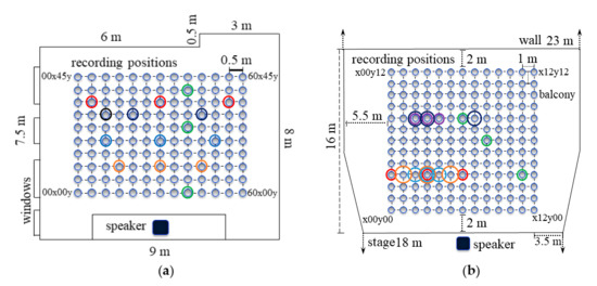
Figure 4.
In both real-world and simulation cases, illustrating the microphone positions that are selected to interpolate in: (a) the classroom horizontally at rows 3, 5, and 8 (orange, blue, and red circles), row 7 (black circles), and vertically at column 9 (green circles); (b) the great hall horizontally at row 4 (red, orange, and blue circles), row 9 (purple and black circles), and diagonally using rows 4, 7, and 9 (green circles).
For the great hall, which is approximately 23 m 16 m in size and has the capability of holding approximately 800 seats, DRIRs were recorded at 169 locations covering a central rectangular region of 12 m 12 m. The chairs were cleared when recording to avoid reflections. The great hall also contains a balcony that is 20 m beyond the rear wall. The recording locations in the great hall have a 1 m spacing in an arrangement of 13 rows and 13 columns, and the loudspeaker is on axis with the middle (seventh) column of recording positions, so “x12y00” represents the location that is 12 m away from the origin on the x axis. The great hall experimental settings can be seen in Figure 4b.
3.2. Simulated DRIR Recordings
In order to present additional comparative results with the real-world recording, the DRIRs were simulated (using the image method implemented in Matlab R2021a, named RIR Generator [27]) within two rooms of comparable size to the classroom and great hall at the same recording locations (see Figure 4).
While the room geometry is mostly the same as the classroom and great hall at the University of London [21], they are simplified to be rectangular and measuring “9 m 7.5 m 3.5 m” and “23 m 16 m 10 m”, respectively. The locations of the sources and microphones within the rooms also mimic the classroom and great hall arrangements, separately. The source is placed at (4.5, 0.5, 1.5) meters in the simulated classroom and at (11.5, 0, 1.5) meters in the simulated great hall, respectively. The origin of the microphone array “00x00y” is (1.5, 1.8, 1.5) meters in the classroom and is (5.5, 2, 1.5) meters in the great hall (the origin is assumed at the bottom left of the room). Firstly, the A-format recording is obtained four times at each of the arbitrary positions under a sampling frequency of 96 kHz, and for each of the four recordings, hypercardioid microphones pointing at specific orientations are utilized.
Another factor that needs to be considered is the reverberation time (RT) of the two rooms. Due to irregular room shapes and variable room acoustics, the RT of the real-world and simulated rooms cannot be exactly the same. In the simulated room, the RT is configured to be 1.8 s in the classroom and 2.0 s in the great hall as a constant, which are approximately the average RT of the real-world classroom and great hall, separately [21].
Finally, 130 sets of B-format recordings are obtained in both the real-world and the simulated classrooms, and 169 sets of DRIRs are recorded using B-format microphones in both the real-world and the simulated great halls. The proposed DRIR interpolation algorithm is then applied to these four databases for performance evaluation.
4. Results and Analysis
Using the databases described in Section 3, an experiment was conducted to evaluate the DRIR interpolation performance when choosing different listening positions and locations of the known DRIRs. Two representative approaches of DRIR interpolation are compared, including the linear interpolation proposed by Southern [4] and the regularized least square algorithm by Tylka [16]. Firstly, a conventional linear approach similar to the proposed method is needed as a baseline in order to compare the performance of the proposed method; the conventional linear approach chosen is the one used in [4]. The only difference between the two algorithms is the signal decomposition and synthesis process based on the DOA and TOA information of the direct sound and first few specular reflections, which is crucial for guaranteeing the listeners’ immersive perception. Secondly, a recent parametric method that shows high RIR interpolation accuracy is desired to be compared with to mainly evaluate the accuracy of the proposed method, and thus we chose [16] for this comparison. Moreover, the number of existing spatial audio reproduction approaches using B-format to record the soundfield for RIR interpolation is limited. The methodologies in [4,16] well match the proposed approach in general and are also the representative ones for comparisons in the research field. The performance was measured by finding the DOA estimation error and the TOA error for each of the extracted direct sound and specular reflections, which are dominant components of the overall FOA signal. The DOA estimation error is the absolute angular error between the azimuths and elevations derived for extracted specular reflections from the interpolated and known (ground truth) DRIRs at the chosen listening points. The TOA error is the absolute error between the time-points of the peaks of the direct sound and specular reflections extracted from the interpolated and known DRIRs at the chosen listening positions.
4.1. Comparative Analysis in the Classroom
There are five representative cases selected to compare the performance of the proposed DRIR interpolation algorithm with the previous representative methods from Southern [4] and Tylka [16] applied to the classroom databases, which are arranged as shown in Figure 4a. Although the proposed method is designed to utilize the FOA recordings closest to the listening position, it will be interesting to compare the performance in more challenging scenarios with the larger distances between known recordings and irregular spacing between the listening position and two known positions. Here, five scenarios are chosen to further highlight the advantage of the proposed approach.
4.1.1. Example Interpolated DRIR Signals
Taking row 3 as an example, the middle recording position labelled as “30x10y” is taken as the reference point, and the DRIR recording at this location is the ground truth for DRIR interpolation of the two side positions, “15x10y” and “45x10y”. The proposed algorithm firstly separates the recorded DRIR into two parts, the specular reflections (including the direct sound) and diffuse reflections. After this, the algorithm further decomposes the specular reflections into different components and obtains their corresponding image sources and DOAs. By interpolating this information for each component in the direct sound and specular reflections at the selected two side positions in each considered row, the interpolated DRIR at the listening position in that row can be obtained by combining these interpolated components with a known FOA recording. The overall interpolated DRIR in row 3 is illustrated in Figure 5, which is compared with the known (ground truth) recording at the same position, with the x-axis being the number of discrete time samples and y-axis being the normalized amplitude of the W-channel FOA recording.
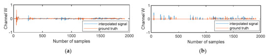
Figure 5.
Comparison plots of the W channel of the overall interpolated DRIRs using the proposed algorithm in this paper with the ground truth in row 3 considering: (a) the real-world classroom recording; (b) the simulated recording.
Taking the W channel of the interpolated DRIR as an example, it can be visually seen that generally the interpolated DRIR obtained by utilizing the proposed method accurately matches the ground truth for both databases. In the real-world classroom, the W channel almost exactly matches the ground truth, whereas the amplitude is a little lower. As for the simulation, the interpolated DRIR highly matches the ground truth due to the ideal acoustics and recording arrangements in the room, whereas the amplitude of all interpolated DRIRs is a bit larger, which may be due to extra summations of interpolated components.
4.1.2. DOA and TOA Error Results
As introduced at the beginning of Section 4, DOA and TOA errors will be analyzed for the proposed algorithm and other two comparative approaches proposed by Southern and Tylka, respectively (implemented with the code in [28]). These results for the direct sound and the first five specular reflections in the investigated cases using the real-world and the simulated databases are compared in Figure 6 and Figure 7, separately. The first group of bars in the two figures corresponds to the direct sound, and the second to sixth correspond to the first to fifth extracted specular reflections.
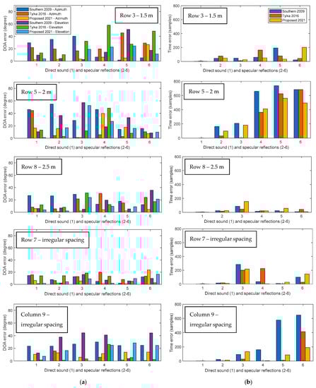
Figure 6.
Bar charts comparing the accuracy of the Southern’s method in 2009, the Tylka’s method in 2016, and the proposed DRIR interpolation algorithm in the real-world classroom arranged, as shown in Figure 4a, including: (a) the error of azimuth and elevation; (b) the error of TOA. All errors are calculated as the absolute difference between the interpolated signal and the ground truth for regular spacing cases in row 3, row 5, and row 8, as well as irregular spacing cases in row 7 and column 9, respectively (from top to bottom in each subplot).
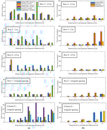
Figure 7.
Bar charts comparing the accuracy of the Southern’s method in 2009, the Tylka’s method in 2016, and the proposed DRIR interpolation algorithm in the simulated classroom arranged as shown in Figure 4a, including: (a) the error of azimuth and elevation; (b) the error of TOA. All errors are calculated as the absolute difference between the interpolated signal and the ground truth for regular spacing cases in row 3, row 5, and row 8, as well as irregular spacing cases in row 7 and column 9, respectively (from top to bottom in each subplot).
When looking at the error of the interpolated DOA, the proposed DRIR interpolation algorithm shows, generally, the smallest average errors of the azimuth and elevation in all sub-figures amongst the three approaches, which means the most accurate extractions of DOA information of the direct sound and specular reflections for synthesizing overall interpolated signals at the target listening position in both the real-world and the simulated classrooms. This advantage is particularly obvious in the simulation, where almost all errors in the first four cases using the proposed method are close to zero, with small errors of nearly five degrees appearing in column 9. The Tylka’s approach shows strength in interpolating for column 9 in the real world, presenting the smallest errors of azimuth and elevation estimation for nearly all of the direct sound and specular reflections. The Southern’s method and the Tylka’s method generally show similar errors for the azimuth and elevation in Figure 6 and Figure 7, whereas in column 9 for both databases, the Southern’s method leads to larger errors.
As for the TOA error of the direct sound and specular reflections compared with the ground truth, the two comparative methods generally present equivalent TOA errors in the real-world classroom, with the proposed DRIR interpolation method showing slightly lower TOA errors. The Southern’s method leads to slightly large errors in Figure 6b, especially for row 5 and column 9, where the errors of late reflections can reach 600 samples, i.e., 600/96,000 6.25 ms. In the simulation, Tylka’s algorithm suffers from large TOA errors at a few peaks (e.g., peaks 5 and 6 in the row 5 case of Figure 7b). Southern’s method also shows large TOA errors at a few peaks (e.g., peaks 5 and 6 in the column 9 case of Figure 7b). The proposed approach has, in general, the lowest errors, whereas it also shows a large error at peak 6 in column 9 in the case of Figure 7b.
Moreover, due to the ideal configuration of the simulated classroom, the distribution pattern across the six components for each method in all subplots of Figure 7 look similar. These results obtained in the classroom present performances of the three comparative DRIR interpolation methods in a smaller room. It can be observed that, generally, the closer the microphones are located to the sound source, the larger the DOA and TOA errors are. Note that here we have evaluated the two limited scenarios using conventional weighted-average interpolation approaches, such as the Southern’s approach, where the source is close to both known recording positions (row 3) as well as the source being closer to one recording position than to the other (row 7 and column 9). The proposed method in these cases shows reduced errors compared to the traditional linear method designed by Southern, which indicates that the limits of large localization errors mentioned in [5] is mitigated by the proposed scheme.
Additionally, an error measurement of direct-to-reverberant ratio (DRR) is introduced to describe acoustic characteristics of signals and to evaluate the accuracy of the proposed interpolation algorithm by assessing the difference between the interpolated and the known recording signals. The DRR is defined as the ratio of energy between the direct sound and all of the reverberant signals, formulated as [29], where X is the sampled signal to be evaluated, represents the occurring time (in terms of the number of samples) of the direct sound in the recording, and C is the number of samples to define the range of time of the whole direct sound signal. (C should be equivalent to 2.5 ms according to [30].) means the snippet of signal X from Sample to Sample , which is expressed in MATLAB code and so is . The DRR in this paper is implemented with the code in [29].
The DRR errors in the real-world and simulated classrooms using three interpolation approaches developed by Tylka [16], Southern [4], and the authors of this paper are compared in Table 1. The overall errors are calculated by averaging DRR differences (absolute value) between the interpolated DRIR and the ground truth in all five investigated scenarios. It can be found that in both the real-world and simulated classrooms, the Southern’s method obtains the most accurate DRRs, followed by the proposed method. The reason may lie in the limits of accuracy in the signal decomposition process of the proposed method in the classrooms. Future work will investigate whether or not the errors lead to a significant difference in the perception of the spatial properties of the sound scene.

Table 1.
Comparisons of DRR errors in the real-world and simulated classrooms (unit: dB).
Combining all these experimental evaluations of the directional information and time delay of the direct sound and specular reflections, the proposed method shows generally the most accurate results when interpolating the DRIR at selected listening positions in both the real-world and simulated classrooms.
4.2. Comparative Analysis in the Great Hall
Six sets of experiments are conducted to analyze the performance of the proposed DRIR interpolation method in the great hall. The experimental configuration is described in Figure 4b, which is applied to both the real-world great hall at the University of London and the simulated great hall. Each set of experiments selects three positions in a line, with one listening point in the middle of the other two known recording positions.
4.2.1. Regular Spacing, Row 4
Firstly, to explore the impacts of the distance between the interpolated point and the known DRIR points, three sets of positions in row 4 are chosen, with the listening point chosen as located equidistant from the known DRIR points with spacings being 1 m, 2 m, and 3 m, separately. Estimated DOA and TOA errors are shown in Figure 8 and Figure 9, and the first peak in these figures corresponds to the direct sound followed by other five specular reflections. It can be found that in the real-world great hall in Figure 8, the proposed approach obtains, generally, equivalent azimuth and elevation estimation accuracies for three different spacings in row 4, whereas there are much smaller TOA errors when the spacing is 1 m. Similar trends can be seen when using the Southern’s method. As for the Tylka’s method, the 2 m spacing brings the smallest azimuth and elevation errors, while the TOA errors for the three spacings are all large. Overall, the average DOA and TOA errors for the Tylka’s approach are larger than the other two comparative methods. For most peaks detected after FOA signal decomposition in the real-world great hall, the proposed method leads to the smallest azimuth errors (e.g., 13 out of 18 peaks in Figure 8a) and equivalently small elevation errors to that of the Southern’s method.
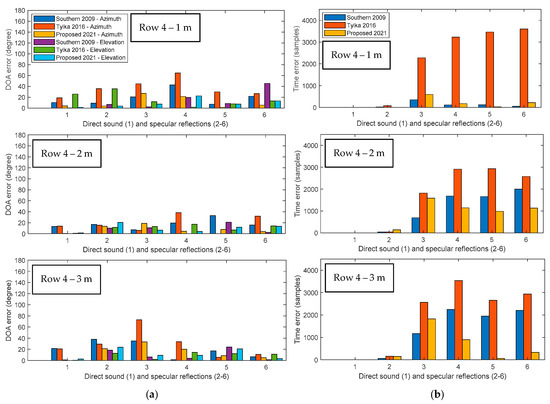
Figure 8.
Bar charts comparing the accuracy of the Southern’s method in 2009, the Tylka’s method in 2016, and the proposed DRIR interpolation algorithm in the real-world great hall arranged as shown in Figure 4b, including: (a) the error of azimuth and elevation; (b) the error of TOA. All errors are calculated as the absolute difference between the interpolated signal and the ground truth for a reference-to-known-point spacing of 1 m, 2 m, and 3 m (from top to bottom in each subplot) in row 4.
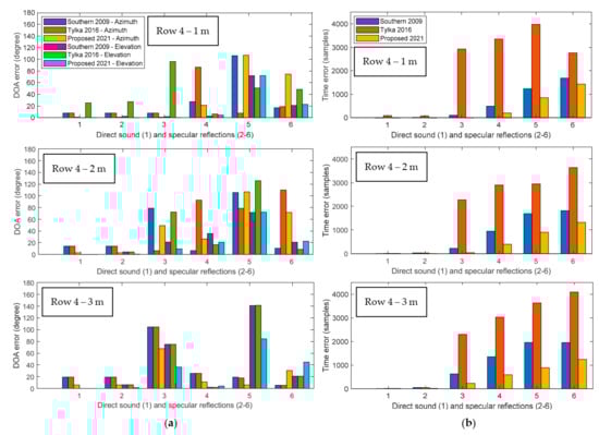
Figure 9.
Bar charts comparing the accuracy of the Southern’s method in 2009, the Tylka’s method in 2016, and the proposed DRIR interpolation algorithm in the simulated great hall arranged as shown in Figure 4b, including: (a) the error of azimuth and elevation; (b) the error of TOA. All errors are calculated as the absolute difference between the interpolated signal and the ground truth for a reference-to-known-point spacing of 1 m, 2 m, and 3 m (from top to bottom in each subplot) in row 4.
The experimental results in the simulated great hall in Figure 9 present different trends. The Southern’s method and the proposed approach show the smallest errors when the spacing is 1 m. Tylka’s algorithm presents small azimuth errors when the spacing is 1 m, whilst demonstrating large elevation and TOA errors in all cases. Generally, the proposed method leads to the smallest DOA and TOA errors. The Southern’s linear interpolation approach without DRIR decomposition also shows accurate DOA estimation, having four cases for azimuth and seven cases for elevation in Figure 9a that show the smallest error among all three comparative approaches.
4.2.2. Regular and Irregular Spacing, Row 9
The next comparison chooses positions at row 9 (the rear of the great hall) to explore the effect of the source-microphone distance and the inter-microphone distance on the DRIR interpolation accuracy. The first case selects known DRIR points at 1 m either side of the interpolation point (purple circles of Figure 4b). Another case chooses the same listening point and left DRIR as case 1, but the right DRIR is 4 m away (black circles of Figure 4b). DRIR interpolation results for these two cases in the real-world and simulated great halls are provided in the first two rows of Figure 10 and Figure 11, respectively.
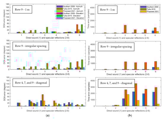
Figure 10.
Bar charts comparing the accuracy of the Southern’s method in 2009, the Tylka’s method in 2016, and the proposed DRIR interpolation algorithm in the real-world great hall arranged as shown in Figure 4b, including: (a) the error of azimuth and elevation; (b) the error of TOA. All errors are calculated as the absolute difference between the interpolated signal and the ground truth considering a 1 m regular spacing case and an irregular spacing case in row 9, and a case where the two known points and the interpolation point are located as a diagonal (from top to bottom in each subplot).
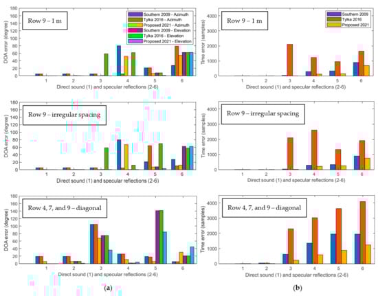
Figure 11.
Bar charts comparing the accuracy of the Southern’s method in 2009, the Tylka’s method in 2016, and the proposed DRIR interpolation algorithm in the simulated great hall arranged as shown in Figure 4b, including: (a) the error of azimuth and elevation; (b) the error of TOA. All errors are calculated as the absolute difference between the interpolated signal and the ground truth considering a 1 m regular spacing case and an irregular spacing case in row 9, and a case where the two known points and the interpolation point are located as a diagonal (from top to bottom in each subplot).
Firstly, we investigate the effects of the source-to-microphone distance on DOA and TOA estimation accuracy. By comparing the top subplot (row 9 with 1 m spacing) in Figure 10 and Figure 11 with the top one in Figure 8 and Figure 9 (Row 4 with 1 m spacing), respectively, it can be found that the DOA and TOA errors in row 9 are overall smaller than those for Row 4. Note that the proposed method shows the most consistent results in these rows in the real-world great hall. Although its error increases from row 9 to row 4, the change is not large. These results demonstrate that the further the listening position and known DRIR positions are from the source, the more accurate the DRIR interpolation will be. This argument generally holds for all the three comparative approaches. A possible explanation for this is that while row 9 is further from the source, the angular separation between the two known DRIR points used in the interpolation is smaller than that for row 4.
In Figure 11, the reduction of errors in the simulated great hall because of larger source-microphone distances is not as apparent as in Figure 10. Looking at the azimuth error in both row 9 (Figure 11) and row 4 (Figure 9), the direct sound and the first two specular reflections in row 9 are all accurate, and the Tylka’s and Southern’s methods both obtain an error of nearly five degrees. The proposed algorithm presents nearly no error in these two rows with 1 m spacing. For the fifth peak, row 9 results are smaller, but at the sixth peak, row 9 errors are much larger than that in row 4. In Figure 11a, row 9 elevation results are smaller than that in row 4 in Figure 9a but are not obvious. Only in Figure 11b are the TOA errors for row 9 significantly smaller than that in row 4 in Figure 9b.
Therefore, the proposed method and two representative DRIR interpolation approaches all perform better for larger source-microphone distances.
Analyzing results for irregular spacing for row 9 in Figure 10, it can be seen that the two cases in row 9 (regular vs. irregular spacing) have very similar results in the real-world great hall for all methods. For the same positions in the simulated great hall in Figure 11, the elevation and TOA errors for the proposed method and the Southern’s method are also similar for both cases (regular vs. irregular spacing). In contrast, the results for the Tylka’s approach show more variation for these two cases (e.g., see elevation errors of peaks 4 and 5 in Figure 11a and TOA errors of peaks 4 and 5 of Figure 11b). When analyzing the azimuth errors, results for all peaks for the Southern’s approach and the first four peaks for the Tylka’s approach are similar for the two cases in row 9 using both databases, while for the proposed method, those azimuth errors for peaks 1 to 5 are also consistent. It is worth noting that the azimuth error for the proposed method could be reduced by using an alternative DOA interpolation method that more accurately accounts for the irregular spacing (this will be future work).
4.2.3. Irregular Source-to-Microphone Distances Located Diagonally
The last setting of this experiment in the great hall is shown as green circles in Figure 4b, where the source is not right in front of the interpolation position, and there is an angle between the line of the three points and the line connecting the source and the interpolation position. The spacing is also not regular in this case. Results of DOA errors and TOA errors of the first six peaks are illustrated in the bottom row of Figure 10 and Figure 11.
In the real-world great hall in Figure 10, the proposed approach obtains the most accurate result, with all errors of DOA and TOA for the first peak close to zero, which represents the direct sound and is the main dominant component of the DRIR. The Southern’s method and the Tylka’s method show equivalent DOA errors generally, while the Tylka’s method presents slightly larger errors in terms of the TOA. In Figure 11, the simulated great hall entails large TOA errors using the Tylka’s method and large azimuth and elevation errors for all three approaches, but they all obtain accurate results in terms of elevation and TOA errors for the direct sound. As for the azimuth estimation, the proposed approach is the most accurate at the direct sound with an error of around five degrees. The largest azimuth error happens at the second specular reflection, and the Southern’s and Tylka’s methods maintain a similar error of around 100 degrees, where the proposed method also encounters an error of around 70 degrees. The large errors can also be found for the elevation at peak 5. Those large errors using all three approaches indicate their limits of dealing with such diagonally located cases, but note that their performance for the dominant DRIR component, the direct sound, and the first specular reflection are all satisfactory, particularly for the proposed method. In addition, the practical application of the proposed method only utilizes the two closest recordings having regular spacings to the listening point, the irregular scenarios provide interesting results and will be further investigated in future work.
Besides, the DRR errors are also evaluated in the great halls as shown in Table 2. Considering cases where the interpolated position is right in the middle of the two recording points with regular spacing in row 4, the proposed method and the Southern’s method obtain equivalent accuracy in the real-world great hall, with the Southern’s approach performing slightly better in the simulated great hall. In row 9 of the great hall or simulated recordings, the DRR results of the interpolated signal in both regular and irregular spacing scenarios are closer when using the Southern’s and Tylka’s approaches, while the proposed method presents smaller errors for the regular spacing case and also generally the smallest error amongst all. When it comes to the cross-row spacing conditions where recording positions in three different rows and columns are taken into account, the Southern’s method shows advantages in recovering the acoustic characteristic of DRR of the ground truth in both the real-world and simulated great halls, followed by the proposed approach. Overall, the Southern’s approach leads to the least average DRR errors in each great hall, followed by the proposed method with slight differences.
Table 2.
Comparisons of DRR errors in the real-world and simulated great halls (unit: dB).
In most of the aforementioned experimental scenarios, the proposed approach leads to the most accurate DOA and TOA estimates of the direct sound and specular reflections as well as parallel DRR accuracy to the Southern’s method. The advantages of the proposed method are mainly brought by the usage of the direction information and the decomposition of the recorded DRIR into the direct sound, individual specular reflections, and diffuse signals. By linearly interpolating the DOAs and TOA of the direct sound and early specular reflections at two known recorded positions for each unknown listening position, the DRIR signal at all listening positions can be easily obtained through synthesizing those interpolated results with one known DRIR recorded closely.
5. Conclusions
This paper has proposed an approach of DRIR interpolation for dynamically reproducing spatial audio with limited data. The DRIR is firstly represented or measured in B-format at fixed numbers of known positions. By utilizing two of these known DRIRs for each interpolation, the proposed algorithm separates the DRIR into two parts, the specular reflection (including the direct sound) and diffuse signals. A few early specular reflection signals are then further decomposed into estimated image source components and their corresponding DOAs (azimuth and elevation). Through interpolating the reflection components and the DOA at two measured positions, the useful information for reproducing the acoustic characteristic at any new position within the recording region can be obtained by synthesizing a known DRIR with the interpolated results, although this region is restricted to within the cover of available recordings due to the interpolation nature of the method.
Experiments are conducted by utilizing existing real-world recordings and our simulated recordings of the DRIR, which were designed to use the two closest recordings for interpolation, but here we have investigated broader cases with different source-to-microphone and microphone-to-microphone spacing for a thorough evaluation. Results indicate that the proposed algorithm presents the most accurate interpolated azimuth and elevation, whilst leading to the least TOA error compared with two previous representative approaches [4,16], and it works very well in a small room with an average RT (the classroom in this paper). This means the reflections in the resulting DRIR signal can be recovered precisely in terms of their directions and occurring time, which are the key to guaranteeing the DRIR interpolation accuracy and are the focus of this work. From the grid-based experiments in the same row with different regular spacing between two recorded positions, we also find that different microphone-to-microphone distances do not affect the DOA estimation accuracy much, but the TOA error is much smaller when the distance is small.
Moreover, the proposed approach shows reduced errors in two limited scenarios for conventional weighted-average interpolation methods [5]. When the listening position and known recorded points are close to the source, the conventional method from Southern [4] suffers from large errors in terms of azimuth estimation, whilst the proposed method obtains nearly zero errors in most such cases. As for scenarios of irregular spacing where the source is closer to one microphone than to the other, the proposed algorithm also obtains the most accurate estimation of the DOA and TOA among all comparative approaches. However, the errors of DOA estimation in the simulated great hall using the proposed method with irregular spacing can be large for a few specular reflections, which will cause distortions to the interpolated DRIR and affect the perception of the reconstructed spatial audio to some extent. Since these errors do not occur for the direct sound and the first specular reflection that are the main dominant components in the DRIR, the proposed algorithm can still lead to satisfactory results even when using known recordings with irregular spacing.
Additionally, DRR errors between the interpolated DRIR and the ground truth DRIR are evaluated in all aforementioned scenarios. Compared with the most accurate method from Southern, the proposed method obtains equivalent accuracy in all rooms, with slightly larger DRR errors in most cases and smaller DRR errors in a few irregular spacing cases. The reason may be related to the limits of accuracy in the signal decomposition and synthesis processes of the proposed approach. Considering all results for the DOA, TOA, and DRR, the proposed approach provides, generally, the most accurate interpolation with two known recordings each time, which suggests precise interpolated DRIRs with limited data and thus is crucial for dynamic spatial audio reproduction and VR applications.
Future work will focus on mitigating the negative effects brought by the DOA errors under irregular spacing of known recording positions in the simulated large room, further ensuring the match between two specular reflections used for interpolation, and complex acoustic characteristics of real-world rooms. Interpolation at any arbitrary listening points using more than two measured DRIRs at known positions will also be investigated, before exploring improved interpolation strategies, such as methods based on triangulation, as well as subjective metrics for evaluating the listening quality of spatial audio. In addition, the recreation and synthesis of the late reflections and diffuse components will be studied.
Author Contributions
Conceptualization, C.R. and D.J.; methodology, X.Z., C.R. and J.Z.; software, X.Z. and J.Z.; validation, J.Z.; formal analysis, C.R. and J.Z.; investigation, J.Z., X.Z. and C.R.; resources, C.R. and D.J.; data curation, J.Z. and X.Z.; writing—original draft preparation, J.Z. and C.R.; writing—review and editing, J.Z., C.R., X.Z. and D.J.; visualization, J.Z.; supervision, C.R. and D.J.; project administration, D.J. and C.R.; funding acquisition, D.J. and C.R. All authors have read and agreed to the published version of the manuscript.
Funding
This research was supported by the Electronics and Telecommunications Research Institute (ETRI) grant funded by the Korean government, grant number 20ZH1200 (The research of the basic media contents technologies).
Institutional Review Board Statement
Not applicable.
Informed Consent Statement
Not applicable.
Data Availability Statement
Data available in a publicly accessible repository that does not issue DOIs. Publicly available datasets were analyzed in this study. This data can be found here: (https://github.com/jackhong345/OpenData, accessed on 25 December 2021).
Conflicts of Interest
The authors declare no conflict of interest.
References
- Antonello, N.; Sena, E.D.; Moonen, M.; Naylor, P.A.; Waterschoot, T.V. Room impulse response interpolation using a sparse spatio-temporal representation of the sound field. IEEE/ACM Trans. Audio Speech Lang. Process. 2017, 25, 1929–1941. [Google Scholar] [CrossRef] [Green Version]
- Allen, J.; Berkley, D. Image method for efficiently simulating small-room acoustics. J. Acoust. Soc. Am. 1979, 65, 943–950. [Google Scholar] [CrossRef]
- Mariette, N.; Katz, B.F.G. SoundDelta–Large Scale, Multi-user Audio Augmented Reality. In Proceedings of the EAA Symposium on Auralization, Espoo, Finland, 15–17 June 2009. [Google Scholar]
- Southern, A.; Wells, J.; Murphy, D. Rendering Walk-through Auralisations Using Wave-based Acoustical Models. In Proceedings of the European Signal Processing Conference (EUSIPCO 2009), Glasgow, UK, 25–28 August 2009. [Google Scholar]
- Tylka, J.G.; Choueiri, E.Y. Fundamentals of a parametric method for virtual navigation within an array of Ambisonics microphones. J. Audio Eng. Soc. 2020, 68, 120–137. [Google Scholar] [CrossRef]
- Fernandez-Grande, E. Sound field reconstruction using a spherical microphone array. J. Acoust. Soc. Am. 2016, 139, 1168–1178. [Google Scholar] [CrossRef] [PubMed] [Green Version]
- Menzies, D.; Al-Akaidi, M. Nearfield binaural synthesis and Ambisonics. J. Acoust. Soc. Am. 2007, 121, 1559–1563. [Google Scholar] [CrossRef] [PubMed] [Green Version]
- Zotter, F. Analysis and Synthesis of Sound-Radiation with Spherical Arrays. Ph.D. Thesis, University of Music and Performing Arts, Vienna, Austria, 2009. [Google Scholar]
- Menzies, D.; Al-Akaidi, M. Ambisonic synthesis of complex sources. J. Audio Eng. Soc. 2007, 55, 864–876. [Google Scholar]
- Wang, Y.; Chen, K. Translations of spherical harmonics expansion coefficients for a sound field using plane wave expansions. J. Acoust. Soc. Am. 2018, 143, 3474–3478. [Google Scholar] [CrossRef] [PubMed]
- Tylka, J.G.; Choueiri, E.Y. Performance of linear extrapolation methods for virtual sound field navigation. J. Audio Eng. Soc. 2020, 68, 138–156. [Google Scholar] [CrossRef]
- Samarasinghe, P.; Abhayapala, T.; Poletti, M. Wavefield analysis over large areas using distributed higher order microphones. IEEE/ACM Trans. Audio Speech Lang. Process. 2014, 22, 647–658. [Google Scholar] [CrossRef]
- Chen, H.; Abhayapala, T.D.; Zhang, W. 3D Sound Field Analysis Using Circular Higher-order Microphone Array. In Proceedings of the European Signal Processing Conference (EUSIPCO 2015), Nice, France, 31 August–4 September 2015. [Google Scholar] [CrossRef] [Green Version]
- Samarasinghe, P.; Abhayapala, T.; Poletti, M.; Betlehem, T. An efficient parameterization of the room transfer function. IEEE/ACM Trans. Audio Speech Lang. Process. 2015, 23, 2217–2227. [Google Scholar] [CrossRef]
- Ueno, N.; Koyama, S.; Saruwatari, H. Sound field recording using distributed microphones based on harmonic analysis of infinite order. IEEE Signal Process. Lett. 2018, 25, 135–139. [Google Scholar] [CrossRef]
- Tylka, J.G.; Choueiri, E.Y. Soundfield Navigation Using an Array of Higher-order Ambisonics Microphones. In Proceedings of the Audio Engineering Society International Conference on Audio for Virtual and Augmented Reality, Los Angeles, CA, USA, 30 September–1 October 2016. [Google Scholar]
- Tylka, J.G.; Choueiri, E.Y. Models for Evaluating Navigational Techniques for Higher-order Ambisonics. In Proceedings of the Meetings of Acoustical Society of America on Acoustics, Boston, MA, USA, 25–29 June 2017. [Google Scholar] [CrossRef] [Green Version]
- Zheng, X.; Ritz, C.; Xi, J. Encoding and communicating navigable speech soundfields. Multi. Tools A 2016, 75, 5183–5204. [Google Scholar] [CrossRef] [Green Version]
- Thiergart, O.; Galdo, G.D.; Taseska, M.; Habets, E.A.P. Geometry-based spatial sound acquisition using distributed microphone arrays. IEEE Trans. Audio Speech Lang. Process. 2013, 21, 2583–2594. [Google Scholar] [CrossRef]
- Rumsey, F. Spatial audio psychoacoustics. In Spatial Audio, 1st ed.; Focal Press: Oxford, UK, 2001; pp. 21–51. [Google Scholar]
- Stewart, R.; Sandler, M. Database of Omnidirectional and B-format Impulse Responses. In Proceedings of the IEEE International Conference on Acoustics, Speech and Signal Processing (ICASSP 2010), Dallas, TX, USA, 14–19 March 2010. [Google Scholar] [CrossRef]
- Dabin, M.; Ritz, C.; Shujau, M. Design and Analysis of Miniature and Three Tiered B-format Microphones Manufactured Using 3D Printing. In Proceedings of the IEEE International Conference on Acoustics, Speech and Signal Processing (ICASSP 2015), South Brisbane, QLD, Australia, 19–24 April 2015; pp. 2674–2678. [Google Scholar] [CrossRef]
- Ma, G.; Brown, C.P. Noise Level Estimation. International Patent WO 2015/191470 Al, 17 December 2015. Available online: https://patentimages.storage.googleapis.com/19/b4/8e/389e6024f46be7/WO2015191470A1.pdf (accessed on 24 October 2021).
- Remaggi, L.; Jackson, P.J.B.; Coleman, P.; Wang, W. Acoustic reflector localization: Novel image source reversion and direct localization methods. IEEE/ACM Trans. Audio Speech Lang. Process. 2017, 25, 296–309. [Google Scholar] [CrossRef] [Green Version]
- Oppenheim, A.V.; Schafer, R.W.; Buck, J.R. Discrete-Time Signal Processing, 2nd ed.; Prentice Hall: Upper Saddle River, NJ, USA, 1999. [Google Scholar]
- Farina, A. Simultaneous Measurement of Impulse Response and Distortion with a Swept Sine Technique. In Proceedings of the 108th Audio Engineering Society Convention, Paris, France, 19–22 February 2000. [Google Scholar]
- RIR-Generator. Available online: https://github.com/ehabets/RIR-Generator (accessed on 24 October 2021).
- Ambisonics Navigation Toolkit. Available online: https://github.com/PrincetonUniversity/3D3A-AmbiNav-Toolkit (accessed on 24 October 2021).
- IoSR Matlab Toolbox. Available online: https://github.com/IoSR-Surrey/MatlabToolbox/ (accessed on 24 October 2021).
- Zahorik, P. Direct-to-reverberant energy ratio sensitivity. J. Acoust. Soc. Am. 2002, 112, 2110–2117. [Google Scholar] [CrossRef] [PubMed]
Publisher’s Note: MDPI stays neutral with regard to jurisdictional claims in published maps and institutional affiliations. |
© 2022 by the authors. Licensee MDPI, Basel, Switzerland. This article is an open access article distributed under the terms and conditions of the Creative Commons Attribution (CC BY) license (https://creativecommons.org/licenses/by/4.0/).