Locating Image Sources from Multiple Spatial Room Impulse Responses

Abstract

Measured spatial room impulse responses have been used to compare acoustic spaces. One way to analyze and render such responses is to apply parametric methods, yet those methods have been bound to single measurement locations. This paper introduces a method that locates image sources from spatial room impulse responses measured at multiple source and receiver positions. The method aligns the measurements to a common coordinate frame and groups stable direction-of-arrival estimates to find image source positions. The performance of the method is validated with three case studies—one small room and two concert halls. The studies show that the method is able to locate the most prominent image sources even in complex spaces, providing new insights into available Spatial Room Impulse Response (SRIR) data and a starting point for six degrees of freedom (6DoF) acoustic rendering.

1. Introduction

Measuring a room impulse response (RIR) with a microphone array makes analyzing sound event directions possible. Thus, a Spatial Room Impulse Response (SRIR) can be analyzed in both temporal and spatial domain, which helps us to understand the acoustics of a room better and allows us to reproduce the acoustic behavior of the measured space faithfully. Parametric methods for processing SRIR, such as the Spatial Decomposition Method (SDM) [1], Spatial Impulse Response Rendering (SIRR) [2] or Higher-order SIRR (HO-SIRR) [3], have been a cornerstone of concert hall research in recent years [4,5]. Such techniques have enabled us to directly compare different spaces in numerous listening tests. Besides auralizing the SRIRs, extracted directional parameters have been used early on to visualize reflections [6]. Broadband direction estimates are especially well-suited for this, since they allow for interpreting reflections from large walls as image sources with a specific location in space. Such visualizations have been used, for example, to better understand the results of perceptual tests [7].

However, existing parametric SRIR methods have only used individual measurement positions, whereas the feasibility of detecting individual reflections based on one measurement is limited. It depends on several factors, such as estimation accuracy, separability of reflections that arrive in short succession, and the visibility of specific reflections in complex room geometries. Therefore, we propose to extend broadband SRIR processing to make use of multiple source and receiver positions at once, combining several SRIR measurements in order to locate image sources more reliably. By doing so, the proposed technique enables improved localization of image sources. While it would be possible to use these as a basis for multi-perspective auralization, this paper only focuses on detection and localization from several real measurements.

The article is organized as follows—we introduce all the processing stages of our method in Section 2. We then present the analysis of a medium sized room and two concert halls in Section 3. For a rectangular room, we show the results of the analysis with five source positions. Then, we extend the analysis to more complex cases and demonstrate that combining the directional estimates of several SRIR measurements can give new insights into available concert hall data. Finally, we discuss properties as well as applications of the proposed methods and draw conclusions.

2. Methods

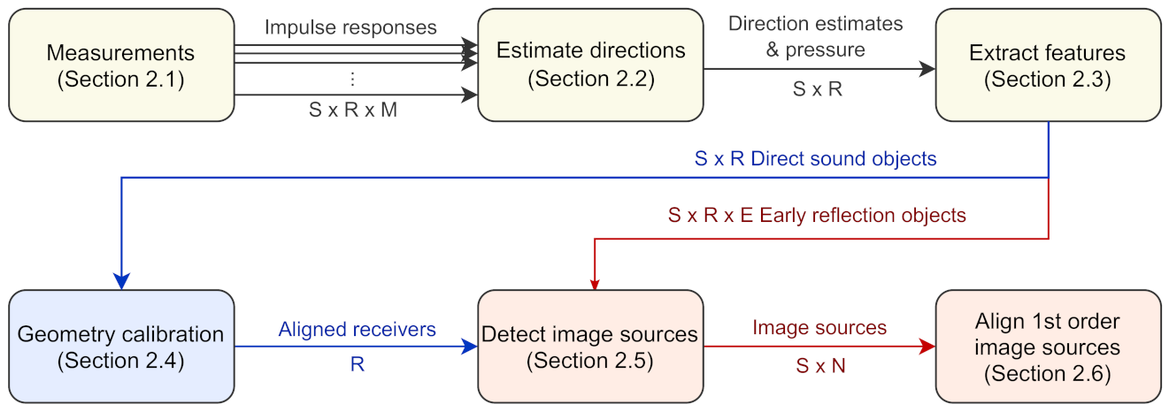
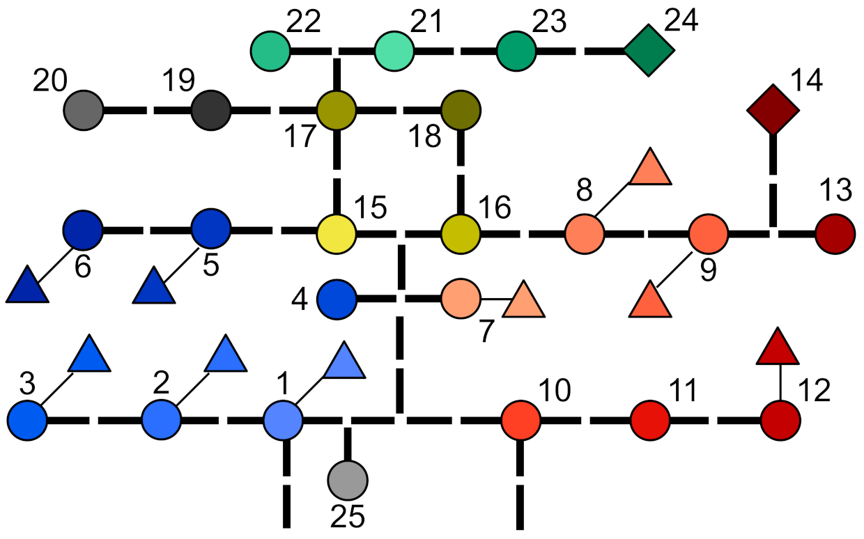
This section introduces the complete image source detection method illustrated in Figure 1. The method is divided into six stages. The first stage involves conducting several SRIR measurements between multiple sources and receivers in the space of interest. Next, the measured responses are analyzed to obtain sample-wise direction estimates. In the third stage, direct sound and early reflections are identified in each response. Together with two features predicting reliability, each detected early reflection forms an early reflection object (ER object). For the fourth stage, the direct sound estimates are sent to the geometry calibration stage, which uses the data to determine the source-receiver layout. Once the layout is known, the fifth stage combines the ER objects to estimate image source locations of each sound source. In the last stage, multiple sources can be translated to the same location in order to visualize first order image sources even more clearly.

2.1. Measurements

The image source detection algorithm uses multiple SRIR measurements between different source and receiver positions. As in a single-microphone RIR measurement, a sound source plays a logarithmic sweep that is recorded by a receiver microphone array. The recorded signals are then convolved with the time-inverted sweep [8] in order to obtain a set of RIRs from the array. One SRIR measurement therefore contains a set of RIRs between one source and one receiver position, which we call source-receiver measurement.

In the presented case studies (Section 3), SRIRs have been measured with a GRAS 50VI-1 intensity probe. It consists of six omnidirectional capsules in a symmetric layout, with one pair of capsules on each coordinate axis. The probe is well suited for directional estimation based on the time difference of arrival (TDoA). The later processing stages also require an omnidirectional pressure response. The intensity probe obtains this response from the topmost microphone, although the most optimal solution would be to acquire it from the center of the array [9].

Apart from performing the impulse response measurements themselves, one needs to perform a few geometrical measurements to establish the absolute frame of reference for geometry calibration (Section 2.4). For the method described here, we use manually measured source positions and determine the receiver positions automatically from the direct sound estimates. If the source positions are kept static, one can move around the space with the receiver array freely. Best results have been observed when the loudspeaker is rotated to always point towards the microphone array. The geometry calibration algorithm used here can compensate for small inaccuracies in the receiver array orientation, but generally one should orient the microphone array consistently w.r.t. the frame of reference between measurements.

The geometry calibration algorithm does not require sample-wise synchronization of source and receiver. Anyhow, one can determine the measurement system delay (Section 2.4.1) by measuring the input-output delay of the audio card, using a loop-back connection. But even after compensating this, there can still be some uncompensated system delay left, for example, due to digital signal processing in the amplifier and mechanical group delay in the loudspeaker. For this reason, the presented geometry calibration algorithm (Section 2.4.2) does not use the measured time information directly, but attempts to estimate any constant delay. While even other methods could be used to improve synchronization during measurement, using legacy datasets clearly demands for the algorithm to solve this problem. To avoid another bias, one can approximate the speed of sound accurately enough from measuring the air temperature.

2.2. Estimate Directions

The directional estimation stage aims at determining the sample-wise Direction-of-Arrival (DoA) for each source-receiver measurement. To do so, we employ the directional analysis algorithm found in the SDM —a parametric SRIR processing method that uses a broadband directional estimate for every sample of the response. It has first been introduced by Tervo et al. [1] and is distributed as a MATLAB toolbox [10]. The algorithm can use any microphone array with at least four 4 microphones that are not in the same plane. In addition to the DoA estimates, also an omnidirectional response h is needed for further processing. In case the used microphone array is comprised of omnidirectional receivers, simply one of the microphones is used. It is important to note that the particular estimation method operates immediately on the responses measured by a microphone array (A-Format). Nevertheless, also spherical harmonics domain (B-Format) responses could be processed by using a different directional estimator.

As an input, the directional analysis takes a set of M impulse responses ${\mathbf{h}}_{i,j}\left[n\right]$ measured by each of the R receiver microphone arrays in response to each of the S sources. The method then segments the responses into blocks of N samples with a hop size of one sample, and computes the cross-correlation between all microphone pairs. For instance, 15 correlation functions are obtained for the six-capsule open array used in this study. After applying Gaussian interpolation to each cross-correlation function, the location of its highest peak reveals the TDoA between the corresponding microphone pair. The DoA of the strongest sound event in the analysis block is computed from all TDoAs and the known microphone positions within the array. This way, each source-receiver measurement is associated with the DoA estimate ${\mathbf{u}}_{i,j}\left[n\right]$ for each sample n.

The minimum possible length of the analysis block is determined by the spatio-temporal limit $\Delta T_{min}$, that is, the time difference at which two reflections can still be separated. This limit is proportional to the largest distance within the receiver array $l_{max}$ [1]:

$$\begin{array}{c}\hfill \Delta T_{min}=\frac{2l_{max}}{c_0},\end{array}$$

(1)

where $c_0$ is the speed of sound inside the measured room. For instance, the measurement array in Section 3.1 has $l_{max}=5$ cm, which corresponds to a spatio-temporal limit of $\Delta T_{min}\approx 0.29$ ms. In practice, window sizes are selected to be even slightly larger $N=\Delta T_{min}{f}_s+C$ (with some constant C) in order to stabilize the DoA estimates. Of course, the increased stability comes at the cost of a lower time resolution. This means that the selected block length limits the separability of reflections. Should two or more reflections arrive at the array within the same analysis block, they cannot be separated reliably.

Clearly, apart from the room geometry, the Time-of-Arrival (ToA) of reflections depends on the source and receiver positions. In rooms with simple geometries, one can try to set up sources and receivers so that at least the first-order reflections are separated well in time, and not more than one reflection falls within one analysis block. For example, if either source or receiver is placed at the center of the room, the symmetry axes of the room should be avoided for the counterpart. For rooms with more complex geometries, attempting such informed placement represents a larger effort and makes the measurement-based detection of reflections obsolete. Hence, it must be assumed that some individual reflections fall below the spatio-temporal limit and cannot be detected reliably, especially in small rooms. In these cases, one greatly benefits from the proposed measurement combination algorithm. By using multiple receiver positions, it is less probable that the same reflections overlap in all positions. This in turn increases the probability of detecting the true direction of each individual sound event.

2.3. Extract Features

Although the SDM analysis provides DoA estimates for all RIR samples, it does not reveal which estimates are reliable or belong to either the direct sound or early reflections. Both of these properties are hard to determine from the RIR and DoAs directly. For this reason, it is easier to first extract features from the SDM data and then identify the reliable sound events.

The potential early reflections are identified based on the sound level peaks in the RIR. To do this, one extracts two features at each peak, namely peak prominence and DoA stability. Then the peaks are separated to direct sound and early reflection peaks. Finally, the early reflection peaks are filtered according to a certain prominence and stability level. Only the peaks fulfilling both criteria are passed on to the later processing stages. Note that the number and the type of features predicting stability could easily be modified, for example to match a modified directional estimation algorithm.

Naturally, one needs to determine the sound level peaks first in order to extract features at their locations. The peaks are determined from sound level L of the RIR, calculated as

$$L\left[n\right]=10lg\left(\sum _{k=1}^{N}h{[k+n-(N/2)-1]}^2{\mathit{g}}_N\left[k\right]\right),$$

(2)

where n is the sample index, h is the selected omnidirectional RIR and ${\mathit{g}}_N$ is a Gaussian window of length N. ${\mathit{g}}_N$ is normalized so that the sum of its samples is equal to 1. The signal peaks are then defined as the samples that have higher value than their neighbors. Next, the noise is discriminated from the signal by applying an onset threshold, dropping any peaks from the beginning of the response that do not exceed a set sound level value. In this paper, the applied onset thresholds range between −16 and −10 dB w.r.t. the maximum sound level depending on the room.

The remaining peaks are then passed to the actual feature extraction. The first feature that is extracted is peak prominence (a.k.a. topographic prominence). It indicates how distinct the sound level peak is from the rest of the response. A prominent peak is either higher than any other peak or is separated from other prominent peaks by low signal values. In turn, peaks with low prominence either do not raise from the signal baseline much or are located at the slopes of more prominent peaks. In practice, peak prominence (in dB) is determined with the following procedure:

1.

Denote the current peak as A.

2.

Search for peaks preceding or following A that have higher sound level than A has. Select the closest two and denote those as B and C. In case there is no higher peak in either direction, select the start or end of the signal.

3.

Get the signal minima of intervals [B, A] and [A, C] denoted as B${}_{min}$ and C${}_{min}$, respectively.

4.

Peak prominence of A is $max({\mathbf{B}}_{min},{\mathbf{C}}_{min})$.

The second feature, DoA stability, represents how static the direction estimate is around the sound level peak. The DoA sample is considered stable if it stays within a certain angular range compared to the DoA at the peak. In other words, it indicates that the peak likely belongs to a single plane wave, that is, one specular reflection. On the contrary, unstable estimate hints that the DoA is affected by multiple sound events at the same time.

The DoA stability is calculated by first comparing the central angle between the DoA estimate of the sound level peak ${\mathbf{u}}_{}\left[k\right]$ and the DoAs right before and after it. Next, the angle is compared to a pre-defined angle threshold in order to get a binary result. In short, these two steps can be presented together as follows:

$${\mathbf{p}}_k\left[n\right]=\left\{\begin{array}{cc}1,\hfill & arccos{\mathbf{u}}_{}^{\mathrm{T}}\left[k\right]{\mathbf{u}}_{}\left[n\right]<{\alpha }_t\hfill \\ 0\hfill & \mathrm{otherwise},\hfill \end{array}\right.$$

(3)

where ${\mathbf{u}}_{}\left[n\right]$ is the nth DoA sample in the impulse response and ${\alpha }_t$ is the user-selected angular threshold (in this paper, ${\alpha }_t=1^{\circ }$). The selected samples then form a stable sample interval. The samples in the interval stay within ${\alpha }_t$ and have no 0-valued samples between them and the peak. The DoA stability descriptor is equal to the duration of the stable sample interval.

After calculating the features, the sound level peaks and their feature descriptors are divided into direct sound and early reflections. Direct sound is selected from the peaks that arrive up to 1 ms after the first detected peak. By considering several peaks, the direct sound can be detected robustly even if the direct sound would not be the highest pressure peak in the response, which can easily happen if the source is pointing away from the array. The rest of the direct sound peaks are discarded, and the peaks after 1 ms are treated as early reflection candidates.

Next, the early reflection candidates must meet certainty thresholds for peak prominence and DoA stability. Selecting the two thresholds require a trade-off. Higher thresholds filter out more false positive detections, while lower thresholds find less prominent early reflections. For peak prominence, a suitable threshold was found to be 10 dB, whereas the DoA stability threshold was set to a 50 $\mathsf{\mu }$s. These thresholds were found to reduce noise drastically while still maintaining a reasonable sensitivity for less prominent early reflections. Finally, if a peak exceeds both limits, it is assumed to belong to an early reflection.

In the last step, the feature descriptors are combined with additional data that describe other sound event properties. The additional data consists of the ToA, DoA and sound level of the peak. The DoA is an average of the DoA samples in the stable sample interval, which is expected to reduce the measurement noise in the location estimate. The described data form either a direct sound or an ER object, depending on what kind of sound event it is describing. In the following stages, direct sound objects are utilized to align the measurements and ER objects to find the actual image sources.

2.4. Geometry Calibration

The previous sections have described how direct sound and early reflection estimates are extracted from each source-receiver measurement. Up to this point, the data from each receiver is presented in its own coordinate frame. Yet, in order to estimate the image source positions from multiple measurements, the data needs to be transformed into a global coordinate frame. To do so, one needs to have knowledge of the receiver orientations and positions in the global frame.

There are several options for identifying the receiver layout, requiring different amounts of information. On one hand, there is the option to measure all positions and orientations manually. For a large number of receivers, this approach is laborious and susceptible to measurement errors. In our experience, measuring the array rotation with high accuracy is especially difficult in practice. On the other hand, there are fully automatic microphone array geometry calibration approaches using, for example, DoA, ToA or TDoA information [11]. If the measurement system delay was not determined or contains errors, the ToA is easily biased. However, an unbiased DoA estimate of the direct sound from each source to each receiver is readily available, so one could use DoA-based microphone array calibration methods. Algorithms for calibration in 2D were presented in [12,13], and could be extended. Such DoA-based approaches typically rely on non-linear least squares optimization and have strong similarities to photogrammetry. There, multiple pictures of the same scene allow for creating a 3-dimensional reconstruction, which requires estimation of the camera positions and orientations. The advantage of DoA-based automatic calibration is that it is sufficient to measure 3 source or receiver positions manually. Moreover, it does not depend on ToA information, which might suffer from the mentioned systematic biases.

For the data presented here, we applied an approach that relies on measuring only the source positions manually. In practical measurements, this requires significantly less effort than measuring all positions. The receiver positions are computed from the direct sound DoAs.

Apart from the receiver positions, the geometry calibration stage also determines the ToA bias explicitly. This is not only important for the geometry calibration itself, but also for the image source estimation stage, as the biases described next apply to all sound events.

2.4.1. Time-of-Arrival Bias

Knowing the ToA enables estimating the distance of a sound event. In this way, the ToA of the direct sound helps to determine the array geometry. Additionally, the ToAs associated with the ER objects are ultimately used to estimate the image source positions in space. However, determining distances based on the ToA data is easily biased by errors in the assumed speed of sound $c_0$ and any uncompensated measurement system delay $t_e$. Depending on the actual distance of the sound event $d_i$ and the speed of sound $c_0$ during the measurements, the ToA of the sound event $t_i$ will be registered as

$$t_i=\frac{d_i}{c_0}+t_e,$$

(4)

where $t_e$ is the measurement system delay biasing the ToA. When translating this measured ToA back into its associated travel distance, using the assumed speed of sound c will in turn bias the travel distance estimate $d_i^{\prime }$:

$$d_i^{\prime }=\frac{c}{c_0}{d}_i+c{t}_e.$$

(5)

Clearly, the errors have different effects on the reconstructed travel distance $d_i^{\prime }$. While the measurement system delay adds a constant distance bias, a ratio of assumed vs. real speed of sound scales the distance.

The scale of the two biases is very different. Usually, the speed of sound deviation does not affect the result much. By default, the SDM toolbox [10] fixes c to 345 m/s, while $c_0$ varies between 343.8–347.2 m/s in regular room conditions (20–25.5 ${}^{\circ }$C, 1013.25 hPa, 50 % Rh) [14]. This means that the deviation between them varies only $\pm 2\mathrm{m}/\mathrm{s}$, which is small w.r.t. the speed of sound itself. This error is negligible for small rooms, but it starts to take effect with longer distances. For example, the farthest distance seen in the concert hall data presented in Section 3 is roughly 35 m, which would result in a difference of about $\pm 20\mathrm{cm}$. In contrast to that, the measurement system delay heavily impacts the estimation of small distances. For instance, a 2 ms delay on the signal onset corresponds to roughly a 69 cm offset on the measured sound event distance, independent of $d_i$.

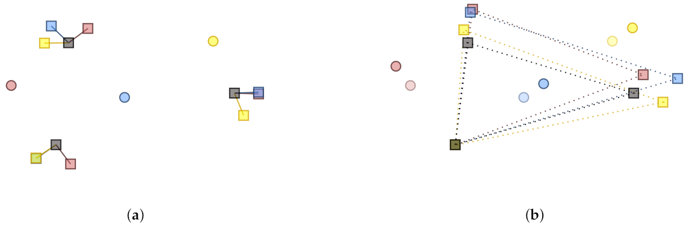
The biased travel distance causes position-dependent warping of the detected measurement layout. This phenomenon has been illustrated in Figure 2. There, three receivers (red, blue and yellow circles) have been set up to measure three sound sources (grey rectangles). Each receiver has managed to capture the DoAs correctly, but the ToA has been biased by constant delay of the sound sources. Therefore, each receiver has located the sound source further away from the measurement point than what it actually is (colored rectangles). This affects the detected shape of the sound source array. For this very reason, one cannot apply a simple rigid-body fit to find the receiver array orientations, which can only identify a common rotation, translation and scaling. When the rigid-body fit finds the optimal rotation and translation based on the warped array, the position and orientation of the receiver are not accurate. Accordingly, it is necessary to compensate for the delays first.

2.4.2. Delay-Compensated Fit

Delay-compensated fit is a method that transforms receiver data to a common coordinate frame. The method consists of two steps. In the first step, one uses the estimated direct sound DoA data and the manually measured source reference positions to estimate the measurement system delays. With the delays at hand, one then approximates the corrected sound source positions relative to each receiver. The second step then applies rigid-body fit to these positions to approximate the receiver orientation. The orientation in turn affects the DoAs, which enables iteratively improving the result.

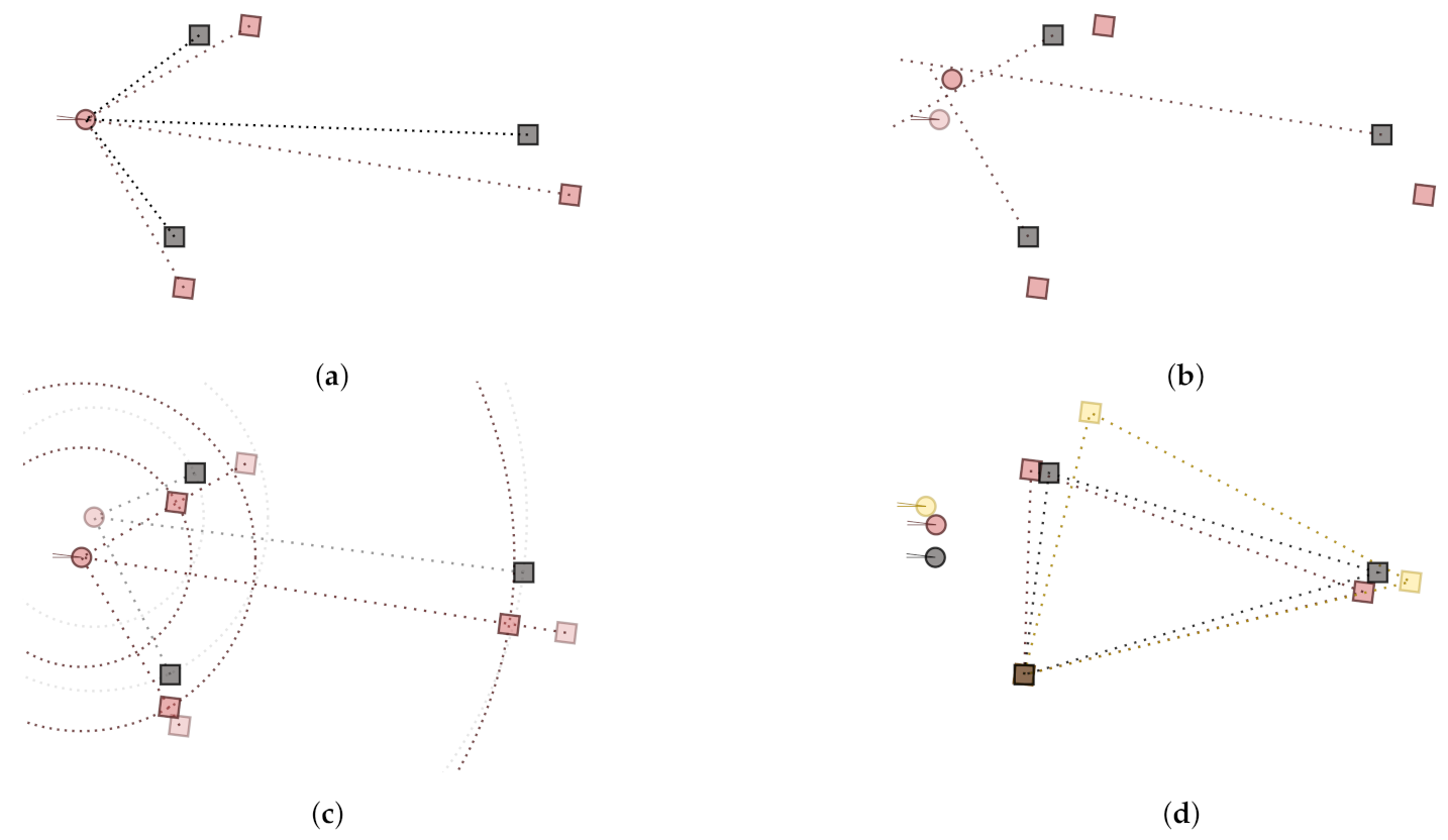
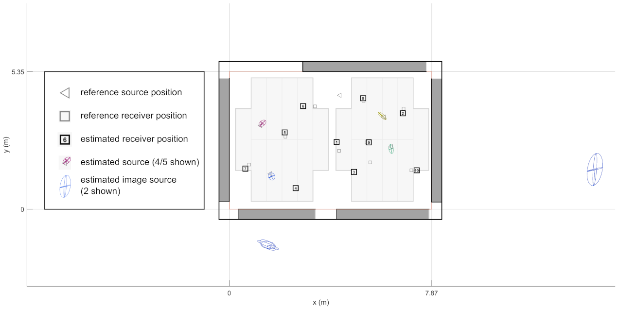
The first step of the delay-compensated fit is illustrated in Figure 3. As a starting point, one knows the reference sound source positions (in grey). Slight rotation of the receiver during measurement and the measurement system delay causes the estimated positions (red squares) to be mislocated from their actual positions.

There are two steps in approximating the measurement system delay. The first step estimates the receiver position from the direct sound DoAs. This is done by generating lines from source positions and their corresponding DoAs and by resolving the closest point to those lines [15]. The second step then approximates the measurement system delay $t_{e,i,j}^{\prime }$ based on the found receiver position as

$$t_{e,i,j}^{\prime }=\frac{\left|\right|{\mathbf{s}}_{0,i}-{\mathbf{r}}_j\left|\right|-\left|\right|{\mathbf{s}}_i-{\mathbf{r}}_j\left|\right|}{c},$$

(6)

where ${\mathbf{s}}_i$ and ${\mathbf{r}}_j$ are the approximated positions of sound source i and receiver j, receiver j and sound source i, respectively; ${\mathbf{s}}_{0,i}$ is the reference position of the sound source i; and c is the assumed speed of sound. Removing these approximated delays practically sets the distance of the approximated source to correspond to the reference source distance from the approximated receiver position. This in turn nudges the detected source array shape closer to the actual shape, see Figure 3. The corrected shape effectively improves the chances to fit the array correctly with the rigid-body fit.

The second step applies the rigid-body fit to the distance-corrected measurement data. With rigid-body fit we refer to partial Procrustes analysis, which determines rotation and translation between two point sets [16]. Reorienting the receiver according to the result leads to rotation of all associated DoA data, which can be used in the next iteration to approximate the measurement system delay again.

Undoubtedly, there may also be errors in the measured DoAs that have to be treated accordingly. Here, the treatment is implemented by applying Monte Carlo cross-validation. Instead of fitting the data w.r.t. all reference source positions, only a subset of positions are used at a time. Each receiver is fitted multiple times to three or more randomly selected reference positions. The results form fit candidates that are then evaluated by the error measure $\mathit{f}$. It compares the source positions implied by the fit to the position that were measured manually

$$\mathit{f}=\sum _{i=1}^S\left|\right|{\mathbf{s}}_i-{\mathbf{s}}_{0,i}{\left|\right|}^2.$$

(7)

Finally, the fit candidate with the lowest $\mathit{f}$ is selected as the actual position and orientation of the source.

2.5. Detect Image Sources

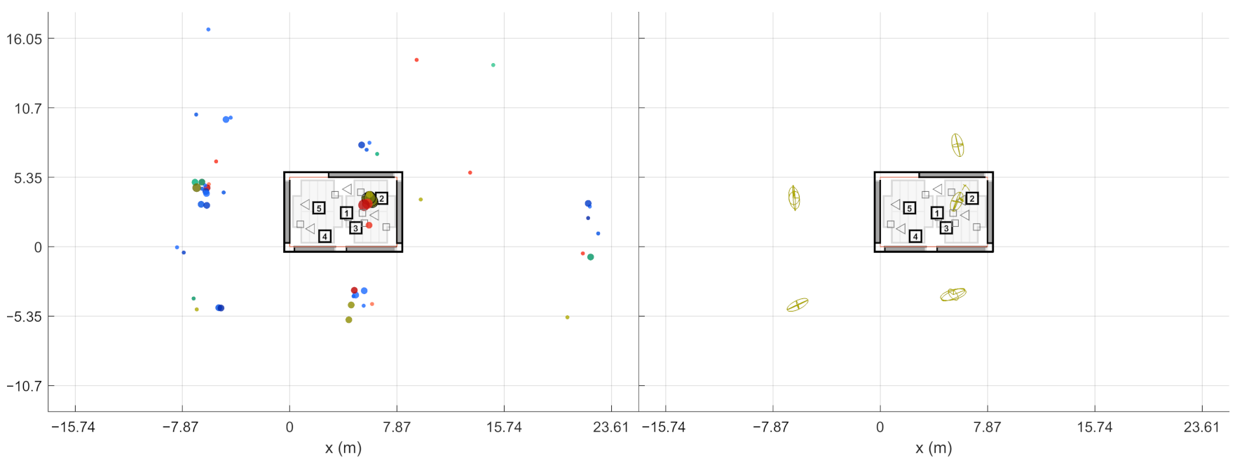
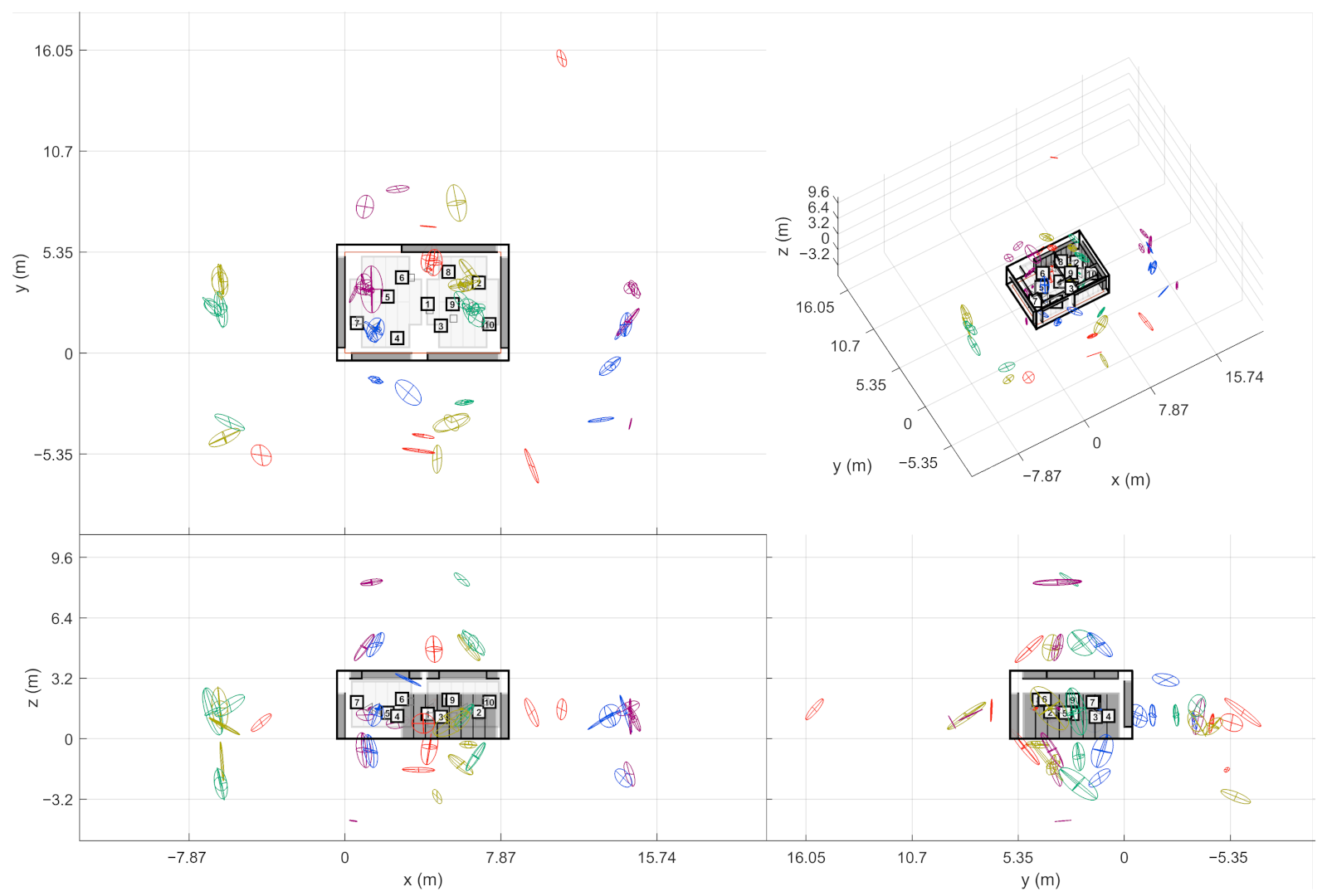
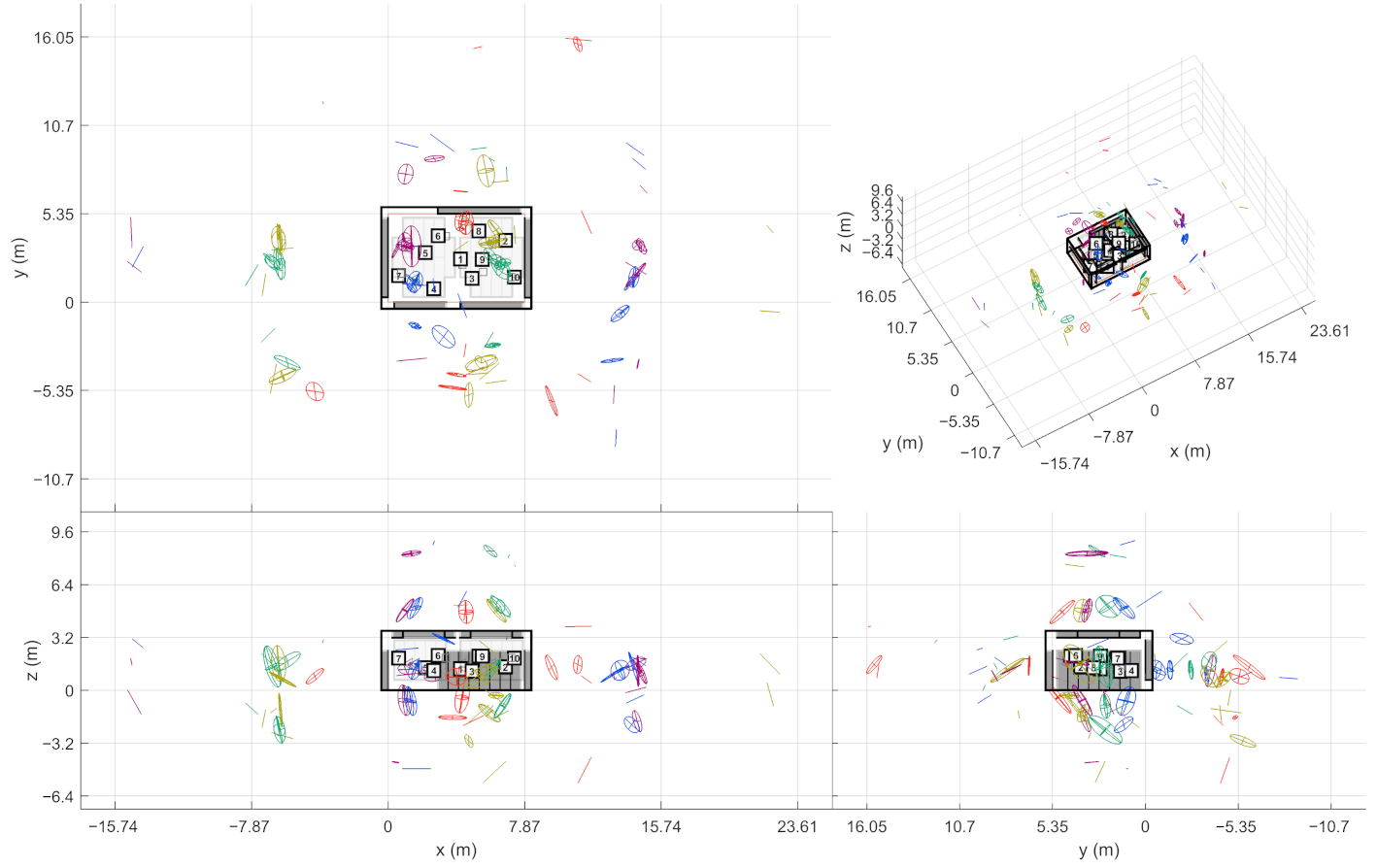
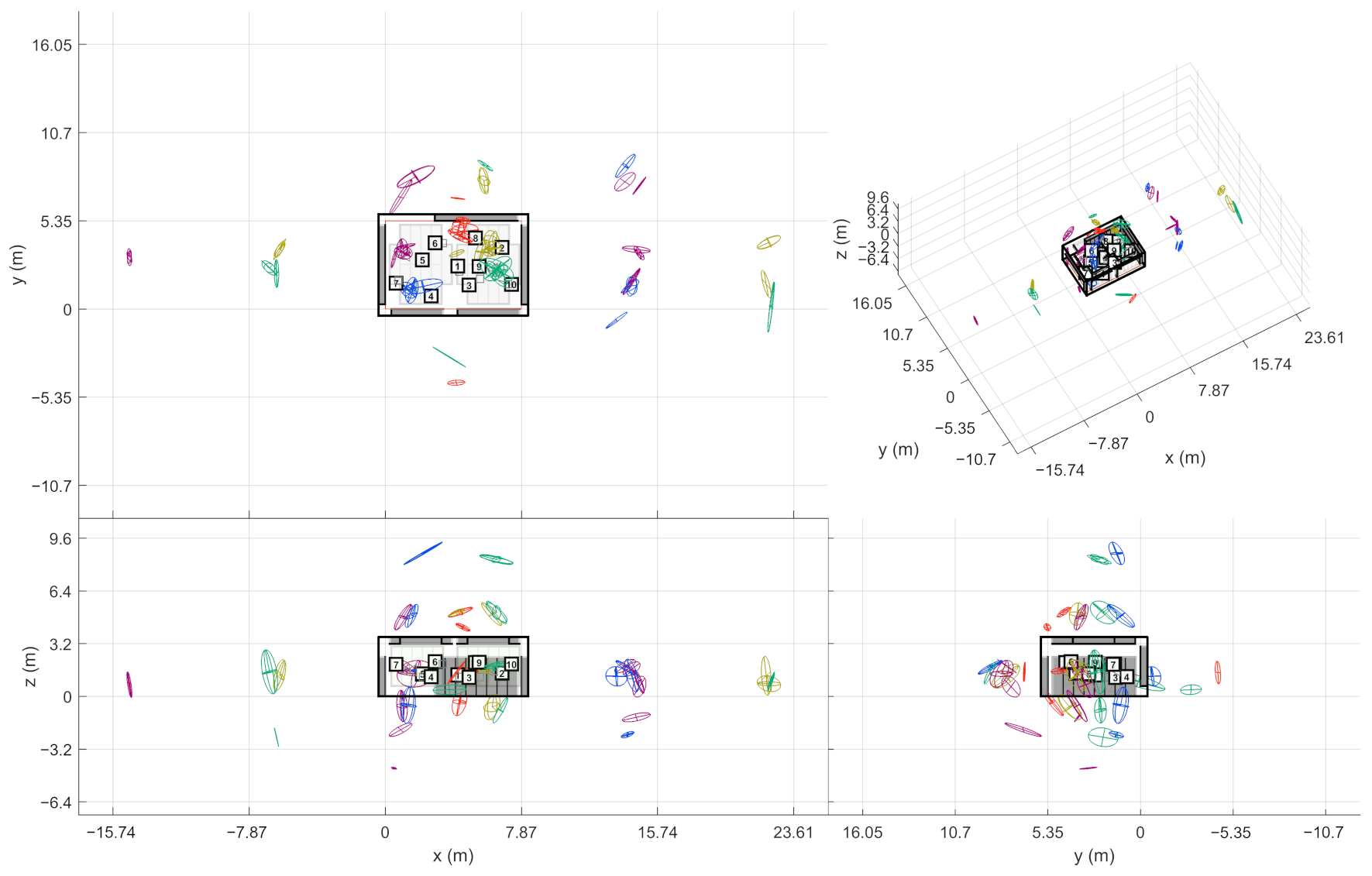
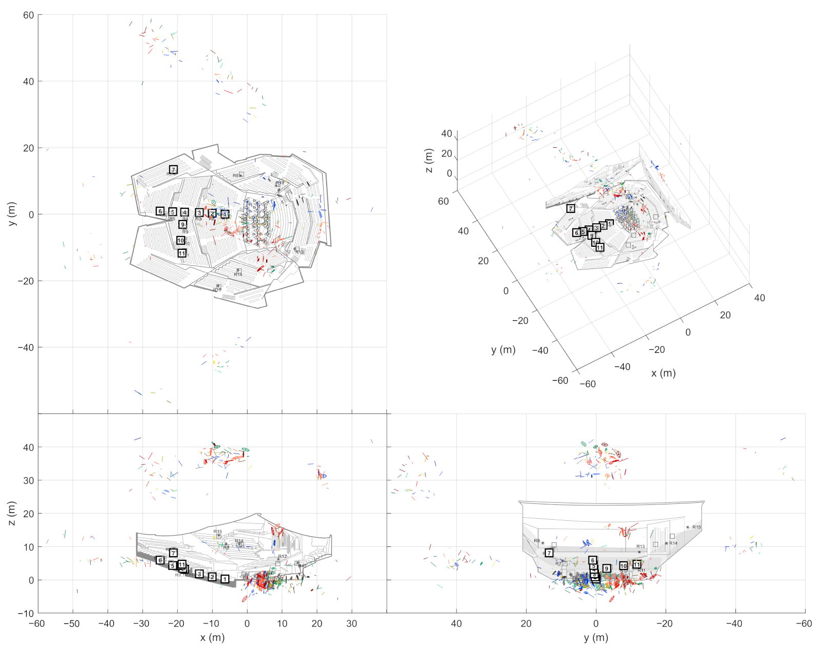
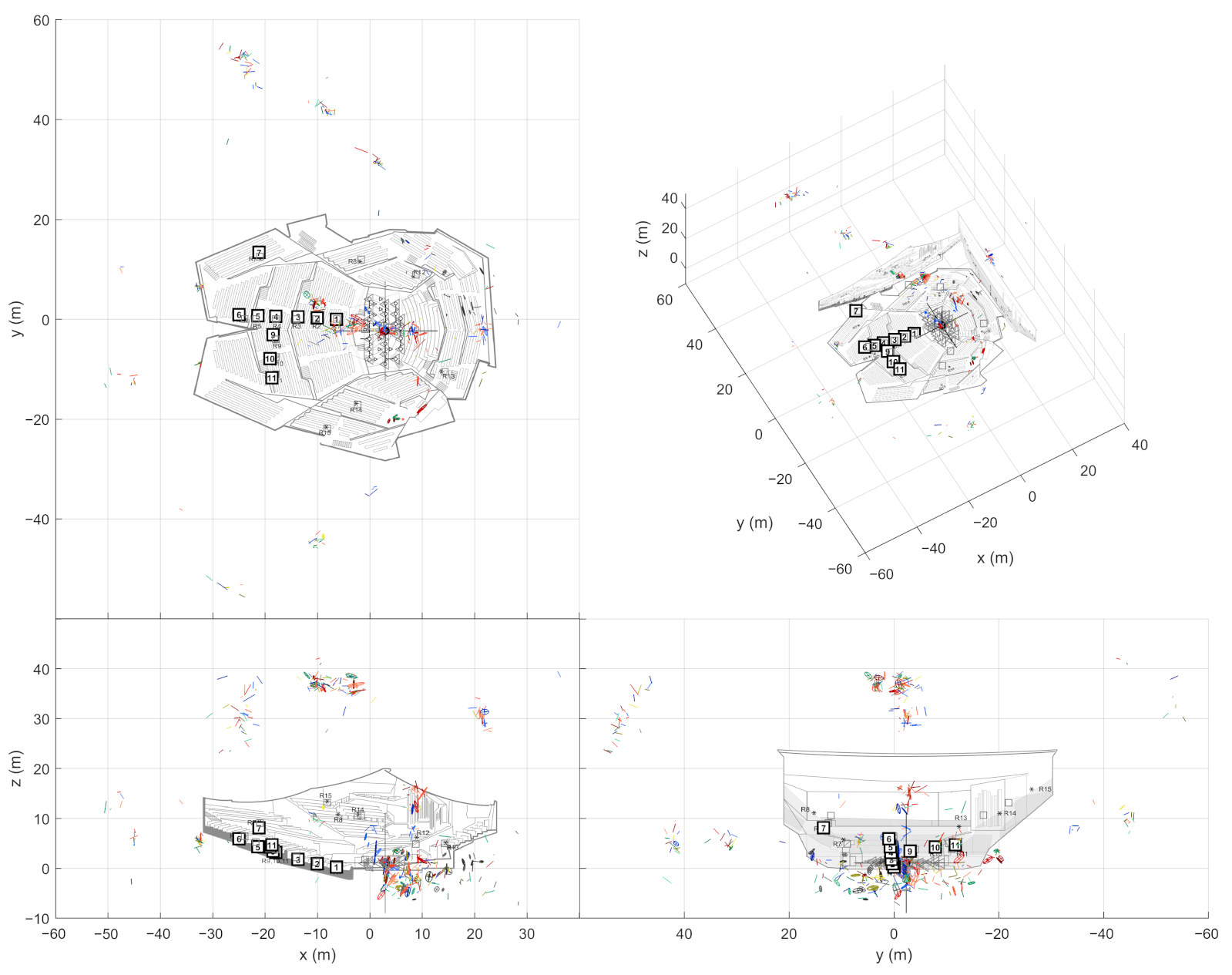
At this point, the source-receiver measurements have been aligned to the world coordinate frame. This way the extracted ER objects are also comparable w.r.t. each other. In other words, the ER objects from one sound source should be located close to each other if they have been reflected from the same planar surface. In theory, the ER objects from multiple receivers should gather around the approximate image source positions when presented in the common coordinate frame. However, not all receivers report the same image sources, and some of the objects might still be false detections, as shown on the left in Figure 4. As shown on the right, combining the receiver data not only allows finding more reflections than it is possible with a single measurement, but also manages to filter out additional false detections. Therefore, the next step is to detect image sources by clustering the extracted ER objects.

The stage presented here aims at creating multivariate Gaussian distributions out of ER objects. For each sound source, the ER objects from associated source-receiver measurements are clustered with the so called Density-Based Spatial Clustering of Applications with Noise (DBSCAN) algorithm [17] (grouping distance 1 m (Euclidean), min. 2 neighbors to consider as a core point). After this, each cluster selects one ER object per receiver that has the highest sound level. If the cluster still contains ER objects from a defined number of receivers, they form an image source. The required number of receivers is an important tuning parameter that allows a trade-off between detection noise and precise image source locations.

The found image source is presented as a multivariate Gaussian distribution that is weighted by DoA stability of the ER objects. The distribution mean is considered as the actual image source location and the covariance as the reliability of the location estimate. This way, each image source is not only presented as a point in space but as a volume where the actual image source most probably resides in.

2.6. Align 1st Order Image Sources

The algorithm has now found the image sources for all the sound sources in the scene separately. However, when the results are plotted, the multiple source positions also spread the image sources to a large volume. This may merge two image source locations that are located close to each other, effectively obscuring some of the potential findings from plain sight. For visualization purposes, it is therefore beneficial to translate the image source data to share a common source point. By doing this, single image sources are occupying a smaller volume, effectively improving separability.

The image sources are translated in the following way. First, one sets the origin of the new coordinate system; here, the origin is selected as the mean of the measured sound source positions. The origin determines the translation ${\mathbf{t}}_i$ for each sound source position ${\mathbf{s}}_i$. The translated image source positions ${\tilde{\mathbf{s}}}_{i,n}^{\prime }$ are then calculated as follows:

$${\tilde{\mathbf{s}}}_{i,n}^{\prime }={\tilde{\mathbf{s}}}_{i,n}+{\mathbf{t}}_i-2\left({\mathbf{t}}_i·{\mathbf{n}}_{i,n}\right){\mathbf{n}}_{i,n},$$

(8)

where ${\tilde{\mathbf{s}}}_{i,n}$ is the original image source position and ${\mathbf{n}}_{i,n}$ is the unit vector between ${\tilde{\mathbf{s}}}_{i,n}$ and ${\mathbf{s}}_i$. In other words, one assumes a reflecting wall between the real source and the image source. When the real source is moved, the movement towards and away from the wall is reflected for the image source while the parallel movement stays unaffected. The operation is also identical to assuming that all found reflections are first order image sources. Even though this is not always the case, the real first order image sources are hypothesized to converge to a clear reflection groups.

3. Case Studies

The performance of the presented algorithm was evaluated with three different spaces. The first space was selected to be a rectangular room equipped with variable acoustics panels on the walls and the ceiling. This way, it was comparatively easy to test how the room acoustics affect the performance of the algorithm. In addition to this room, the method was applied on two concert hall datasets. Both of the halls were complex in shape, thus considered to represent challenging applications properly.

The algorithm output for the cases is illustrated in Appendix A, Appendix B and Appendix C. All the plots use the same format where the space is shown from three perspectives: plan (x-y), section (x-z) and transverse (y-z). Additionally, a three-dimensional image is provided to allow the reader to understand the relations of the three plots.

All the plots follow the legend illustrated in Figure 5. The plots use four different markers to illustrate the results. The source and receiver positions measured on-site are depicted with grey triangles and rectangles, respectively. From these two, only source positions were used as a reference in the algorithm; the shown receiver positions have been plotted solely to evaluate the fitted receiver positions shown as numbered rectangles. In addition to these three markers, the estimated source position and image sources are illustrated with colored markers. The color of the marker defines the source, whereas the marker crosshair and size describe the mean and covariance of the sound event; the larger the marker, the more uncertain the position estimate is. In addition to the aforementioned markers, the plots with a centered source (Section 2.6) use a black crosshair to mark the centered source position.

3.1. Variable Acoustics Room Arni

As a proof of concept, the algorithm was first applied on a variable acoustics room Arni located at the Aalto acoustics laboratory. The room has a rectangular shape (dimensions $7.9\times 5.4\times 3.2$ m) and has 55 variable acoustics panels installed on the walls and in the ceiling. The panels can be opened and closed individually, that is, the section of the surface becomes either absorptive or reflective. When all panels are closed, the reverberation time of the room is 1.6 s at mid frequencies; and when opened, the reverberation time drops to 0.4 s. These properties allow us to test the algorithm in different acoustic conditions without changing the measurement setup.

The measurements were carried out as outlined in Section 2.1. As sound sources, 5 loudspeakers (model: Genelec 8331A) were set up around the room. They were oriented so that all of them pointed to the center of the room. The acoustic centers of the loudspeakers were measured w.r.t. the front faces of the panels and the floor, resulting in reference source positions. SRIRs were then measured for 10 receiver positions with a GRAS VI50-1 vector intensity probe (spacer size 5 cm). Apart from one receiver, these positions were also documented to better evaluate the algorithm performance. The SRIRs were recorded with a custom MATLAB-based recording software [18] and analyzed by the algorithm described in Section 2. The image source search results are presented in Appendix A.

Figure A1 visualizes the fit results from the image source search algorithm. In this Figure, each image source consists of at least 3 ER objects. In addition, the plot grid is drawn to follow the surfaces of the acoustic panels, therefore each grid sector can be thought as a phantom image of the room. The algorithm appears to find first order image sources well and also a good number of second order image sources. The algorithm performs the best on the red sound source for which it found one third order image source as well. In the x-y perspective plot, one can find this image source in the upper-right corner three grid sectors away from the original room. The presented algorithm appears to find the floor and ceiling image sources most reliably. The detection noise in turn is apparent on the yellow and green image sources from the left wall. In addition to first and second order image sources, one can see several image source candidates that do not appear to conform to the room shape. Some image sources are also not found, for example, the algorithm misses the first order image sources from the -x wall for purple, blue and red sources.

In Figure A2, the image sources have been aligned as described in Section 2.6. Most of the first order image sources are found to converge to relatively dense groups. Also as expected, most of the higher order image sources appear to spread instead of converge. An exception for this is the higher order reflections that are reflected by two parallel walls. These image sources appear to group as well as the first order image sources do.

The algorithm was also tested with a lower ER object limit. In Figure A3, the limit is set to 2 ER objects per image source. Compared to Figure A1, the algorithm appears to find more second order image sources. The result also appears to have more detection noise than the one with the higher ER object limit.

The results were also calculated for other wall absorption configurations. Figure A4 shows a case where the acoustic panels on the -y wall are open. When compared to the closed case, most of the found image sources disappear on the -y hemisphere. Instead, the algorithm now finds second order image sources that have not been found before.

3.2. Amsterdam Concertgebouw

In addition to the measurements in the variable acoustic room, the algorithm was applied on two concert hall datasets. Originally measured for concert hall acoustics research [5,19], these datasets have not been measured with this application in mind. Nevertheless, they contain 25 source positions on stage and several receiver positions scattered around the audience area, which is an interesting setup to apply the image source search. The source layout is depicted in Figure 6 and the colors are chosen so that instrument sections share the same color with different shades.

The Amsterdam Concertgebouw is well known for its praised acoustics. The hall has been studied a lot, and the latest research reported large scale measurements that allowed visualizing the waveforms from a single source [20]. In this study, we use measurements from 25 source and 10 receiver positions to find out the most prominent image sources. The source positions are approximated from the drawings and the measurement documentation. The visualizations of the results, see Figure A5 and Figure A6, reveal that the sources (i.e., the direct sounds) are found quite accurately and the algorithm locates the receivers to their positions surprisingly well. Note that receivers R9 (on side balcony) and R11 (behind the loudspeakers) are not used as they are not in the main radiation direction of the loudspeakers and therefore their position estimates are noisy. Furthermore, sources 19 and 20 are not used for the same reason; they point backwards to approximate the directivity of French horns.

Figure A5 clearly shows that the algorithm finds the first order image sources of the side walls as well as the image sources of the ceiling and the back wall of the hall. In addition, the coloring illustrates the mirroring of the orchestra layout. The figure is done requiring 3 ER objects per image source and therefore hardly any higher order image sources are found. When applying only 2 ER objects per image source (Figure A7) some second order image sources are found at the expense of more detection noise.

In Figure A6, the image sources are again aligned as proposed in Section 2.6, effectively showing the first order image sources better. The Figure illustrates the most interesting finding in the transverse plot in the low right corner. There are image sources that are elevated and closer to the sources than the first order image sources from the side walls. The reflecting surface has to be a soffit on the lower part of the balcony front, as the balcony fronts have a vertical structure. That structure creates a cat-eye reflection which is seen as blue elevated image sources on the left and red elevated image sources on the right. In other words, first lateral early reflection from half of the stage area (even blue or red sources) is created with the balcony front soffit, not the side wall in Concertgebouw.

3.3. Berlin Philharmonie

The second analyzed concert hall is the famous Philharmonie in Berlin, which is known for its unique architecture. The audience areas are surrounding the centrally located stage and audience sections (called terraces) are surrounded by small wall elements. Therefore, it is interesting to see which of these elements create image sources that are detected by the presented analysis. Similarly as for the Concertgebouw, the method only uses a subset of all possible receiver positions. Receivers R8 and R12–R15 are omitted, again because they are off the main radiation axis of the loudspeakers and thus produce noisy estimates.

The results are depicted in Figure A8 and Figure A9. In the analysis, at least 2 ER objects are required to form an image source. Again, the sources and the used receiver positions are located well. The wall structures are relatively small and therefore one does not find as clear image source clusters as in Concertgebouw. Still, the found image source clusters are reasonable and show first order image sources from a few wall elements and parts of the ceiling. There are also hanging reflectors above the stage (not shown in the drawings) and they produce image sources as expected. Finally, as all receiver positions are on higher elevation as the stage, the stage floor reflection (and corresponding image sources) are well found by the algorithm.

4. Discussion

The proposed method has proved to be a powerful tool for visualizing image sources. In the variable acoustics room Arni, it was able to find prominent image sources up to third order. The method was not able to find all the image sources. This means that they are not in sufficient temporal isolation in a minimum of three measurements. However, there are at least two ways of improving the measurement data. First, the search result is easily improved by measuring more receiver positions. More positions also allow us to raise the minimum number of ER objects per image source, effectively making the method more resistant to detection noise. Second, the orientation of the loudspeaker could be optimized to find a desired reflections. By pointing the loudspeaker to a certain direction excites that direction with the shortest possible peak, which could be detected more easily. In other words, the directivity of both the source and the receiver enables us to find higher order reflections [21].

The loudspeaker orientation was found to affect the receiver fit accuracy. Most apparent in the concert hall datasets, the fit was found to be the most accurate when the receiver was situated in front of the sound source. In contrast, the found receiver position started to deviate from the measured positions when placing the receiver on the side or behind the loudspeaker. Apparently, the applied directional analysis quality seems to degrade when the direct sound is lacking high frequencies. This can however be circumvented by rotating the loudspeakers to always face the measuring microphone array.

Combining multiple measurements also allows us to analyze complex spaces, such as a concert hall. For instance, the method found reflections from the lower part of the balcony front, that is, the soffit reflections in Concertgebouw. In addition, image sources are found consistently for several sound sources and clearly separate from the wall reflection, implying that the reflection is not negligible. Another concert hall, Berlin Philharmonie serves as an example of a space without any parallel walls. Also here, the method was able to pinpoint many of the wall and ceiling reflections. The case of the Philharmonie also points out the first limitation of the presented method—we had to lower the ER object limit in order to detect the reflections from small surfaces. The reason is that different surfaces are visible to different receiver positions, thus “visible” image sources are different to different receiver positions [22]. Nonetheless, again this limitation can be circumvented by measuring more receiver positions.

One limiting factor in the method is the geometry alignment algorithm. Although the applied fitting procedure appears to be accurate even in big spaces, the algorithm is susceptible to deviations in the receiver orientation. It is able to correct orientation errors of several degrees, but an error as big as 45${}^{\circ }$ would be too much to recover from. Furthermore, the algorithm requires reference position for all sound sources in order to determine measurement system delay correction. The first limitation can be circumvented by paying at least some attention to the orientation during the measurement, or by manually entering a rough initial orientation estimate. However, both limitations could be solved by applying another fitting method either as a preliminary step or as a replacement for the current geometry calibrator.

The image source alignment algorithm manages to gather first order image sources as expected. However, for convex or concave surfaces spread instead of converge. This is because Equation (8) assumes a reflecting plane. This last stage could be extended by a content-dependent translation model, which is left for future research.

Despite its limitations, the method is relatively easy to adapt to other directional analysis methods. This is due to the feature-based description of geometry calibration and grouping. To adapt the method, one does only need to determine the direct sound and prominent early reflections as well as their ToAs and DoAs. However, adapting and comparing other specific algorithm choices is also left for future work.

Locating early reflections from measured SRIRs also opens a path for acoustic rendering with six degrees of freedom (6DoF). The early reflections are found to affect the perceived direction, color and auditory width of the sound event [23]. Also, it has been argued that the timing of the first reflection is a relevant distance cue [24]. Therefore, one might argue that it is especially important to render the early reflections correctly in 6DoF auralizations. In fact, Müller and Zotter [25] have recently presented a measurement-based rendering system that works on first order Ambisonics impulse responses. Additionally, there are several other methods for rendering continuous sound signals in 6DoF [26,27,28,29,30,31,32,33] that could be potentially adapted to process impulse responses as well. However, the latter methods would not specifically focus on the correctness of early reflections. To render the found reflections, one will need to find filters to mimic the absorption behaviour of the surfaces and find a suitable algorithm for the late reverberation. Ultimately, with a real-time rendering system at hand, it will be possible to address remaining perceptual question of position depend acoustic rendering, and its perceptual importance in whole [34].

5. Conclusions

We have presented an algorithm that aims at reliably locating image sources by combining multiple source-receiver SRIR measurements. Such measurement combination has benefits over estimating image source positions from single measurements, where estimation errors and physical constraints limit the number of reliably detectable reflections.

With measurements of multiple SRIRs from a small room and two large concert halls, we have demonstrated how the approach attains improved visualization. As one of the best examples, the balcony reflections in the Amsterdam Concertgebouw could be identified with the presented method. These were not recognized earlier when analyzing individual spatial room impulse responses only.

References

1. Tervo, S.; Pätynen, J.; Kuusinen, A.; Lokki, T. Spatial Decomposition Method for Room Impulse Responses. J. Audio Eng. Soc. 2013, 61, 17–28. [Google Scholar]
2. Merimaa, J.; Pulkki, V. Spatial impulse response rendering I: Analysis and synthesis. J. Audio Eng. Soc. 2005, 53, 1115–1127. [Google Scholar]
3. McCormack, L.; Pulkki, V.; Politis, A.; Scheuregger, O.; Marschall, M. Higher-order Spatial Impulse Response Rendering: Investigating the perceived effects of spherical order, dedicated diffuse rendering, and frequency resolution. J. Audio Eng. Soc. 2020, 68, 368–354. [Google Scholar] [CrossRef]
4. Lokki, T.; Pätynen, J.; Kuusinen, A.; Tervo, S. Disentangling preference ratings of concert hall acoustics using subjective sensory profiles. J. Acoust. Soc. Am. 2012, 132, 3148–3161. [Google Scholar] [CrossRef] [PubMed] [Green Version]
5. Lokki, T.; Pätynen, J.; Kuusinen, A.; Tervo, S. Concert hall acoustics: Repertoire, listening position, and individual taste of the listeners influence the qualitative attributes and preferences. J. Acoust. Soc. Am. 2016, 140, 551–562. [Google Scholar] [CrossRef] [PubMed]
6. Yamasaki, Y.; Itow, T. Measurement of spatial information in sound fields by closely located four point microphone method. J. Acoust. Soc. Jpn. E 1989, 10, 101–110. [Google Scholar] [CrossRef] [Green Version]
7. Pätynen, J.; Tervo, S.; Lokki, T. Analysis of concert hall acoustics via visualizations of time-frequency and spatiotemporal responses. J. Acoust. Soc. Am. 2013, 133, 842–857. [Google Scholar] [CrossRef] [PubMed] [Green Version]
8. Farina, A. Simultaneous measurement of impulse response and distortion with a swept-sine technique. In Proceedings of the 108th AES Convention, Paris, France, 19–22 February 2000. [Google Scholar]
9. Garí, S.V.A.; Brimijoin, W.O.; Hassager, H.G.; Robinson, P.W. Flexible Binaural Resynthesis of Room Impulse Responses for Augmeted Reality Research. In Proceedings of the EAA Spatial Audio Signal Processing Symposium, Paris, France, 6–7 September 2019; pp. 161–166. [Google Scholar] [CrossRef]
10. Tervo, S. SDM Toolbox. 2018. Available online: https://se.mathworks.com/matlabcentral/fileexchange/56663-sdm-toolbox (accessed on 13 February 2021).
11. Plinge, A.; Jacob, F.; Haeb-Umbach, R.; Fink, G.A. Acoustic Microphone Geometry Calibration: An overview and experimental evaluation of state-of-the-art algorithms. IEEE Signal Process. Mag. 2016, 33, 14–29. [Google Scholar] [CrossRef]
12. Schmalenstroeer, J.; Jacob, F.; Haeb-Umbach, R.; Hennecke, M.H.; Fink, G.A. Unsupervised Geometry Calibration of Acoustic Sensor Networks Using Source Correspondences. In Proceedings of the 12th Annual Conference of the International Speech Communication Association, Florence, Italy, 27–31 August 2011. [Google Scholar]
13. Schmalenstroeer, J.; Jacob, F.; Haeb-Umbach, R. Microphone array position self-calibration from reverberant speech input. In Proceedings of the International Workshop on Acoustic Signal Enhancement, Aachen, Germany, 4–6 September 2012. [Google Scholar]
14. Hansen, S.J.; Burroughs, H. Managing Indoor Air Quality, 5th ed.; Fairmont Press Inc.: Lilburn, GA, USA, 2011; pp. 149–153. [Google Scholar]
15. Han, L.; Bancroft, J.C. Nearest approaches to multiple lines in n-dimensional space. CREWES Res. Rep. 2010, 22, 1–17. [Google Scholar]
16. Gower, J.C.; Dijksterhuis, G.B. Procrustes Problems; Oxford Statistical Science Series; Oxford University Press: Oxford, NY, USA, 2004. [Google Scholar]
17. Ester, M.; Kriegel, H.P.; Sander, J.; Xu, X. A density-based algorithm for discovering clusters in large spatial databases with noise. In Proceedings of the Second International Conference on Knowledge Discovery and Data Mining, Portland, OR, USA, 2–4 August 1996; Simoudis, E., Han, J., Fayyad, U., Eds.; American Association for Artificial Intelligence: Palo Alto, CA, USA, 1996; pp. 226–231. [Google Scholar]
18. Puomio, O. SRIR Record. 2020. Available online: https://version.aalto.fi/gitlab/AaltoAcousticsLab/srir-record (accessed on 13 February 2021).
19. Tervo, S.; Pätynen, J.; Lokki, T. Spatio-temporal energy measurements in renowned concert halls with a loudspeaker orchestra. In Proceedings of the 21st International Congress on Acoustics (ICA’2013), Montreal, QC, Canada, 4–7 June 2013. [Google Scholar] [CrossRef]
20. Witew, I.B.; Vorländer, M. Wave field analysis in concert halls using large scale arrays. In Proceedings of the Institute of Acoustics, Cardiff, UK, 22–24 April 2018; pp. 319–326. [Google Scholar] [CrossRef]
21. Tervo, S.; Pätynen, J.; Lokki, T. Acoustic reflection path tracing using a highly directional loudspeaker. In Proceedings of the 2009 IEEE Workshop on Applications of Signal Processing to Audio and Acoustics, New Paltz, NY, USA, 18–21 October 2009; pp. 245–248. [Google Scholar] [CrossRef]
22. Borish, J. Extension of the Image Model to Arbitrary Polyhedra. J. Acoust. Soc. Am. 1984, 75, 1827–1836. [Google Scholar] [CrossRef]
23. Haapaniemi, A.; Lokki, T. Identifying concert halls from source presence vs room presence. J. Acoust. Soc. Am. 2014, 135, EL311–EL317. [Google Scholar] [CrossRef] [PubMed] [Green Version]
24. Füg, S.; Werner, S.; Brandenburg, K. Controlled Auditory Distance Perception using Binaural Headphone Reproduction—Algorithms and Evaluation. In Proceedings of the 27th VDT International Convention, Cologne, Germany, 22–25 November 2012. [Google Scholar]
25. Müller, K.; Zotter, F. Auralization based on multi-perspective ambisonic room impulse responses. Acta Acust. 2020, 4, 25. [Google Scholar] [CrossRef]
26. Patricio, E. Toward Six Degrees of Freedom Audio Recording and Playback Using Multiple Ambisonics Sound Fields. In Proceedings of the 146th AES Convention, Dublin, Ireland, 20–23 March 2019. [Google Scholar]
27. Zotter, F.; Frank, M.; Schorkhuber, C.; Holdrich, R. Signal-independent approach to variable-perspective (6DoF) audio rendering from simultaneous surround recordings taken at multiple perspectives. In Proceedings of the DAGA–Fortschritte der Akustik, Hanover, Germany, 16–19 March 2020. [Google Scholar]
28. Tylka, J.; Choueiri, E. Fundamentals of a Parametric Method for Virtual Navigation Within an Array of Ambisonics Microphones. J. Audio Eng. Soc. 2020, 68, 120–137. [Google Scholar] [CrossRef]
29. Tylka, J.; Choueiri, E. Performance of Linear Extrapolation Methods for Virtual Sound Field Navigation. J. Audio Eng. Soc. 2020, 68, 138–156. [Google Scholar] [CrossRef]
30. Schultz, F.; Spors, S. Data-based binaural synthesis including rotational and translatory head-movements. In Proceedings of the 52nd International Conference on Sound Field Control-Engineering and Perception, Guildford, UK, 2–4 September 2013. [Google Scholar]
31. Pihlajamäki, T.; Pulkki, V. Synthesis of Complex Sound Scenes with Transformation of Recorded Spatial Sound in Virtual Reality. J. Audio Eng. Soc. 2015, 63, 542–551. [Google Scholar] [CrossRef]
32. Plinge, A.; Schlecht, S.J.; Thiergart, O.; Robotham, T.; Rummukainen, O.; Habets, P. Six-Degrees-of-Freedom Binaural Audio Reproduction of First-Order Ambisonics with Distance Information. In Proceedings of the AES Conference on Audio for Virtual and Augmented Reality, Redmond, WA, USA, 20–22 August 2018. [Google Scholar]
33. Kentgens, M.; Behler, A.; Jax, P. Translation of a Higher Order Ambisonics Sound Scene Based on Parametric Decomposition. In Proceedings of the 2020 IEEE International Conference on Acoustics, Speech and Signal Processing (ICASSP), Barcelona, Spain, 4–8 May 2020; pp. 151–155. [Google Scholar] [CrossRef]
34. Shinn-Cunningham, B.; Ram, S. Identifying where you are in a room: Sensitivity to room acoustics. In Proceedings of the 2003 International Conference on Auditory Display, Boston, MA, USA, 6–9 July 2003; pp. 21–24. [Google Scholar] [CrossRef] [Green Version]
Figure 1. Image source detection method. Room impulse responses are measured between S sources and R receivers where the latter consists of M microphones. Each set of M impulse responses is analyzed for direction-of-arrival (DoA), resulting in a set of directional parameters for each source-receiver pair. These responses are extracted for the direct sound and E early reflections that are stored in their corresponding objects. The direct sound objects are utilized to align the receivers to a common coordinate frame. Using this frame, early reflection objects can be combined across measurements to form N image sources. Finally, the image sources can further be aligned with each other to find more accurate location estimates for first order image sources.
Applsci 11 02485 g001
Figure 2. Source array distortion caused by a constant travel distance bias. (a) All loudspeakers (gray) have the same delay. When measured from three different receiver positions (red, blue, yellow circles), the detected position distorts differently. (b) When the detected positions are overlapped on one loudspeaker, one can distinguish geometry differences in the measured source positions.
Applsci 11 02485 g002
Figure 3. Line fit model attempts to determine the receiver location by finding the closest points for Direction-of-Arrival (DoA) lines going through reference source positions. (a) Sound source with system delay and rotated mic array. (b) Least squares line fit assuming that the DoAs and reference source positions are right. (c) The measurement system delay is approximated from the distance between the reference source positions and the approximated receiver position. (d) The final fit returns a geometry closer to the reference geometry.
Applsci 11 02485 g003
Figure 4. On the left: early reflection (ER) objects from 5 receivers measuring one source in a rectangular room. The detected receiver positions are found to be noisy and not all receivers are detecting the same reflections. On the right: image sources detected from 10 receiver measurements. The algorithm is able to filter out most of the noise and reveal image source positions that are mostly accurate.
Applsci 11 02485 g004
Figure 5. Legend for the result plots shown in Appendices Appendix A, Appendix B and Appendix C. In addition to the room image, there are 4 different markers to describe the algorithm output; (grey trianlge) reference source position; (grey rectangle) reference receiver position; (numbered rectangle) estimated receiver position; and (colored marker) estimated source and image source positions.
Applsci 11 02485 g005
Figure 6. Colors used for each channel in the loudspeaker orchestra. The circles are the main loudspeakers and the triangle are the auxiliary loudspeakers that were used in some channels to approximate the directivity of certain instruments better.
Applsci 11 02485 g006
Publisher’s Note: MDPI stays neutral with regard to jurisdictional claims in published maps and institutional affiliations.