Article

Deep Graph Reinforcement Learning Based Intelligent Traffic Routing Control for Software-Defined Wireless Sensor Networks

1
School of Information Science & Engineering, East China University of Science and Technology, Shanghai 200237, China
2
Institute of Image Communication and Information Processing, Shanghai Jiao Tong University, Shanghai 200240, China
3
School of Computer Science and Electronic Engineering, University of Essex, Colchester CO4 3SQ, UK
4
Department of Electronic and Electrical Engineering, University of Sheffield, Sheffield S1 3JD, UK
*
Author to whom correspondence should be addressed.
Appl. Sci. 2022, 12(4), 1951; https://doi.org/10.3390/app12041951
Submission received: 24 December 2021 / Revised: 8 February 2022 / Accepted: 9 February 2022 / Published: 13 February 2022
(This article belongs to the Topic Wireless Sensor Networks)

Abstract

:
Software-defined wireless sensor networks (SDWSN), where the data and control planes are decoupled, are more suited to handling big sensor data and effectively monitoring dynamic environments and events. To overcome the limitations of using static routing tables under high traffic intensity, such as network congestion, high packet loss rate, low throughput, etc., it is critical to design intelligent traffic routing control for the SDWSNs. In this paper we propose a deep graph reinforcement learning (DGRL) model-based intelligent traffic control scheme for SDWSNs, which combines graph convolution with deterministic policy gradient. The model fits well for the task of intelligent routing control for the SDWSN, as the process of data forwarding can be regarded as the sampling of continuous action space and the traffic data has strong graph features. The intelligent control policies are made by the SDWSN controller and implemented at the sensor nodes to optimize the data forwarding process. Simulation experiments performed on the Omnet++ platform show that, compared with the existing traffic routing algorithms for SDWSNs, the proposed intelligent routing control method can effectively reduce packet transmission delay, increase packet delivery ratio, and reduce the probability of network congestion.

1. Introduction

With major technological advances in communication, computing, and sensing, sensor networks play important roles for modern society. Sensor nodes help in collecting data from environment or devices, which can be used to monitor environments, develop and implement intelligent control systems, such as smart cities, smart factories, and intelligent surveillance systems. For example, there are about 70 million surveillance cameras in the U.S.. While the fast-growing number of sensors provide the data needed for big data analytics and intelligence, the massive data traffic also presents a big challenge for data transport and networking, e.g., increased network congestion and poor network quality of services. One of the promising networking approaches to tackle these challenges is software-defined networking (SDN) [1]. In the SDN paradigm, the control plane is decoupled from the data plane to provide flexible traffic control and simplify the network operation and management. An investigation of the SDN technology for the Internet of Things (IoT) was reported in [2,3].
Intelligent traffic routing control for the SDWSN controllers is critical and very challenging as it needs to be effective, adaptive, and reliable. Several researches discuss the routing control for SDWSN, such as SDN-WISE [4] and IT-SDN [5]. The performance of SDN-WISE is evaluated by considering six nodes in a linear topology and only one node generates a data packet at a certain time. The size of the network in IT-SDN is larger, and every node transmits one packet per minute. The controllers of these approaches determine the path from one node to another only using the Dijkstra algorithm. The Dijkstra algorithm is effective when the topology becomes small and the network is under light traffic. However, it will lead to network abnormalities such as slow response speed in the case of heavy traffic [6]. For example, in Figure 1, the Dijkstra algorithm will select node 5 as a relay node of multiple nodes. Node 5 needs to undertake the task of transmitting data packets to the sink node for multiple nodes. Congestion will occur on node 5 in the case of heavy traffic. The packet loss rate and delay of the network will then rise sharply. The routing architecture proposed by Shanmugapriya and Shivakumar [7] combines context-aware and policy-based routing modules. The controller chooses the finest next hop depending on the context information such as CPU load, service information, and power levels. In literature [8], the authors introduced reinforcement learning into SDWSN by designing a quadruple reward function and combining Q-learning algorithm. In fact, the Q-learning algorithm is suitable for discrete and low dimensional action space. When there are many states, the Q table will be very large, and the search and storage will consume a lot of memory.
In view of the research gaps, we propose in this paper a deep graph reinforcement learning (DGRL) model-based intelligent traffic control scheme for SDWSNs, which combines graph convolution and deterministic policy gradient. Reinforcement learning is a category of machine learning technology in which agents learn and make decisions by interacting with the environment according to the current state [9]. Compared with deep learning, reinforcement learning has better real-time performance. In the general reinforcement learning (RL) algorithm, the quality of the action is determined by the reward value after the policy is implemented. As time goes by, the agent will be able to make the best reward decision based on experience. The model fits well for the task of intelligent routing control for the SDWSN, as the process of data forwarding can be regarded as the sampling of continuous action space and the traffic data has strong graph features. In the application scenario of SDWSN data forwarding and traffic control we studied in this paper, the controller learns the policy of data packets forwarding according to the current operating conditions. Next, it makes corresponding routing policy, changes the routing paths, and generates optimal forwarding policy through real-time iterations. The intelligent control policies are then implemented at the sensor nodes to optimize the data forwarding process. The main contributions of the paper can be summarized as follows:
  • We proposed a deep graph reinforcement learning (DGRL)-based framework for intelligent traffic control in SDWSN systems. By learning and optimizing the data forwarding policy, the SDN controller can provide adaptive and effective routing control for dynamic traffic patterns and network topologies.
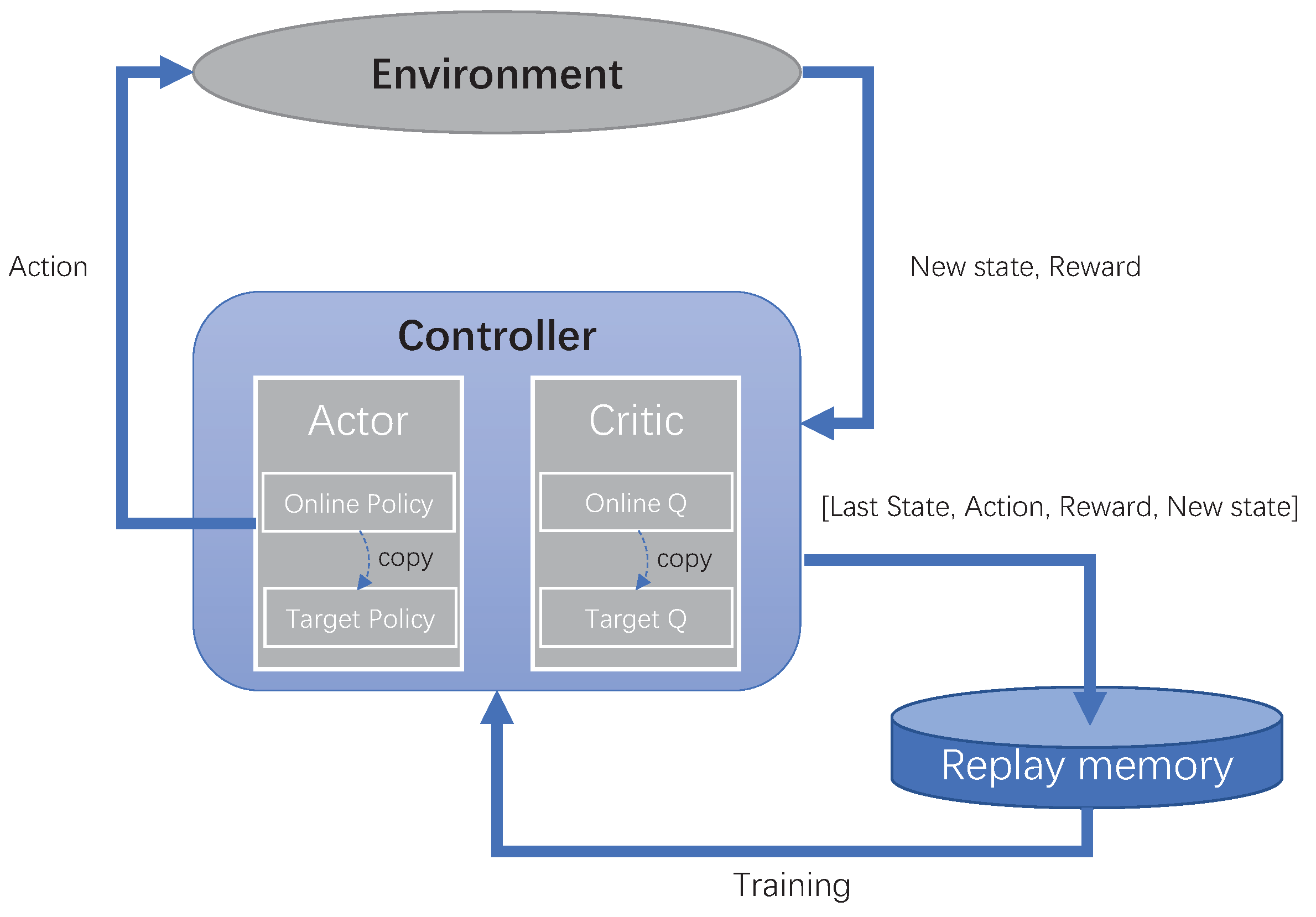
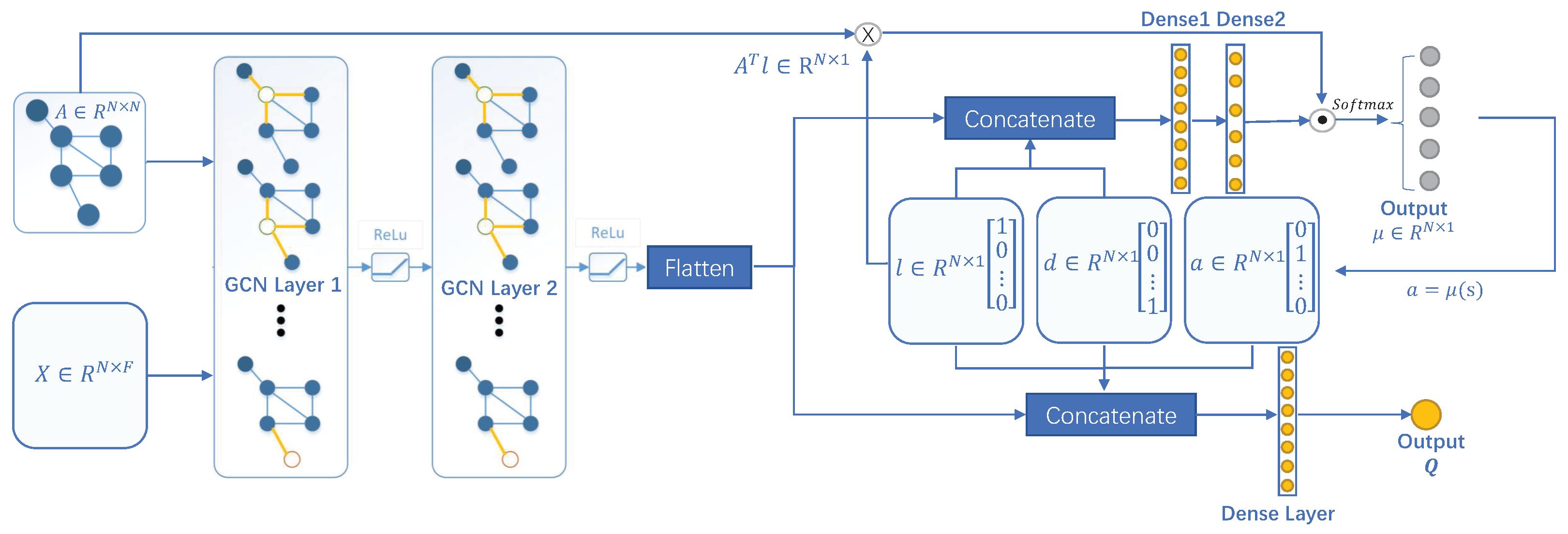
  • We designed an actor–critic network architecture for the DRGL model, which takes into account both graph convolutional networks and deterministic policy gradient. Reward functions for the reinforcement learning and training method were developed for the DRGL model.
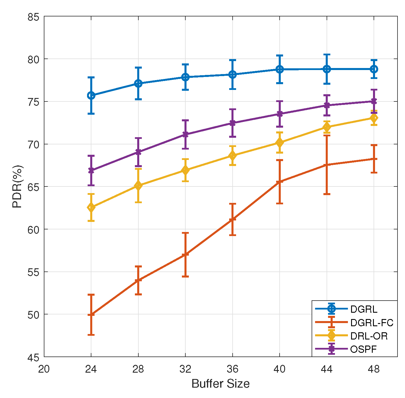
  • Compared with traditional routing protocols, the proposed DGRL traffic control mechanism can effectively reduce the probability of network congestion, especially in the case of high concurrent traffic intensity. Simulation experiments based on the Omnet++ platform show that, compared with existing traffic routing algorithms for SDWSNs, the proposed intelligent routing control method can effectively reduce packet transmission delay, increase PDR (Packet Delivery Ratio), and reduce the probability of network congestion.
The rest of the paper is organized as follows. Section 2 summarizes the related literature in the research direction. Section 3 describes the system structure of the proposed deep reinforcement learning model DGRL in detail. We also discuss the specific training method and updating process when the simulation network is running. Section 4 shows detailed experimental results and presents performance evaluation. Section 5 presents discussion and challenges associated with DGRL. Section 6 concludes the paper and discusses future work.

2. Related Works

Several researches use traditional methods for intelligent routing control. Literature [10] introduces a node mobility prediction scheme to enhance the network throughput. The controller predicts node mobility through machine learning and sends optimal route information to the data plane in preparation for upcoming link failures. In the literature [11], a control mechanism based on context-driven is introduced in the scenario of SDN. It contributes to improving the autonomous capability of the network. In the literature [12], a hybrid network search path scheme is designed for intelligent traffic forwarding. Dijkstra and K path forwarding algorithm are used under different network loads. Literature [13] introduces a probabilistic-based QoS routing mechanism for SDN to reduce bandwidth blocking. Bayes’ theorem and the Bayesian network model are used to determine the link probability and select the route.
Artificial neural network extracts features data by imitating the way that neurons processes the input information. It is the main means of intelligent information processing nowadays. With the increase of GPU computing power, end-to-end models based on deep learning have become state-of-the-art in the fields of computer vision, natural language processing, and reinforcement learning [14].
The application of deep learning and reinforcement learning to network traffic control and routing forwarding is a relatively new application scenario which has received a lot of attention in recent years. Tang et al. [15] introduce the deep convolutional neural network into the Wireless Mesh Network (WMN). The traffic pattern of sensor network is sent to the deep neural network in the form of multi-channel tensor for training, and the optimal routing strategy is obtained. In the literature [16], the author tries to replace the original routing strategy by training multiple restricted Boltzmann machines. Correspondingly, this can effectively reduce the data transmission delay and improve the overall transmission efficiency. However, this method is only suitable for small sensor networks. Once the number of nodes increases, the number of neural networks to be trained will also increase exponentially. In our previous work [17], we study the combination of deep learning and WSN with super nodes. Through link reliability prediction, the routing decision algorithm is introduced to reduce the overall transmission delay and effectively improve the network life. Literature [18] combines convolutional neural network with restricted Boltzmann machines to calculate routing for software-defined routers in wireless mesh sensor networks. Literature [19] uses the three-dimensional tensor formed by the time series traffic patterns of nodes in the network for training. It also explores the influence of the deep model and the shallow model on the training effect. Deep learning is also used in scenarios such as intelligent channel allocation and traffic prediction [18,20]. Due to the characteristics of data transmission policy for software-defined sensor network, offline algorithms such as deep learning cannot match the dynamic characteristics of network data forwarding.
In [21,22], conversion of traditional routing rules into computational paradigms is investigated based on deep learning and reinforcement learning respectively. Younus et al. [8] introduce reinforcement learning into the software-defined wireless sensor network. By designing a quadruple reward function and combining with the Q-Learning algorithm [23], it effectively improves the energy efficiency of the SDWSN and prolongs the lifetime of network nodes. Some routing planning algorithms are proposed based on Q-Learning, such as the QELAR model proposed by Hu et al. [24], the SDWSN model proposed by Huang et al. [25], and the DACR routing algorithm proposed by Razzaque et al. [26]. These models are designed to improve the energy efficiency of nodes and the quality of service (QoS) of WSN. Deterministic policy gradient (DPG) [27] applies to routing policy in continuous action space, while Q-Learning applies to finite state space in specific scenarios. Deep deterministic policy gradient (DDPG) [28] and deep Q network (DQN) [29] are the products of the combination of deep learning and reinforcement learning, which effectively improves the feature expression ability and decision-making ability of reinforcement learning. Liu et al. [30] simultaneously introduced DQN and DDPG into routing policy, which greatly improves the throughput of the network and made the network load more balanced. Their experimental results show that DDPG has a better decision-making effect than DQN in continuous state space. Yu et al. [31] generated a routing policy by using DDPG to predict node connection weights. The network transmission delay is therefore reduced. Abbasloo et al. [32] proposed the Orca model, which effectively solves the congestion control requirements of the TCP protocol of the transport layer. By integrating the deep policy gradient algorithm, they introduced the congestion window and the network data forwarding pacing rate. Due to the black box characteristics of deep reinforcement learning, Meng et al. [33] proposed the Metis framework. By introducing two different interpretation methods based on decision trees and hypergraphs, the DNN policy is transformed into an interpretable rule-based controller. To a certain extent, it demonstrates the feasibility of using deep reinforcement learning for network traffic control.
We compare the literatures using reinforcement learning mentioned above and summarize them in Table 1.

3. System Design

In this section we describe the design of DGRL, a distributed traffic control algorithm model based on deep graph reinforcement learning. The model DGRL uses an experience pool for playback training. Each node in the model can optimize its own transmission path through online training and make the best next-hop policy. It is a lightweight and real-time routing control algorithm for data forwarding.

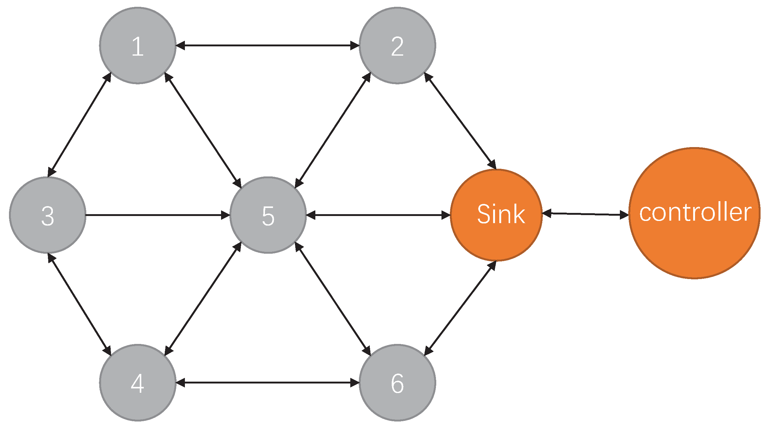
3.1. Problem Statement and Notations

A SDN-based WSN is represented by a topology adjacency matrix A. We assume that the controller can receive timely updates of the network state S (e.g., channel delay, loss rate, and buffer occupancy of nodes). The controller generates a policy μ for the nodes to forward packets. The policy determines routing paths based on the network state: a t = μ ( S t | θ μ ) . The reward for taking action a t in state S t can be represent by R μ ( a t , S t ) . The performance of policy μ will be measured by function Q ( μ ) . The problem is defined as follows. Given A, S, find a policy to determine the path for forwarding packets. Our goal is to find the optimal behavior policy μ , which is to maximize the function Q ( μ ) : μ = a r g m a x μ Q ( μ ) .
Table 2 summarizes the important notations used in DGRL.

3.2. System Framework of DGRL

The system block diagram of the controller is shown in Figure 2. The E n v i r o n m e n t represents the network to which the controller is connected. The controller captures the current network status from the environment and uses the O n l i n e P o l i c y in the Actor neural network to make policy. The previous state, action made by the controller, reward value of the environment feedback, and the latest observed SDN state form a four-tuple record ( L a s t S t a t e , A c t i o n , R e w a r d , N e w S t a t e ). The four-tuple is stored in the experience pool for training multiple neural network models. One is the O n l i n e Q in Critic NN, and the other is the decision network O n l i n e P o l i c y in Actor NN. The O n l i n e P o l i c y is used to make decisions μ based on the state of the current environment: state → action, while the O n l i n e Q is used to fit the reward of the environment for the controller’s decision: (state, action) → reward. Both the O n l i n e P o l i c y and the O n l i n e Q have exactly the same target network as their structure, named T a r g e t P o l i c y and T a r g e t Q , respectively. The purpose is to use soft updates to assist the training process to achieve convergence and avoid large gradient fluctuations during training.
In general, the Actor NN and Critic NN both contain two parts, namely online network and target network. O n l i n e P o l i c y outputs real-time actions for the Actor NN to use in real time. The T a r g e t P o l i c y is used to update the Critic NN. The output of O n l i n e Q and T a r g e t Q are both the value of one state, while the input is different. O n l i n e Q takes the actual actions taken by the Actor NN and the current state as input. T a r g e t Q uses the output of T a r g e t p o l i c y . Details about the feedforward processes for the Actor NN and the Critic NN can be found in Section 3.3.
The structure diagram of the Actor neural network and Critic neural network is shown in Figure 3. Actor neural network is at the top of the figure, and Critic neural network is at the bottom of the figure. The blue rectangles in Figure 3 represent tensor transformation operations, the golden circles represent neurons, and the gray circles represent tensors. The Actor model contains four inputs, topological adjacency matrix A of the network, current features X of all nodes, one-hot code l of the node where the data packet is currently located, and one-hot code d of the destination node. The state of the current node and the state of neighbors must be considered when transmitting data packets. Actor uses graph convolutional neural network to extract and aggregate the state features of the current node and all its neighbors. Since it is highly correlated with data forwarding, the destination node is necessary to be considered after extracting the network state. Therefore, we flatten the output of the GCN layers and concatenate the result with l , d . The vector s t a t e represents the state features of the network environment, which is given by
s t a t e = [ F l a t t e n ( G C N ( A , G C N ( A , X ) ) d l ]
where G C N represents the graph convolution operation, ‖ means concatenate. The detailed calculation of GCN will be given in the next subsection.
The output μ of the Actor model is generated by Hadamard product operation which consists of the result of fully connected layers and an inner product operation. The activation function of this layer is Softmax, and the output is the next hop policy μ of the current data packet.
The Critic model contains five inputs. In addition to the four input parameters for the Actor model, it also includes the next hop action a obtained by the Actor model. The Critic model also contains the GCN layers for extracting the characteristics of the controller and its neighbor nodes, but the weights of the GCN layers are not trainable. Its weights are completely copied from the corresponding GCN layers of the Actor model. The purpose is to ensure that the state features of all nodes extracted by the two model are completely consistent. The Critic model contains a connected layer. The outermost layer uses a single neuron to fit the feedback value Q of the action policy adopted by the model.

3.3. Feedforward Processes for Actor and Critic Models

3.3.1. Feedforward Calculation of Actor Neural Network

First, we give the feedforward process of the graph convolutional layer. We use A i , j and X to denote the topological adjacency matrix of the sensor network and the state of network observed by the controller, respectively. The number of nodes and the number of features are denoted by N and F, respectively. Apparently, we have A i , j R N × N and X R N × F . We define an adjacency matrix with self-loop A ^ i , j = I N + A i , j , where I N is the unit matrix of order N. Thus, the degree matrix D i , j R N × N is
D i , j = j A ^ i , j i f i = j 0 e l s e
In the process of graph convolution calculation, nodes with too many neighbor nodes will have a large gap with other nodes when aggregating features. To avoid this problem, we define the standardized adjacency matrix as A ˜ i , j = D i , j 1 / 2 A ˜ i , j D i , j 1 / 2 . After two graph convolutional layers, the output tensor H is obtained by
H = R e L U ( A ˜ i , j ( R e L U ( A ˜ i , j X W g ( 0 ) + b g ( 0 ) ) ) W g ( 1 ) + b g ( 1 ) )
where W g ( 0 ) R F × C , b g ( 0 ) R C × 1 , W g ( 1 ) R C × Z , b g ( 1 ) R Z × 1 are the weights that need to be trained in the Actor model. C and Z are the characteristic dimensions of the output after graph convolution.
In addition to the adjacency matrix A i , j and the state matrix X, the Actor model also includes the position vector l R N × 1 of the current node and the vector d R N × 1 of the target node. Both vectors are composed of one-hot codes, which represents the unique ID of nodes.
The state vector of the current environment S can be obtained by
S = C o n c a t e n a t e ( F l a t t e n ( H ) , l , d )
In (4), the dimension of S is N × Z + 2 N .
The state vector S will be used as the input of the fully connected neural network in the Actor model, and finally the corresponding action vector μ R N × 1 is obtained at the output of the Actor. This vector determines the next hop after the current node receives the data packet. Since the network topology is not fully connected in most cases, it is necessary to use the mask vector to filter the action vector output by the Actor fully connected layer. The vector m a s k represents the adjacency information of the node where the packet is located. It can be calculated by
m a s k = A i , j T l
where A i , j T is the transpose of the adjacency matrix. Specifically, the purpose of setting the mask vector is to limit the decision space and avoid forwarding data packets to non-neighbor nodes.
The final output of the Actor model can be obtained by
μ = s o f t m a x ( m a s k ( W a S + b a ) )
where ⨀ represents the Hadamard product, and W a , b a are the weights of the fully connected layer.

3.3.2. Feedforward Calculation of Critic Neural Network

It has been mentioned in the last section that the weights of the GCN layers in the Critic model are completely replicated from the Actor network. The feedforward calculation process and results of the GCN layers are completely consistent with that in the Actor model, and this section will not repeat it again. After obtaining the output μ of the Actor model, we define a = μ + N t , where N t is a random disturbance term. Next, we can obtain the output y of the Critic model by the following equation:
y = L i n e a r ( W C ( 1 ) R e L U ( W c ( 0 ) [ S a ] + b c ( 0 ) ) + b c ( 1 ) ) )
where ‖ represents a concatenate operation, S is the tensor output by GCN, W c ( i ) , b c ( i ) are the weights of the i-th fully connected layer.

3.4. Design of DGRL Training Method, Controller Node Features and Reward Function

3.4.1. The Training Method of DGRL

The model proposed in this paper is based on the deterministic policy gradient and this framework is based on Q-value. The Critic neural network of DGRL is used for Q-Value fitting. The quality of the policy can be expressed by the expected value according to the following equation:
Q ( S t , a t ) = E K γ k R ( S t + k , a t + k )
where R t = R ( S t , a t ) is the feedback value of the environment, and γ is the time series decrement factor.
Taking t = 2 as an example, the iterative formula of Q ( S 2 , a 2 ) can be obtained by approximating Equation (8) as follows:
Q ( S 2 , a 2 ) = E R 2 + γ R 3 + + γ n 2 R n = E R 2 + E γ R 3 + + γ n 2 R n R 2 + E γ R 3 + + γ n 2 R n R 2 + γ Q ( S 3 , a 3 )
Inductive Equation (9) can get the iterative formula as shown in (10):
Q ( S t , a t ) = E R t + γ Q ( S t + 1 , a t + 1 ) R t + γ Q ( S t + 1 , a t + 1 )
Define y t = R t + γ Q * ( S t + 1 , a t + 1 * ) , where a t + 1 * is the output of the T a r g e t P o l i c y and Q * ( S t + 1 , a t + 1 * ) is the output of the T a r g e t Q . Then the loss function of the O n l i n e Q can be defined as follows:
L ( θ Q ) = 1 N t ( Q ( S t , a t ) y t ) 2 = 1 N t ( Q ( S t , a t ) ( R t + γ Q * ( S t + 1 , a t + 1 ) ) ) 2
where θ Q is all the weights that need to be trained in the O n l i n e Q model, Q ( S t , a t ) is the output of the O n l i n e Q model, and n is the batch size. At this point, replay can be done by sampling the four tuples (Last State, Action, Reward, New State) in the experience pool of DGRL model. The error back-propagation algorithm can be used to train the O n l i n e Q network and update all its internal weights θ Q .
All weights of the O n l i n e P o l i c y are represented by θ μ . Its update is slightly different from the Critic network because O n l i n e P o l i c y does not have explicit label data. However, through the deterministic gradient policy, it can be known that a good policy will get a larger Q value. Given the gradient of the loss function for Critic network and the output policy μ ( S t ) of the O n l i n e P o l i c y , the weight gradient update of the Q value can be obtained as follows:
θ μ L = 1 n t a Q ( S t , a t θ Q ) θ μ μ ( S t θ μ )
Where a t = μ ( S t θ μ ) + N t , N t is an Ornstein–Uhlenbeck stochastic process with 0 mean characteristics [34]. It enables the agent to explore beyond the learned policy, and avoids the network from falling into a local optimal policy.
The initial weights of the T a r g e t Q model and the T a r g e t P o l i c y model θ Q * , θ μ * are completely copied from the respective corresponding models: θ Q * θ Q ; θ μ * θ μ . After the weights of the Critic and Actor models have been updated through training, the Target model uses a soft update to update the weights, as shown in Equation (13). A soft update is used to assist the training process to reach the convergence state.
θ Q * = τ θ Q + ( 1 τ ) θ Q * θ μ * = τ θ μ + ( 1 τ ) θ μ *

3.4.2. Design of Node Characteristics and Reward Function

In the process of deep reinforcement learning, the controller needs to observe the state of the system to obtain the feedback after executing the forwarding policy. In this paper, the state matrix X t R N × F is composed of four features of all nodes, which are: number of connections per node, average transmission delay of the channel (link quality), packet loss rate of nodes, and occupancy of node buffer.
The designed objective function can guide the controller to forward the data packet towards a high benefit goal. High benefit is defined as: shorter forwarding time, shorter forwarding path, lower buffer occupation. In this paper, the reward function is as follows:
R ( t ) = 1 d e l a y p r e × d i s t a n c e × b u f f e r + 1
where d e l a y p r e represents the time taken by the data packet from the previous node to the current node and d i s t a n c e [ 0 , 1 ] represents the relative distance of the data packet to its destination node. The relative distance is calculated by the ratio of the total hops of the shortest path from the packet to its destination to the total number of nodes (in a weighted network, the sum of the shortest path weights and the weights of all edges is calculated). b u f f e r ( 0 , 1 ] represents the occupancy of the node buffer after receiving the data packet. The buffer of each node stores the data packets to be sent, and the occupation of buffer determines the packet loss and congestion of the network. The reason for using these three items is to avoid the larger order of magnitude factor from occupying a dominant position in the optimization process. Therefore, the three objectives will be optimized at the same time. The design of R ( t ) ensures that R ( t ) [ 0 , 1 ] , which is equivalent to a standardized operation and beneficial to the training of deep neural network. It is important to note that when the data packet has reached the destination node, d i s t a n c e = 0 , R ( t ) = 1 ; when the data packet is discarded because the buffer queue is full or TTL (Time to Live) arrives, set R ( t ) = 0 .

3.5. Traffic Control Based on Deep Graph Reinforcement Learning

The traffic control model based on deep graph reinforcement learning includes two phases. One is the data collection stage when the simulation network is running, and the other is the training stage. When the network is running, each node following the policy forwarded by the controller determines the next hop according to the current state of the WSN. After the forwarding task is performed, the next hop node will integrate the real-time state and reward value into a four-tuple record ( L a s t S t a t e , A c t i o n , R e w a r d , N e w S t a t e ), and store it in the experience pool for training. For a detailed process description, see Algorithms 1 and 2.
Algorithm 1 Running phase
Input: batch size, θ μ *
Load the weights: θ μ * for target Actor model
 1:
Generating data packet p, using θ μ * and stochastic OU process to determine its next hop a, and recording it together with the current network state. p : = d e s t i n a t i o n , l o c a t i o n , s t a t e , a , d a t a
 2:
while L e n g t h ( E x p e r i e n c e R e p l a y ) < b a t c h s i z e do
 3:
    if packet p received then
 4:
        if p has arrived at its destination then
 5:
           done=True
 6:
        else
 7:
           done=False
 8:
        end if
 9:
        observe the network to get the new state, calculate the reward r for p a and
 9:
         append experience replay list with p s t a t e , p a , r , n e w s t a t e , d o n e
 10:
         p s t a t e : = n e w s t a t e ; p l o c a t i o n : = l o c a t i o n
 11:
        if not done then
 12:
           use θ μ * to determine its next hop a
 13:
            p a : = a
 14:
           send data packet p
 15:
        end if
 16:
    end if
 17:
end while
It should be noted in the Running Phase that θ μ * is obtained by the shortest path method if the deep reinforcement learning neural network model has not yet started training. After collecting enough data, the Training Phase will start. The weights of all the deep graph neural networks in the model will be updated by experience playback and gradient descent. After the training, each node will use the updated weights to choose a better next hop for the packets in the Running Phase.
Algorithm 2 Training phase
Input: Adjacency matrix A of the SDN, Experience Replay, τ
 1:
if Training phase is running for the 1st time then
 2:
    randomly initialize Actor model θ μ and Critic model θ Q , with target Critic model θ Q * : = θ Q and target Actor model θ μ * : = θ μ
 3:
else
 4:
    load weights θ Q * and θ μ * from the disk, with θ Q : = θ Q * and θ μ : = θ μ *
 5:
end if
 6:
for each s t a t e , a , r , n e w s t a t e in Experience Replay do
 7:
     a = θ μ * ( s t a t e )
 8:
     y = r + γ θ Q * ( n e w s t a t e , a )
 9:
     L ( θ Q ) = ( y θ Q ( s t a t e , a ) ) 2
 10:
    Use L ( θ Q ) to update the weights of θ Q using gradient descent
 11:
    Use a L ( θ Q ) θ μ μ ( s t a t e θ μ ) to update the weights of θ μ
 12:
    update target model θ Q * and θ μ * :
 12:
                      θ Q * : = τ θ Q + ( 1 τ ) θ Q *
 12:
                      θ μ * : = τ θ μ + ( 1 τ ) θ μ *
 13:
end for
 14:
save weights θ Q * , θ μ * on the disk respectively.
The weights of Policy network θ μ updated in the Training Phase will be stored and used for the packet forwarding in the Running Phase. At the same time, weights of Target Q model θ Q * and weights of Target Policy model θ μ * will be stored and used as the initial value for the next training phase.
After many iterations of data collection and training, the controller will become smart enough to make the best next hop policy for all packets passing through the node at the packet-level. The policy considers the transmission delay, buffer occupancy, and the distance from the destination node at the same time. The data forwarding and traffic control policy based on deep graph reinforcement learning mentioned in this paper can be trained online by combining two phases, and the O n l i n e P o l i c y deep neural network used for decision-making can be updated in real time.

4. Evaluation

In this section, we focus on evaluating our approach’s performance in different traffic intensity and comparing it with some related algorithms. We first describe our simulation parameters, simulation environment, and evaluation metrics. Then, we train the model and evaluate its performance based on a series of experiments.

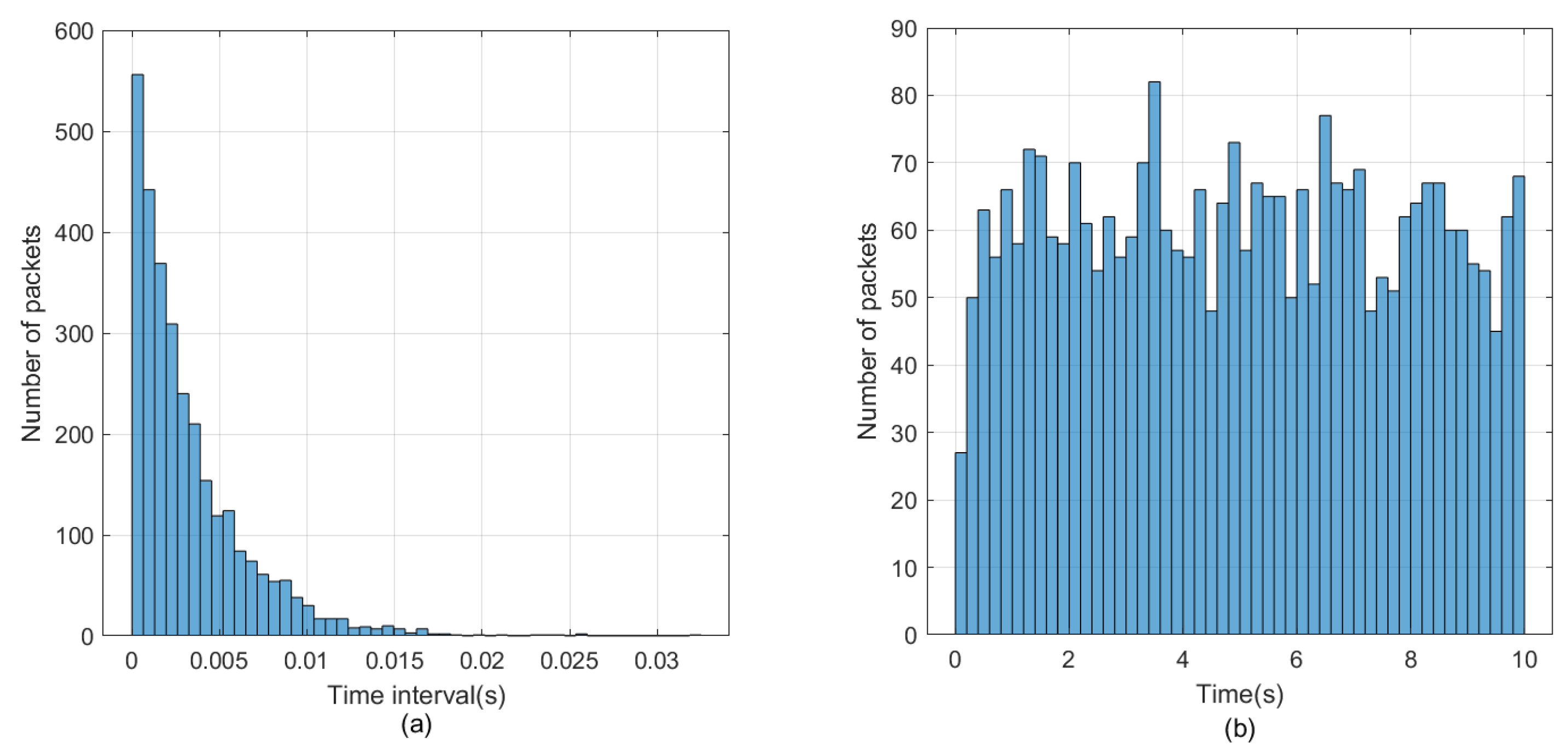
4.1. Simulation Environment

4.1.1. Operation Platform

The simulation part is completed by OMNET++4.6.0, and the deep learning model of DGRL is built by TENSORFLOW 1.14.0 with the following experimental environment: Intel(R) Core(TM) i5-8300H, 16G RAM, NVIDIA GeForce GTX 2060.

4.1.2. Parameter Setting

Table 3 shows the parameter settings of network. We perform an evaluation of some hyperparameters of the DGRL implentation to optimize the performance of the agent, specifically for our problem environment. Particulary, we consider the following three hyperparameters: the ratio of soft replacement T A U , learning rate for the Actor model a _ l r and learning rate for critic model c _ l r . Figure 4 presents the results of this evaluation. The settings for these three hyperparameters and some others can be found in Table 4. Table 5 gives the details of the Actor model and the Critic model.

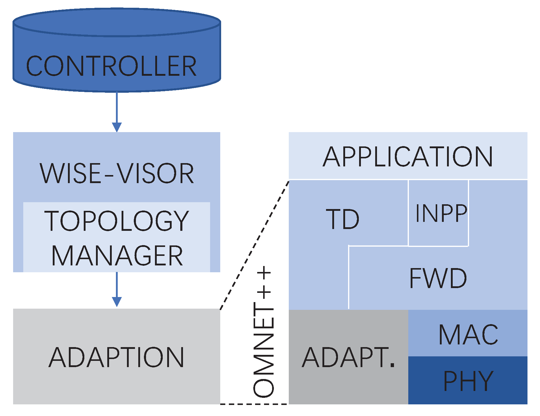
4.1.3. Protocol Architecture

The protocol architecture of DGRL is shown in Figure 5. Network logics are dictated by controller and wise-visor. The adaption layer between the wise-visor and nodes is responsible for formatting messages received from nodes in such a way that they can be handled by the wise-visor, and vice versa. On top of the mac layer, the forwarding (FWD) layer handles incoming packets as specified in the flow table. The FWD layer updates the flow table according to the configurations sent by the control plane. The In-Network Packet Processing (INPP) layer runs on top of the forwarding layer and it is responsible for operations like data aggregation or other in-network processing. Topology discovery (TD) layer uses beacon packets to help nodes discover their interconnected nodes. This part of the protocol structure is set according to the literature [4].

4.2. Compared Algorithm Models

1.
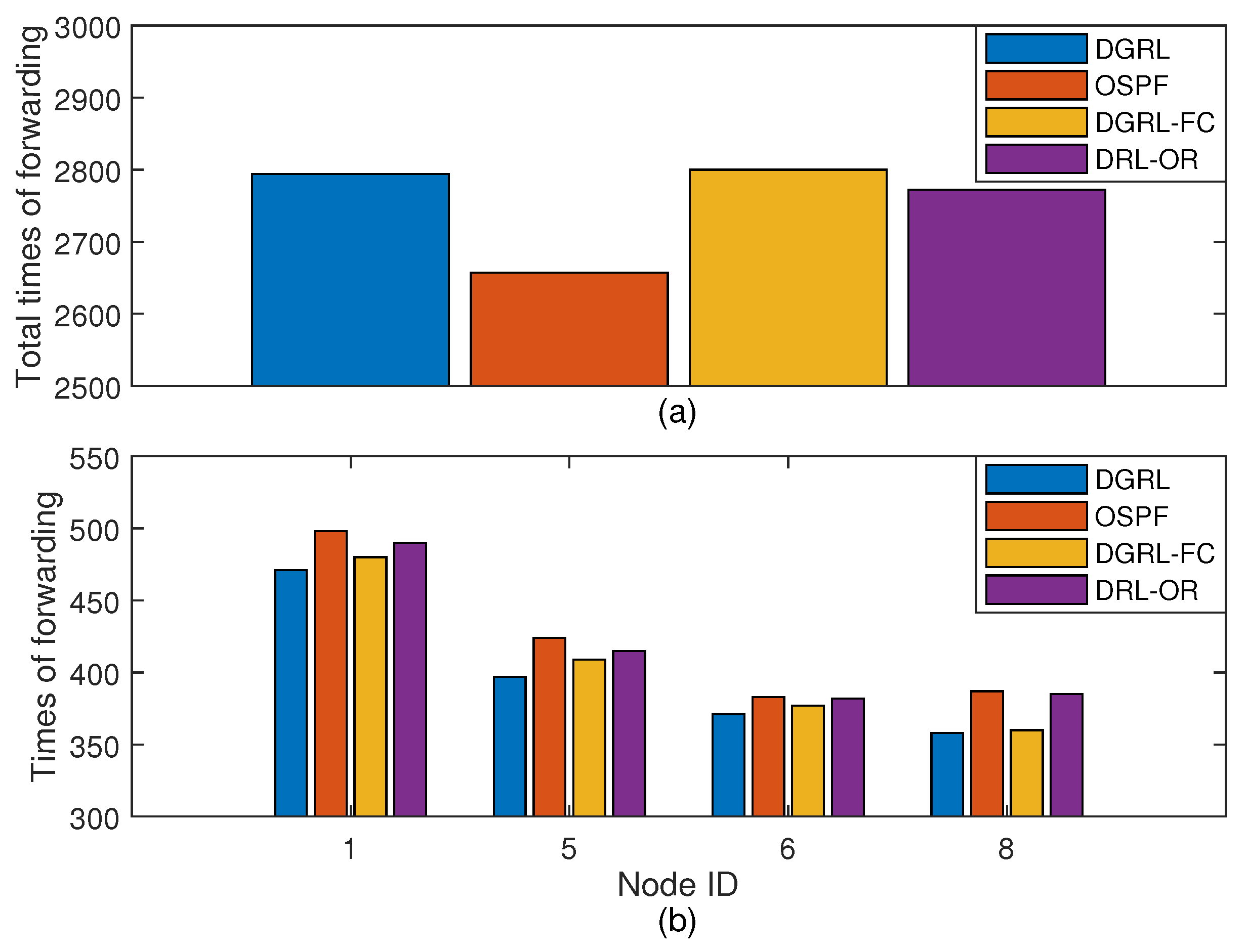
Open Shortest Path First (OSPF): According to the directed graph of the network topology, the algorithm generates a shortest path tree as a static routing table. Nodes will forward packets based on the flow table generated by this static routing table.
2.
Deep Reinforcement Learning-Optimized Routing (DRL-OR) [35]: The model contains two fully connected layers and uses the traffic features of nodes to represent the network state. The dimension of state is 182. Its Actor and Critical models are two-layer perceptron structures, and the dimensions of perceptron are [91,42].
3.
Deep Reinforcement Learning-Full Connect (DGRL-FC): All GCN layers of the proposed DGRL model are removed, and only the perceptron layers of each model are retained. The other neural network parameters are completely consistent with DGRL.

4.3. Performance Evaluation Metrics

In the process of experiment, the related metrics are obtained by OMNeT++ including packet loss rate, average delay, and total number of packets forwarded. The notations involved in the following calculation formulas are explained in Table 1.

4.3.1. Average Network Delay
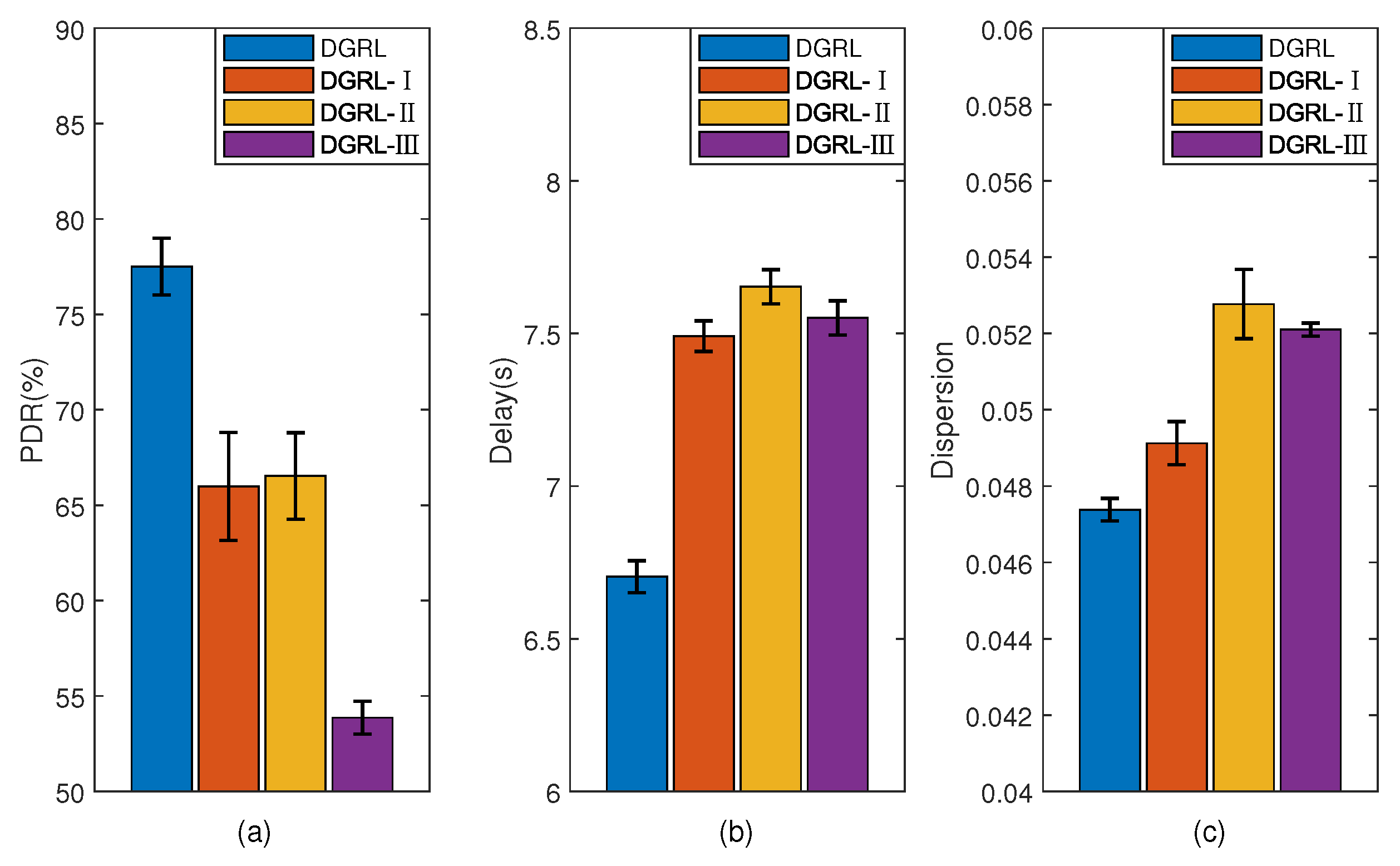
D e l a y refers to the average transmission time of all packets reaching the destination nodes.
D e l a y = j = 0 J 1 T r j T s j i = 0 N 1 P r n i

4.3.2. PDR

P D R represents the ratio between packets received by the destination nodes and packets sent by the source nodes. This metric reflects the adaptability of solution under different traffic intensity.
P D R = i = 0 N 1 P r n i i = 0 N 1 P r n i + P d n i

4.3.3. Dispersion of Routing Load
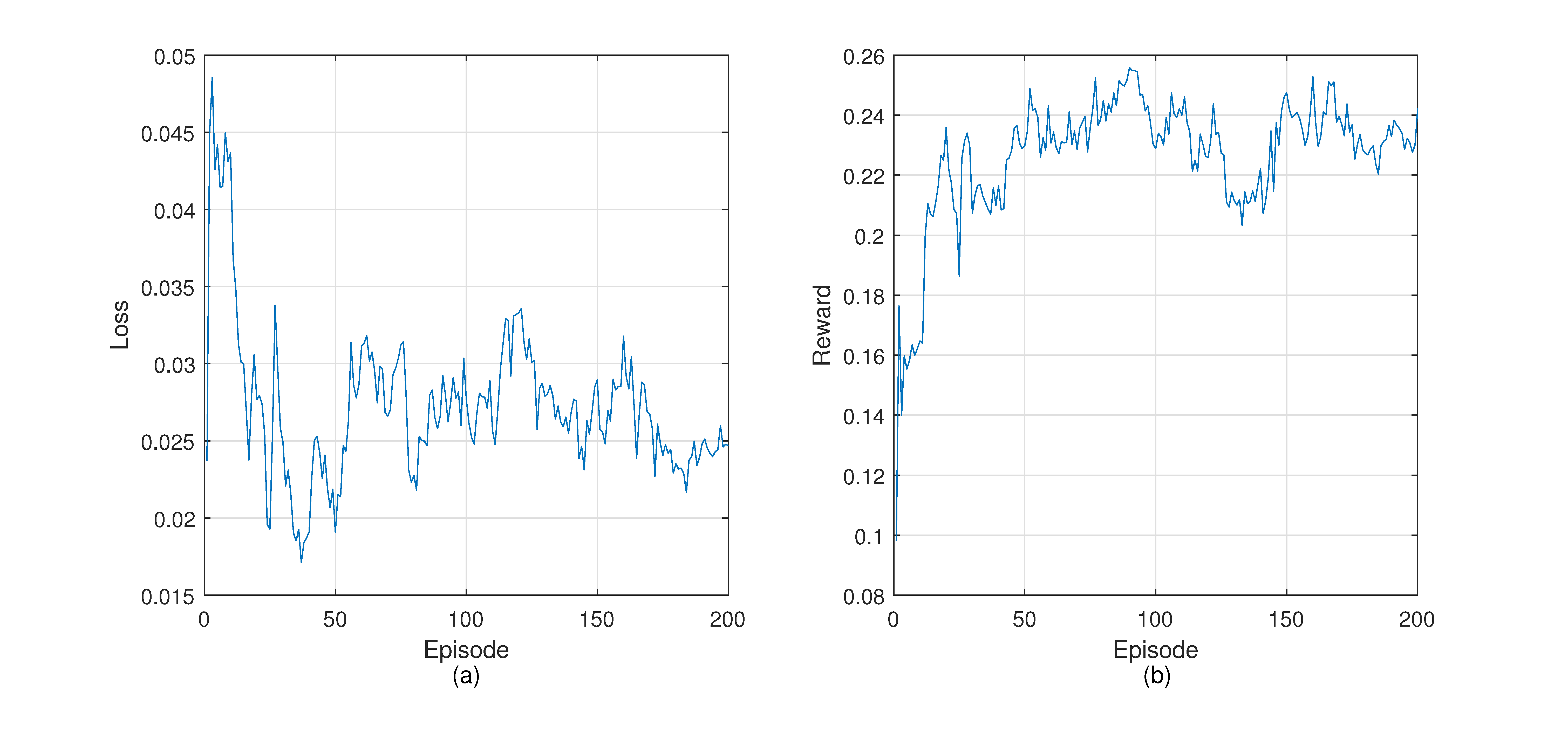
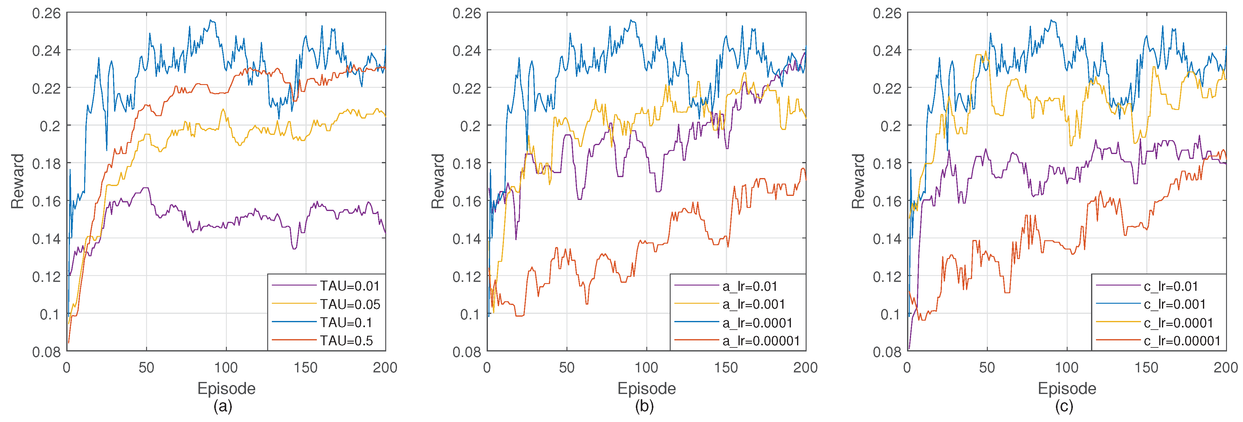
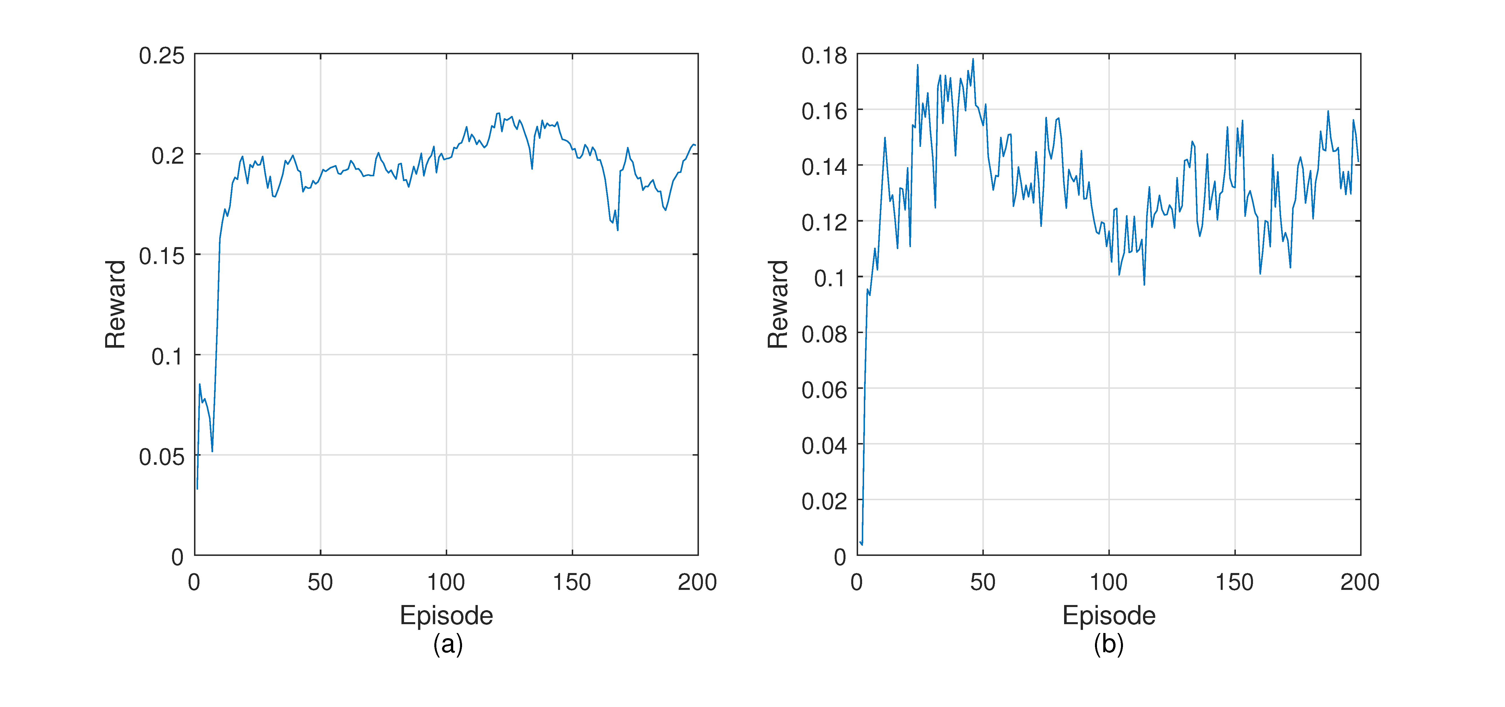
Dispersion of routing load indicates the evenness of load distribution in a network. A large dispersion indicates that the load in the network is not balanced. A relatively single and fixed route will produce this result, which will lead to congestion at nodes and even network crash.
D i s p e r s i o n = i = 0 N β i β ¯ 2 N

4.4. Training DGRL

For training purpose, we built six traffic intensity models ranging from 20% to 125%. The traffic intensity is reflected as the time interval between packet generation. Figure 6 shows the traffic model when the traffic intensity is 125%. Figure 6a shows the time interval distribution of data packets, and Figure 6b shows the number of data packets sent.
The shortest path algorithm Dijkstra is used to generate the initial packet transmission path, as well as the relevant environment data, including channel delay, packet loss rate of nodes, the occupancy of buffers, and the generated rewards value.
After the pre-training, the model is used to predict the transmission direction in the simulation environment. We will collect the environment data and the corresponding reward value and store them in the experience pool. The weights of all the neural networks in the model will be updated by experience playback and gradient descent. The loop will be repeated 200 times, each of which comprises 100 steps.
Figure 7 shows the loss and reward during the training process. The loss curve shows a downward trend on the whole. However, the loss often increases throughout the training. This can be explained by the difference between reinforcement learning and supervised learning based on fixed data sets. The training data of reinforcement learning come from the experience pool, and the data in the experience pool are collected from the environment, so they are in constant change. The loss curve fluctuates when encountering a new state space that leads to better reward. In the beginning, the reward is lower because the controller does not have enough knowledge about the network and explores the environment. After some training episodes, the reward increases rapidly. It reflects that routing policies made by the controller are able to guide packets forwarding to obtain better returns.

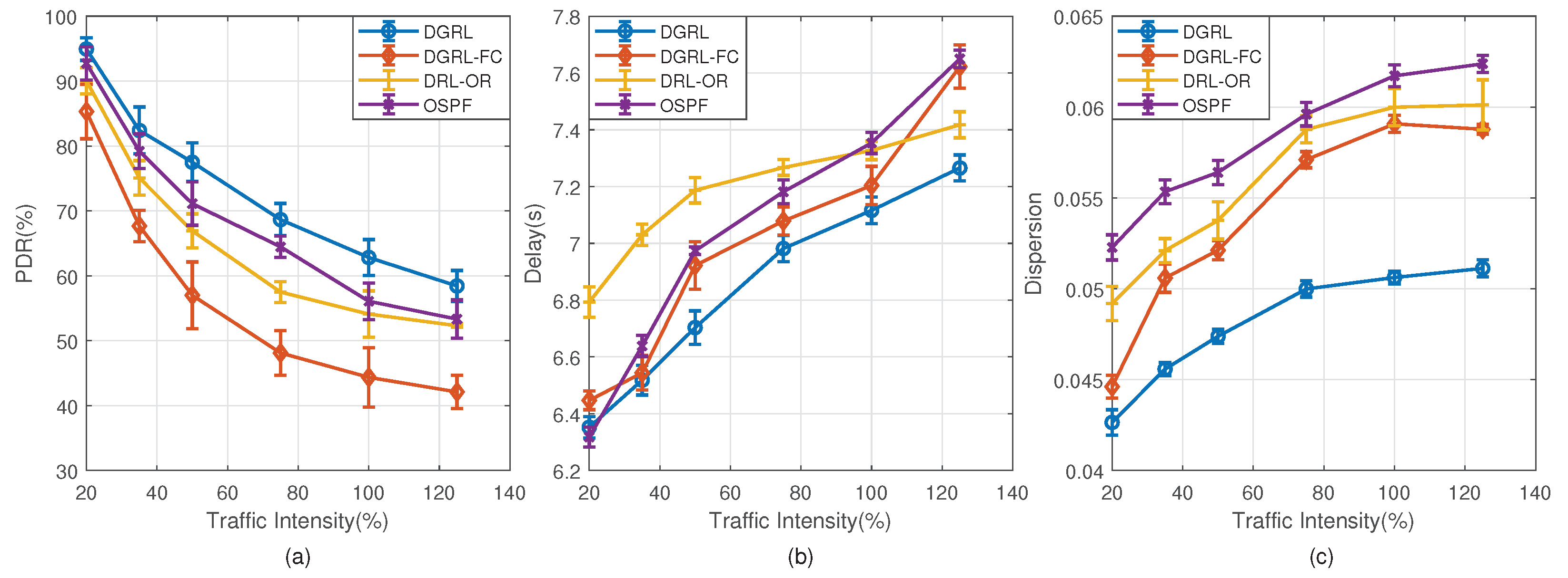
4.5. Evaluation Results

Figure 8 reflects the performance of DGRL and the three comparison algorithms under different traffic intensity. The numbers on the x-axis are the number of traffic intensity, while the numbers on the y-axis are the number of PDR, transmission delay, and load dispersion, respectively.
Figure 8a describes the packet delivery rate. For limited buffer, the increase of traffic intensity is prone to packet loss, which reduces the delivery rate and makes the network difficult to operate properly. Reinforcement learning helps DGRL select better routes and increase packet arrival through environmental data. As you can see from Figure 8a, DGRL has a better delivery rate than other algorithms. Under the traffic intensity 125%, the PDR of DGRL is 5.1% higher than OSPF on average. The performance of DRL-OR is close to OSPF. From traffic intensity 75%, the PDR of DGRL-FC is less than 50%, while we notice that the PDR of others can be maintained above 50%.
Figure 8b shows the average transmission delay for four different algorithms. Each port of each node has a buffer of length 32. If the channel is free, the packets will be sent out immediately. Otherwise, they will be stored in the buffer and queue for being sent out. In this experiment, the transmission delay of data packets mainly comes from the time they queue for forwarding in the node buffer. Under low traffic intensity, the average delay of each algorithm is similar. That is because the buffers are still free, and the waiting time required for forwarding is also short. When the traffic intensity increases, the buffer occupancy rises and even the buffers are filled up. In this case, more time will be spent through this node and even packet loss will occur. OSPF considers only the shortest path, so the forwarding path is fixed. Based on the smallest number of hops, the forwarding is efficient at low traffic intensity. Under the traffic intensity 20%, it has the best performance compared with other algorithms. From traffic intensity 100%, its delay turns out to be the worst. DGRL-FC is similar to DGRL in that it considers the features of nodes, but it lacks consideration of the relationship between nodes and its neighbors. In the case of high traffic intensity, the optimization effect is poor. DRL-OR takes the traffic characteristics into consideration, alleviates congestion, and reduces delay to a certain extent. However, its delay is higher than others when the traffic intensity is low. Different from other algorithms, DGRL considers multiple factors in routing decisions, including hops and buffer occupancy. It is able to adjust the forwarding route flexibly. Under low traffic intensity, it forwards packets according to the hops. When the traffic intensity increases, buffer occupancy will play a more critical role in routing decisions.
Figure 8c shows the dispersion of network load. In this experiment, the source and destination nodes of data packets are both random. Therefore, the difference of network load dispersion comes from routing. It is apparent that the network using DGRL has the smallest dispersion, while the network using OSPF has the largest dispersion. For example, under the traffic intensity 125%, the dispersion of load in network using DGRL is 0.051, whereas those of OSPF, DRL-OC, and DGRL-FC are 0.062, 0.060, and 0.058, respectively. These results confirm DGRL’s effectiveness in adjusting network load. The reasons behind lower dispersion are as follows. DGRL is an algorithm with memory. It will learn from the experience. Suppose that in a state s, the action a forwards the packet to a next hop whose buffer occupancy is high. The reward of this action will be low. When it is in the state s again, it remembers that a contributes to a higher reward than a. Therefore, it avoids forwarding packets to high occupancy nodes. In the model using OSPF, some nodes are on the shortest path of multiple source-destination nodes pairs. These nodes will bear more forwarding than edge nodes. The situation is more serious with the increase of traffic intensity.
In our experiments, the new received packets will be dropped when the buffer is full. PDR is the most direct index to reflect packet loss. We designed a new experiment to verify the relationship between PDR and buffer size. The traffic intensity is fixed at 50% and the buffer size ranges from 24 to 48. Figure 9 shows the PDR curves of each model. As we can see from the figure, buffer size has little effect on DGRL. When the buffer size is 32, as set in the previous experiments, the PDR of DGRL is 77.9%. When the buffer size is reduced to 28 and 24, the PDR decreased by 0.7% and 1.4%, respectively. When the buffer size increases to 48, the increase of PDR is little. This can be understood as DGRL has a better utilization rate for the network buffers. A buffer of size 32 already meets the requirements of DGRL. The PDR of the other three models are closely related to buffer size. As buffer size decreases from 32 to 24, the PDR of OSPF decreases by 4.2%, DRL-OR by 4.4%, and DRL-FC by 7.1%. Increasing buffer size to 48 gives a improvement, ranging from 3.9% to 11% for the three models. It is obviously due to the increase in buffer size, which reduces packet loss caused by full buffer.
Figure 10 shows the experiment about r e w a r d , which aims to reflect the influence of different parameters in the r e w a r d on the training model. In this experiment, the traffic intensity is fixed at 50%. In addition to the trained DGRL model, there are three other variants of DGRL. The r e w a r d function of DGRL-I considers d e l a y p r e and b u f f e r . DGRL-II considers b u f f e r and h o p . DGRL-III considers d e l a y p r e and h o p . It is clear that the performance of DGRL is better than the other three models. Figure 10a shows that the missing parameter b u f f e r has the greatest impact on the PDR. It results in a 23.6% drop in PDR than DGRL. Compared with DGRL, DGRL-I and DGRL-II also have a similar decrease in PDR. Figure 10b shows that the loss of all the three parameters each lead to an increase in mean transmission delay. Figure 10c shows that the impact of b u f f e r and d e l a y p r e on D i s p e r s i o n is greater than that of h o p . In conclusion, all the three parameters are indispensable to r e w a r d .

5. Discussion

DGRL significantly improves the performance of WSN. However, there are also some challenges that need to be addressed further.
The computational complexity of DGRL is mainly due to the computation of graph convolution and reinforcement learning. The structure of DGRL’s neurons network includes four GCN layers and three full connected layers. The complexity of matrix operations to get the features of the next layer can be regarded as the computational complexity of neural networks. The complexity of a single-layer neural network can be expressed as O ( | V | F F ) , where | V | represents the number of nodes in the network topology, F represents the feature dimension of the node, and F represents the embedding dimension. Meanwhile, the computational complexity of the Dijkstra algorithm used in OSPF is only O ( | V | 2 ) .
In order to avoid congestion, DGRL will choose a path in which there are more hops but lower buffer occupancy. This policy will lead to more times of packet forwarding, resulting in an increase in the overall network load. However, the load pressure of nodes in the central position and nodes with relatively large degree can be relieved. As shown in the Figure 11a, under the same traffic intensity 50%, the total times of forwarding of DGRL are higher than OSPF. We selected several key nodes to count the number of packets forwarded by them, as shown in Figure 11b. It can be seen that compared with other algorithms, the key nodes in DGRL forward the least number of packets. Considering that in wireless sensor networks, the main energy consumption of nodes comes from the sending and receiving operations, reducing the forwarding times of key nodes in the network can prolong the network life cycle.
To verify the generalization of our proposed model, we perform training and evaluation on two other network topologies. Figure 12 shows a visualization of our original network topology and the other network topologies. The number of nodes increases to 17 and 24, respectively. Figure 13 shows the trends of reward value during the two training processes. As can be seen, rewards experience a rapid increase and gradually tend to a stable state. Table 6 compares the performance of DGRL and OSPF under fixed traffic intensity 50%. It can be concluded from the analysis that the proposed algorithm achieves great improvement compared with OSPF in various metrics.

6. Conclusions

In the framework of software-defined sensor networks, we propose a network routing control method (DGRL) based on graph convolution network and DDPG. The new solution extracts the characteristics of sensor networks through graph convolution network, and controls packets forwarding on a control plane through reinforcement learning. It improves the data delivery rate and reduces delay and the forwarding pressure caused by multi-hop transmission of data packets in the network. In the simulation experiment, DGRL is compared with DGRL-FC, DRL-OR, and OSPF. The results show that the DGRL method can effectively optimize the related metrics of network and make full use of the network resources. In future studies we will improve the training of the deep learning DGRL model and investigate the performance of DGRL with more network scenarios.

Author Contributions

Conceptualization, R.H. and W.G.; methodology, R.H. and W.G.; software, R.H. and W.G.; validation, R.H. and W.G.; formal analysis, R.H. and W.G.; investigation, R.H. and W.G.; resources, R.H. and W.G.; data curation, R.H. and W.G.; writing—original draft preparation, R.H.; writing—review and editing, R.H., G.Z., J.H. and X.C.; visualization, R.H. and W.G.; supervision, G.Z., J.H. and X.C. All authors have read and agreed to the published version of the manuscript.

Funding

This work was supported in part by National Natural Science Foundation of China under Grant 61673178 and 61922063; in part by Natural Science Foundation of Shanghai under Grant 20ZR1413800; in part by European Union’s Horizon 2020 research and innovation programme under the Marie Skodowska-Curie grant agreement No 824019 and 101022280.

Institutional Review Board Statement

Not applicable.

Informed Consent Statement

Not applicable.

Data Availability Statement

Not applicable.

Acknowledgments

The authors would like to thank the anonymous reviewers for their valuable comments and suggestions that help improve the quality of this paper.

Conflicts of Interest

The authors declare no conflict of interest.

References

  1. Kibria, M.G.; Nguyen, K.; Villardi, G.P.; Zhao, O.; Ishizu, K.; Kojima, F. Big data analytics, machine learning, and artificial intelligence in next-generation wireless networks. IEEE Access 2018, 6, 32328–332338. [Google Scholar] [CrossRef]
  2. Qin, Z.; Denker, G.; Giannelli, C.; Bellavista, P.; Venkatasubramanian, N. A software defined networking architecture for the internet-of-things. In Proceedings of the 2014 IEEE network operations and management symposium (NOMS), Krakow, Poland, 5–9 May 2014; pp. 1–9. [Google Scholar]
  3. Kalkan, K.; Zeadally, S. Securing internet of things with software defined networking. IEEE Commun. Mag. 2017, 56, 186–192. [Google Scholar] [CrossRef]
  4. Galluccio, L.; Milardo, S.; Morabito, G.; Palazzo, S. Sdn-wise: Design, prototyping and experimentation of a stateful sdn solution for wireless sensor networks. In Proceedings of the 2015 IEEE Conference on Computer Communications (INFOCOM), Hong Kong, China, 26 April–1 May 2015; pp. 513–521. [Google Scholar]
  5. Margi, C.B.; Alves, R.C.; Segura, G.A.N.; Oliveira, D.A. Software-defined wireless sensor networks approach: Southbound protocol and its performance evaluation. Open J. Internet Things (OJIOT) 2018, 4, 99–108. [Google Scholar]
  6. Guo, Y.; Wang, Z.; Yin, X.; Shi, X.; Wu, J. Traffic engineering in sdn/ospf hybrid network. In Proceedings of the 2014 IEEE 22nd International Conference on Network Protocols, Raleigh, NC, USA, 21–24 October 2014; pp. 563–568. [Google Scholar]
  7. Shanmugapriya, S.; Shivakumar, M. Context based route model for policy based routing in wsn using sdn approach. In Proceedings of the BGSIT National Conference on Emerging Trends in Electronics and Communication, Karnataka, India, 5 May 2015. [Google Scholar]
  8. Younus, M.U.; Khan, M.K.; Anjum, M.R.; Afridi, S.; Arain, Z.A.; Jamali, A.A. Optimizing the lifetime of software defined wireless sensor network via reinforcement learning. IEEE Access 2020, 9, 259–272. [Google Scholar] [CrossRef]
  9. Mousavi, S.S.; Schukat, M.; Howley, E. Deep reinforcement learning: An overview. In Proceedings of the SAI Intelligent Systems Conference, London, UK, 21–22 September 2016; Springer: Berlin/Heidelberg, Germany, 2016; pp. 426–440. [Google Scholar]
  10. Bao, K.; Matyjas, J.D.; Hu, F.; Kumar, S. Intelligent software-defined mesh networks with link-failure adaptive traffic balancing. IEEE Trans. Cogn. Commun. Netw. 2018, 4, 266–276. [Google Scholar] [CrossRef]
  11. Huang, R.; Chu, X.; Zhang, J.; Hu, Y.H. Energy-efficient monitoring in software defined wireless sensor networks using reinforcement learning: A prototype. Int. J. Distrib. Sens. Netw. 2015, 11, 360428. [Google Scholar] [CrossRef]
  12. Bi, Y.; Han, G.; Lin, C.; Peng, Y.; Pu, H.; Jia, Y. Intelligent quality of service aware traffic forwarding for software-defined networking/open shortest path first hybrid industrial internet. IEEE Trans. Ind. Inform. 2019, 16, 1395–1405. [Google Scholar] [CrossRef]
  13. Al-Jawad, A.; Trestian, R.; Shah, P.; Gemikonakli, O. Baprobsdn: A probabilistic-based qos routing mechanism for software defined networks. In Proceedings of the 2015 1st IEEE Conference on Network Softwarization (NetSoft), London, UK, 13–17 April 2015; pp. 1–5. [Google Scholar]
  14. Shrestha, A.; Mahmood, A. Review of deep learning algorithms and architectures. IEEE Access 2019, 7, 53040–53065. [Google Scholar] [CrossRef]
  15. Tang, F.; Mao, B.; Fadlullah, Z.M.; Kato, N.; Akashi, O.; Inoue, T.; Mizutani, K. On removing routing protocol from future wireless networks: A real-time deep learning approach for intelligent traffic control. IEEE Wirel. Commun. 2017, 25, 154–160. [Google Scholar] [CrossRef]
  16. Mao, B.; Fadlullah, Z.M.; Tang, F.; Kato, N.; Akashi, O.; Inoue, T.; Mizutani, K. Routing or computing? the paradigm shift towards intelligent computer network packet transmission based on deep learning. IEEE Trans. Comput. 2017, 66, 1946–1960. [Google Scholar] [CrossRef]
  17. Huang, R.; Ma, L.; Zhai, G.; He, J.; Chu, X.; Yan, H. Resilient routing mechanism for wireless sensor networks with deep learning link reliability prediction. IEEE Access 2020, 8, 64857–64872. [Google Scholar] [CrossRef]
  18. Tang, F.; Fadlullah, Z.M.; Mao, B.; Kato, N. An intelligent traffic load prediction-based adaptive channel assignment algorithm in sdn-iot: A deep learning approach. IEEE Internet Things J. 2018, 5, 5141–5154. [Google Scholar] [CrossRef]
  19. Tang, F.; Mao, B.; Fadlullah, Z.M.; Liu, J.; Kato, N. St-delta: A novel spatial-temporal value network aided deep learning based intelligent network traffic control system. IEEE Trans. Sustain. Comput. 2019, 5, 568–580. [Google Scholar] [CrossRef]
  20. Sanagavarapu, S.; Sridhar, S. Sdpredictnet-a topology based sdn neural routing framework with traffic prediction analysis. In Proceedings of the 2021 IEEE 11th Annual Computing and Communication Workshop and Conference (CCWC), Las Vegas, NV, USA, 27–30 January 2021; pp. 0264–0272. [Google Scholar]
  21. Mao, B.; Tang, F.; Fadlullah, Z.M.; Kato, N.; Akashi, O.; Inoue, T.; Mizutani, K. A novel non-supervised deep-learning-based network traffic control method for software defined wireless networks. IEEE Wirel. Commun. 2018, 25, 74–81. [Google Scholar] [CrossRef]
  22. Chen, Y.-R.; Rezapour, A.; Tzeng, W.-G.; Tsai, S.-C. Rl-routing: An sdn routing algorithm based on deep reinforcement learning. IEEE Trans. Netw. Sci. Eng. 2020, 7, 3185–3199. [Google Scholar] [CrossRef]
  23. Watkins, C.J.; Dayan, P. Q-learning. Mach. Learn. 1992, 8, 279–292. [Google Scholar] [CrossRef]
  24. Hu, T.; Fei, Y. Qelar: A machine-learning-based adaptive routing protocol for energy-efficient and lifetime-extended underwater sensor networks. IEEE Trans. Mob. Comput. 2010, 9, 796–809. [Google Scholar]
  25. Huang, R.; Chu, X.; Zhang, J.; Hu, Y.H.; Yan, H. A machine-learning-enabled context-driven control mechanism for software-defined smart home networks. Sens. Mater. 2019, 31, 2103–2129. [Google Scholar] [CrossRef]
  26. Razzaque, M.A.; Ahmed, M.H.U.; Hong, C.S.; Lee, S. Qos-aware distributed adaptive cooperative routing in wireless sensor networks. Ad Hoc Netw. 2014, 19, 28–42. [Google Scholar] [CrossRef]
  27. Silver, D.; Lever, G.; Heess, N.; Degris, T.; Wierstra, D.; Riedmiller, M. Deterministic policy gradient algorithms. In International Conference on Machine Learning; PMLR: Beijing, China, 22–24 June 2014; pp. 387–395. [Google Scholar]
  28. Lillicrap, T.P.; Hunt, J.J.; Pritzel, A.; Heess, N.; Erez, T.; Tassa, Y.; Silver, D.; Wierstra, D. Continuous control with deep reinforcement learning. arXiv 2015, arXiv:1509.02971. [Google Scholar]
  29. Mnih, V.; Kavukcuoglu, K.; Silver, D.; Rusu, A.A.; Veness, J.; Bellemare, M.G.; Graves, A.; Riedmiller, M.; Fidjeland, A.K.; Ostrovski, G.; et al. Human-level control through deep reinforcement learning. Nature 2015, 518, 529–533. [Google Scholar] [CrossRef] [PubMed]
  30. Liu, W.-X. Intelligent routing based on deep reinforcement learning in software-defined data-center networks. In Proceedings of the 2019 IEEE Symposium on Computers and Communications (ISCC), Barcelona, Spain, 29 June–3 July 2019; pp. 1–6. [Google Scholar]
  31. Yu, C.; Lan, J.; Guo, Z.; Hu, Y. Drom: Optimizing the routing in software-defined networks with deep reinforcement learning. IEEE Access 2018, 6, 64533–64539. [Google Scholar] [CrossRef]
  32. Abbasloo, S.; Yen, C.-Y.; Chao, H.J. Classic meets modern: A pragmatic learning-based congestion control for the internet. In Proceedings of the Annual conference of the ACM Special Interest Group on Data Communication on the Applications, Technologies, Architectures, and Protocols for Computer Communication, New York, NY, USA, 10–14 August 2020; pp. 632–647. [Google Scholar]
  33. Meng, Z.; Wang, M.; Bai, J.; Xu, M.; Mao, H.; Hu, H. Interpreting deep learning-based networking systems. In Proceedings of the Annual conference of the ACM Special Interest Group on Data Communication on the Applications, Technologies, Architectures, and Protocols for Computer Communication, New York, NY, USA, 10–14 August 2020; pp. 154–171. [Google Scholar]
  34. Uhlenbeck, G.E.; Ornstein, L.S. On the theory of the brownian motion. Phys. Rev. 1930, 36, 823. [Google Scholar] [CrossRef]
  35. Stampa, G.; Arias, M.; Sánchez-Charles, D.; Muntés-Mulero, V.; Cabellos, A. A deep-reinforcement learning approach for software-defined networking routing optimization. arXiv 2017, arXiv:1709.07080. [Google Scholar]
Figure 1. Simplified data forwarding path for mesh-structured sensor networks.
Applsci 12 01951 g001
Figure 2. System block diagram of SDN controller using reinforcement learning.
Applsci 12 01951 g002
Figure 3. Model Structure of the Actor neural network and the Critic neural network.
Applsci 12 01951 g003
Figure 4. Hyperparameter evaluation in DGRL. (a) TAU. (b) a_lr. (c) c_lr.
Applsci 12 01951 g004
Figure 5. Protocol architecture of DGRL.
Applsci 12 01951 g005
Figure 6. Traffic model under 125% traffic intensity. (a) Time interval of packet transmission. (b) Number of data packets sent.
Applsci 12 01951 g006
Figure 7. Total loss and reward trend on model training process (a) loss. (b) reward.
Applsci 12 01951 g007
Figure 8. Comparisons between DGRL and other algorithms when traffic intensity changes from 20% to 125%. (a) PDR. (b) Delay. (c) Dispersion.
Applsci 12 01951 g008
Figure 9. Comparison between DGRL and other algorithms when buffer size changes from 24 to 48.
Applsci 12 01951 g009
Figure 10. Comparison between DGRL and its variants under traffic intensity 50%. (a) PDR. (b) Delay. (c) Dispersion.
Applsci 12 01951 g010
Figure 11. Comparison between DGRL and other algorithms in times of packet forwarding under traffic intensity 50%. (a) The total times of packet forwarding in the network. (b) The times of packet forwarding on key nodes.
Applsci 12 01951 g011
Figure 12. Test network topologies. (a) NSFNet topology. (b) GBN topology. (c) GEANT2 topology.
Applsci 12 01951 g012
Figure 13. Performance of the learning agent on various network topologies in terms of average reward, which show the convergence of DGRL. (a) GBN topology. (b) GEANT2 topology.
Applsci 12 01951 g013
Table 1. Summary of reinforcement learning structures employed for routing control.
ReferenceMetricsExperimental PlatformDrawbacks
Chen et al. [22]Reward, file transmission time, utilization rateSimulations:MininetFixed traffic patterns
Younus et al. [8]LifetimeReal-tested: Raspberry Pi 3Limited metrics
Hu et al. [24]Energy consumption, delivery rateSimulations:NS2Limited scenarios
Huang et al. [25]Energy consumptionSimulations:NS3Lack metrics
Razzaque et al. [26]Delay, delivery ratio, energy consumption, overhead, lifetimeSimulations:NS2Limited scenarios
Liu et al. [30]Flow completion time, throughput, link loadSimulations:OMNet++Very light traffic
Yu et al. [31]Delay, throughputSimulations:OMNet++Limited scenarios
Abbasloo et al. [32]ThroughputReal-world scenariosLimited metrics, heavyweight to deploy
Meng et al. [33]Criticality of pathOwn testbed SimulationsLack comparisons and metrics
Table 2. Terms and notations used in DGRL.
SymbolDescription
NThe number of nodes in the network
AThe adjacency matrix of the network
XThe feature matrix of all nodes
lOne-hot coding of current node
dOne-hot coding of target node
FThe number of features of nodes
μ The output action decision vector of the Actor model
JThe number of packets that received by its destination node
T s j The time when packet j sent by its source node
T r j The time when packet j received by its destination node
P r n i The number of packets received at node n i as a destination
P d n i The number of packets dropped at node n i
β i The ratio of the number of packets forwarded by node n i to
the total number of packets forwarded in the network
β ¯ The average of β i
Table 3. Parameters of WSN.
ParametersSetting
Number of nodes14
Channel rate8 kbps
Average channel delay58.0014521 ms
Average packet length1026.28 bit
Buffer length24, 28, 32, 36, 40, 44, 48
Table 4. Hyperparamaters of reinforcement learning.
ParametersSetting
Soft replacement T A U = 0.1
Reward discount g a m m a = 0.95
Learning rate for the Actor model a _ l r = 0.0001
Learning rate for the Critic model c _ l r = 0.001
Initial random exploration rate I n i t i a l _ e p s i l o n = 1.0
Final random exploration rate F i n a l _ e p s i l i n = 0.01
Table 5. Details of model struct.
Model NameLayer NameParameter Details
Hidden UnitsActivationTrainable Weights
Actor modelGCN1256ReLU10,774
GCN28ReLU
Denses164ReLU
Denses2NLinear
Output1Softmax
Critic modelGCN1256ReLU10,113
GCN28ReLU
Dense layer64ReLU
Output1Linear
Table 6. Performance comparison between DGRL and OSPF under traffic intensisty 50%.
TopologyMethodPDR(%)Delay (s)Dispersion
GBN topologyDGRL73.116.970.049
OSPF66.927.180.058
GEANT2 topologyDGRL68.657.260.051
OSPF62.827.410.062
Publisher’s Note: MDPI stays neutral with regard to jurisdictional claims in published maps and institutional affiliations.

